c
ON THE RESOLUTION OF MISSPECIFICATION IN STOCHASTIC OPTIMIZATION,
VARIATIONAL INEQUALITY, AND GAME-THEORETIC PROBLEMS
BY
HAO JIANG
DISSERTATION
Submitted in partial fulfillment of the requirements
for the degree of Doctor of Philosophy in Industrial Engineering
in the Graduate College of the
University of Illinois at Urbana-Champaign, 2015
Urbana, Illinois
Doctoral Committee:
Associate Professor Angelia Nedich, Chair
Associate Professor Uday V. Shanbhag, Director of Research
Professor Sean P. Meyn
Abstract
Traditionally, much of the research in the field of optimization algorithms has assumed that problem pa-rameters are correctly specified. Recent efforts under the robust optimization framework have relaxed this assumption by allowing unknown parameters to vary in a prescribed uncertainty set and by subsequently solving for a worst-case solution. This dissertation considers a rather different approach in which the un-known or misspecified parameter is a solution to a suitably defined (stochastic) learning problem based on having access to a set of samples. Practical approaches in resolving such a set of coupled problems have been either sequential or direct variational approaches. In the case of the former, this entails the following steps: (i) a solution to the learning problem for parameters is first obtained; and (ii) a solution is obtained to the associated parametrized computational problem by using (i). Such avenues prove difficult to adopt partic-ularly since the learning process has to be terminated finitely and consequently, in large-scale or stochastic instances, sequential approaches may often be corrupted by error. On the other hand, a variational ap-proach requires that the problem may be recast as a possibly non-monotone stochastic variational inequality problem; but there are no known first-order (stochastic) schemes currently available for the solution of such problems. Motivated by these challenges, this thesis focuses on studying joint schemes of optimization and learning in three settings: (i) misspecified stochastic optimization and variational inequality problems, (ii)
misspecified stochastic Nash games,(iii)misspecified Markov decision processes.
In the first part of this thesis, we present a coupled stochastic approximation scheme which simultaneously solvesboth the optimization and the learning problems. The obtained schemes are shown to be equipped with almost sure convergence properties in regimes when the function f is either strongly convex as well as merely convex. Importantly, the scheme displays the optimal rate for strongly convex problems while in merely convex regimes, through an averaging approach, we quantify the degradation associated with learning by noting that the error in function value afterK steps isOp
ln(K)/K, rather thanOp
1/Kwhen θ∗ is available. Notably, when the averaging window is modified suitably, it can be see that the original rate
ofOp
1/Kis recovered. Additionally, we consider an online counterpart of the misspecified optimization problem and provide a non-asymptotic bound on the average regret with respect to an offline counterpart.
We also extend these statements to a class of stochastic variational inequality problems, an object that unifies stochastic convex optimization problems and a range of stochastic equilibrium problems. Analogous almost-sure convergence statements are provided in strongly monotone and merely monotone regimes, the latter facilitated by using an iterative Tikhonov regularization. In the merely monotone regime, under a weak-sharpness requirement, we quantify the degradation associated with learning and show that expected error associated with dist(xk, X∗) isO
p
ln(K)/K.
In the second part of this thesis, we present schemes for computing equilibria to two classes of convex stochastic Nash games complicated by a parametric misspecification, a natural concern in the control of large-scale networked engineered system. In both schemes, players learn the equilibrium strategy whileresolving the misspecification: (1)Stochastic Nash games: We present a set of coupled stochastic approximation distributed schemes distributed across agents in which the first scheme updates each agent’s strategy via a projected (stochastic) gradient step while the second scheme updates every agent’s belief regarding its misspecified parameter using an independently specified learning problem. We proceed to show that the produced sequences converge to the true equilibrium strategy and the true parameter in an almost sure sense. Surprisingly, convergence in the equilibrium strategy achieves the optimal rate of convergence in a mean-squared sense with a quantifiable degradation in the rate constant; (2) Stochastic Nash-Cournot games with unobservable aggregate output: We refine (1) to a Cournot setting where we assume that the tuple of strategies is unobservable while payoff functions and strategy sets are public knowledge through a common knowledge assumption. By utilizing observations of noise-corrupted prices, iterative fixed-point schemes are developed, allowing for simultaneouslylearning the equilibrium strategies and the misspecified parameter in an almost-sure sense.
In the third part of this thesis, we consider the solution of a finite-state infinite horizon Markov Deci-sion Process (MDP) in which both the transition matrix and the cost function are misspecified, the latter in a parametric sense. We consider a data-driven regime in which the learning problem is a stochastic convex optimization problem that resolves misspecification. Via such a framework, we make the following contributions: (1) We first show that a misspecifiedvalue iteration scheme converges almost surely to its true counterpart and the mean-squared error afterK iterations isO(1/√K); (2) An analogous asymptotic almost-sure convergence statement is provided for misspecifiedpolicy iteration; and (3) Finally, we present a constant steplengthmisspecifiedQ-learning scheme and show that a suitable error metric isO(1/√K) + O(√δ) afterK iterations whereδ is a bound on the steplength.
Acknowledgments
This thesis would not have been possible without the support of many people. First of all, I would like to express my sincerest gratitude to my advisor, Prof. Uday Shanbhag. He has always provided me with guidance, support and encouragement as best as he can when I needed not only in the research but also in my life. During my doctoral studies, he taught me the correct way of thinking and how to motivate in the research. Prof. Shanbhag was always very patient to answer my questions, and our detailed and creative discussions often inspired me and let me experienced a memorable time. As a friend, he supported and encouraged me a great deal in my life, especially during the period when I experienced my hardest time of my family. Without his backup, I could not finish the research I have done so far. Also, many thanks to his patience, help and valuable advice during my job search.
I would like to express my deep gratitude to Prof. Sean Meyn. He pointed out the direction for my first research topic in the area of Nash-Cournot game under the setting of the power market. This not only introduced me the world of power markets, but also paved the road for my following research. His intelligent insights and way of thinking inspired me a lot. His passion, rigorous attitude, and commitment to research also made a deep impression in my mind.
I would like to specially thank Prof. Angelia Nedich for being my committee chair. I have learnt a lot from the game theory and variational inequality course offered by her, which provided me a very solid foundation for my research. Her suggestions and comments on my preliminary exam also helped me improve my research. I also thank Carolyn Beck for being in my committee. Her course of data-based systems modeling and her work in the area of Q-learning also inspired me.
And finally, my deep thanks go to my father and mother. They always provided me with unconditional support and encouraged me to overcome difficulties during my study. During my father’s last period in his life, he still inquired about my study and provided me with lots of encouragement and hope. Also, my mother, although suffering a lot of pressure, endured the long process of my study and always offered me support and love. Without these, I would not have made the research so far.
Table of Contents
List of Tables . . . viii
List of Figures . . . ix
Chapter 1 Introduction . . . 1
1.1 Misspecified stochastic optimization and variational inequality problems . . . 2
1.2 Misspecified stochastic Nash games . . . 3
1.3 Misspecified Markov decision processes . . . 4
1.4 Notation . . . 4
Chapter 2 Misspecified Stochastic Optimization and Variational Inequality Problems . 6 2.1 Introduction . . . 6
2.1.1 Related decision-making models . . . 9
2.1.2 Outline and contributions . . . 10
2.2 Stochastic optimization problems with imperfect information . . . 10
2.2.1 Algorithm statement and assumptions . . . 10
2.2.2 Almost-sure convergence . . . 12
2.2.3 Diminishing and constant steplength rate analysis . . . 19
2.2.4 Regret analysis . . . 28
2.3 Stochastic variational inequality problems with imperfect information . . . 33
2.3.1 Almost-sure convergence . . . 33
2.3.2 Diminishing and constant steplength error analysis . . . 40
2.4 Numerical results . . . 44
2.4.1 Problem description . . . 44
2.4.2 Results . . . 45
2.5 Concluding remarks . . . 47
Chapter 3 Misspecified Stochastic Nash Games . . . 49
3.1 Introduction . . . 49
3.2 Gradient-based schemes for convex Nash games . . . 51
3.2.1 Problem description, assumptions and background . . . 51
3.2.2 Analysis . . . 54
3.3 Iterative fixed-point schemes for misspecified Nash-Cournot games . . . 60
3.3.1 Problem description, assumptions and background . . . 61
3.3.2 Description and definition of algorithm . . . 62
3.3.3 Analysis of noise-corrupted iterative fixed-point schemes . . . 64
3.3.4 Extension to nonlinear price functions . . . 71
3.4 Numerical results . . . 75
3.4.1 Problem description . . . 76
3.4.2 Learning with observation of the aggregate output . . . 77
Chapter 4 Misspecified Markov Decision Processes . . . 80
4.1 Introduction . . . 80
4.2 Misspecified value iteration . . . 83
4.3 Misspecified policy iteration . . . 91
4.4 Misspecified Q-learning . . . 94 4.5 Numerical results . . . 99 4.5.1 Problem setting . . . 99 4.5.2 Results . . . 100 4.6 Concluding remarks . . . 101 Chapter 5 Conclusions . . . 102 References . . . 104
List of Tables
2.1 Learningx∗ andθ∗ in a strongly convex (L) and convex (R) regime: ξ∼U[−θ∗/2, θ∗/2] . . . 46
2.2 Investigation of regret when learningx∗andθ∗in a stochastic convex regime:ξ∼U[−θ∗/2, θ∗/2],
N = 5,W = 5 . . . 47 3.1 Distributed gradient scheme . . . 77 3.2 Iterative fixed-point scheme . . . 77 3.3 Learningx∗ andb∗ in a stochastic regime whenN = 5 andW = 1, stopping atk= 10000 . . 78
4.1 Misspecified value iteration . . . 100 4.2 Misspecified policy iteration . . . 100 4.3 MisspecifiedQ-learning . . . 100
List of Figures
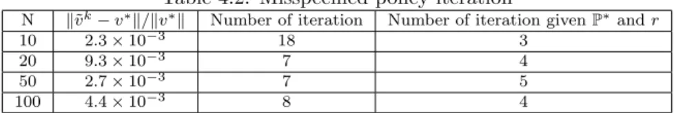
2.1 Computingx∗ and learning θ∗ (ξ∼U[−θ∗/2, θ∗/2],N = 5,W = 5) . . . . 46
3.1 Computingx∗ and learning a∗(ξ∼U[−θ∗/2, θ∗/2],N = 10) . . . . 78
Chapter 1
Introduction
Increasingly, optimization and game-theoretic problems need to be solved in uncertain and networked regimes complicated by parametric misspecification. One approach relies on estimation of these parameters through a separate learning process that necessitates aggregating data in an offline fashion. Historically, this offline avenue can be formalized by a two-step, and in effect, a serial approach: (i) The first step requires the learning of such parameters by possibly fitting a model to a set of samples, a problem that falls within the purview of statistical learning [1]; (ii) Given an estimate of such parameters, optimization algorithms can be subsequently applied. Unfortunately, in many dynamic settings complicated by streaming data and the need for online decision-making, one cannot impose such a separation in these processes and both optimization and learning need to be carried out simultaneously, particularly when exact solutions to the statistical learning problem can only be obtained in the limit. An alternate approach can be constructed in settings where an offline aggregation of data cannot be managed. Instead, in this setting, the observations are a function of the computational decisions. In this context, we consider anonlineavenue that is customized to the problem of interest (for instance stochastic Nash-Cournot games). Accordingly, in this dissertation, we consider three problem settings corrupted by misspecification in Chapters 2–4:
(i) Static stochastic convex optimization and monotone variational inequality problems; (ii) Static stochastic Nash games;
(iii) Markov decision processes.
Before proceeding, we provide a short motivation and discussion of the contributions in each of these chap-ters.
1.1
Misspecified stochastic optimization and variational
inequality problems
Convex optimization has proven to be a useful model for resolving a broad class of problems (cf. [2]). In settings where equilibria and competition assume relevance, variational inequality problems have gained im-mensely in relevance. Yet, in both contexts, it is assumed that the functions (in the context of optimization) and the maps (in the variational inequality setting) are prescribed precisely. However, as problems grow in intricacy and complexity, this assumption cannot be expected to hold. For instance, convex optimization models have found utility in portfolio optimization; however, covariance matrices in such setting rely esti-mation. Similarly, variational inequality formulations have allowed for capturing imperfectly competitive equilibrium problems; again, the parametrization of the utility functions may not always be available. In short, there is an increasing need to develop algorithms that can resolve misspecification while solving the correctly misspecified problem.
When one considers the joint problem of learning the misspecified parameter and optimizing the system, two approaches may be utilized: (i) The first of these is a sequential approach, i.e. specifying the model and/or parameters based on statistical learning and then solving the resulting optimization problems of interest. Any practically implemented sequential scheme has to terminate the learning problem after finite time. This results in an estimator of the learning problem corrupted by error and this error propagates into the solution of the optimization problem; (ii) A second approach uses the variational avenue and relies on converting the joint learning and optimization problem into a higher dimensional variational inequality problem. However, unless rather strong assumptions are imposed, the mapping associated with the varia-tional inequality problem is not necessarily monotone, which prevents us to use recently developed stochastic approximation schemes for solving monotone stochastic variational inequality problems.
Motivated by the lack of available simultaneous approaches, we propose coupled stochastic approximation schemes in Chapter 2 that allows for solving misspecified stochastic optimization and variational inequality problems. For the misspecified optimization problem, we consider the cases when the function is either strongly convex or merely convex. Almost sure convergence properties can be shown in both cases. When the function is strongly convex, the scheme displays the same optimal rate as the true parameter is available, i.e. Op1/KafterK steps. While in merely convex regimes, we can quantify the degradation associated with learning by using an averaging method, and the error in function value afterKsteps isOpln(K)/K, rather thanOp
1/Kwhen parameter information is available. To recover the original rate ofOp
1/K, we modify the averaging window and get the desired result. In addition, we consider an online counterpart
these results can be extended to a class of misspecified stochastic variational inequality problems, which are general cases for stochastic convex optimization and a range of stochastic equilibrium problems. A major difference lies in the merely monotone regimes. We need to use an iterative Tikhonov regularization to get almost-sure convergence results in that case. Also, under merely monotone assumptions, we can quantify the degradation associated with learning and show that the expected distance between the iterate and optimal set isOp
ln(K)/K.
1.2
Misspecified stochastic Nash games
While convex Nash games can be compactly captured by a variational inequality problem, the contributions of the prior section cannot adequately address the intricacies that are presented by Nash games. For instance, a key concern in the computation of equilibria is the need for developing distributed protocols that abide by privacy concerns. This motivates the next chapter of this dissertation. In particular, when designing protocols for Nash games, particularly in the absence of a centralized controller, the goal lies computing Nash equilibria when the utility functions are misspecified and rely on agent-specific information that can only be learnt through a set of offline observations. In many regimes, this set of observations may not be available. Consider, for instance, a Nash-Cournot game in which each player decides its own production level of a common commodity while the price of the commodity is based on the aggregate sales. In this regime, players may have a correct model for the price function but an incorrect estimate of its parameters. In this setting, our intent lies in developing an online scheme which relies on observing true prices that allows for learning the misspecified price function parameter. This avenue does not necessitate accumulating observations.
Motivated by these challenges, in Chapter 3, we propose schemes for computing equilibria to misspecified stochastic Nash games. In the proposed schemes, players learn the equilibrium strategy while resolving the misspecification. We consider two settings: (1) general stochastic Nash games with observable aggregate output; (2) stochastic Nash-Cournot games with unobservable aggregate output. In the first case, we propose coupled stochastic approximation distributed schemes across agents. Each agent updates its strategy through a gradient step while updating its belief regarding misspecified parameters through a learning step. Both the true equilibrium strategy and the true parameter can be shown to be achieved in an almost sure sense. The scheme displays the same optimal rate of convergence in the equilibrium strategy in a mean-squared sense as the true parameter is available. In the second case, we consider a special type of Nash games, i.e. Nash-Cournot game, and assume that the aggregate output is unavailable. In addition, we impose a
assumption for analyzing Nash-Cournot games without information of aggregate output. By using the difference between the observed true price and estimated price, we propose iterative fixed-point schemes which can learn the equilibrium strategies and the misspecified parameter simultaneously in an almost-sure sense. Furthermore, we can extend the result to nonlinear price functions.
1.3
Misspecified Markov decision processes
While the previous two sections have considered static problems, a natural extension lies in sequential decision-making problems. In particular, we consider the Markov decision-making problems (MDPs). Such problems assume relevance in a range of settings (cf. [3, 4]). Yet, in such sense, the transition matrices and the cost functions may be misspecified. Several avenues have been adopted when transition matrices are not known precisely including robust optimization and Q-learning. Yet, there is little available when cost functions are misspecified and in the presence of streaming data, traditional schemes cannot be directly employed. In fact, there is little by way of asymptotics and error analysis for resolving such MDPs with streaming data. Similarly as in misspecified stochastic optimization problems, sequential approaches can, at best, provide approximate solutions.
Motivated by these challenges, we propose a simultaneous scheme for learning and computation in Chap-ter 4 to solve a finite-state infinite horizon MDP in which the transition matrix and the parametrization of the cost function are unavailable. We consider a data-driven regime in which the learning problem is a stochastic convex optimization problem that resolves misspecification. Three types of schemes are con-sidered: (1) misspecified value iteration scheme; (2) misspecified policy iteration scheme; (3) misspecified Q-learning scheme. The misspecified value iteration scheme can be shown to converge almost surely to its true counterpart and the associated mean-squared error of convergence is provided based on the presence of learning. When the steplength is constant, we can also get an optimized error bound for the value funtion in terms of the number of iteration steps. In the context of misspecified policy iteration scheme, we can provide an analogous asymptotic almost-sure convergence statement and error analysis as in the case with information of the transition matrix and cost function. Finally, we present a constant steplength misspecified Q-learning scheme and provide a suitable error bound based on iteration steps and steplength.
1.4
Notation
Throughout the paper, we usekxk to denote the Euclidean norm of a vectorx, i.e.,kxk=√xTx. We use
matrixH is said to be a P-matrix if every principal minor of H is positive. Similarly,H is aP0-matrix if
Chapter 2
Misspecified Stochastic Optimization
and Variational Inequality Problems
2.1
Introduction
In the last two decades, robust optimization [5, 6] approaches have grown in relevance when decision-makers are faced with optimization problems with uncertain parameters. Succinctly, in such an approach, given an uncertainty set that captures the realizations assumed by such a parameter, the robustsolution represents the worst-case over this set of realizations. Naturally, an appropriate choice of such an uncertainty set is crucial and as the availability of data reaches levels hitherto unseen, there is growing interest in data-driven approaches [7] for constructing such sets. Our interest is in closely related yet distinct settings driven by data in which the point estimate of a parameter may be obtained through a learning problem, suitably defined through the aggregation of data. We provide two instances of such problems:
(i) Portfolio optimization Portfolio optimization problems prescribe the optimal constructions of port-folios over a set of assets, for which the mean and covariance of returns are not necessarily known. Traditional approaches have assumed that such returns are available while more recent robust optimization models have utilized factor-based models in constructing uncertainty sets [8, 9, 10]. An alternate, and possibly less con-servative, data-driven model of such a problem that employs a point estimate of the mean and covariance matrix requires the solution of two coupled problems: (1) A portfolio optimization problem parametrized by (θ∗,Σ∗) representing the mean and covariance matrix of returns; and (2) A learning problem that utilizes data to obtain the best (θ∗,Σ∗).
(ii) Power systems operation The operation of power grids relies on the solution of hourly (or more frequent) commitment and dispatch problems, each of which is reliant on a range of parameters that are often uncertain. These parameters include supply-side information regarding capacity of wind-power as well as load forecasts. Recently robust optimization approaches have proved to be exceedingly popular [11, 12, 13]. An alternate formulation is given by the following two coupled problems: (1) An economic dispatch problem parametrized by θ∗, a vector that captures the unknown supply and demand side parameters; and (2) A
learning problem that computesθ∗ through the accumulation of data.
We believe that such coupled formulations have broad applicability beyond merely the settings mentioned above in (i) and (ii). They may also find application in inventory control problems with stochastic demand [14, 15, 16, 17], robust network design [18], robust routing in communication networks [19], amongst others. To recap the difference between the two problem frameworks, it can be seen that (R-Opt), a robust optimization framework, minimizes the worst-case of the optimal valuef(x;θ) over the uncertainty setUθwhile (L-Opt)
considers the joint solution of an optimization problem inx, parametrized byθ∗, whereθ∗is a solution to a
learning problem with a metricg(θ). The following formulations may provide a clearer comparison:
R-Opt minimize max
θ∈Uθ f(x;θ) subject to x∈X. L-Opt minimize x∈X f(x;θ ∗) minimize θ∈Θ g(θ)
We consider regimes where the functionf(x;θ) is a convex expected-value function and the resulting problem is given by the following:
min
x∈X E[f(x;θ
∗, ξ(ω))], (Po
x(θ∗))
whereX⊆Rnis a closed and convex set,ξ: Ω→Rdis ad−dimensional random variable defined on a
prob-ability space (Ω,Fx,Px),f :X×Rd×Rm→Ris a real-valued function, andθ∗ denotes anm−dimensional
vector of parameters. Estimating such parameters often requires the resolution of a suitably defined learning problem, given by a stochastic optimization problem (Lθ), and defined next:
min
θ∈Θ g(θ),E[g(θ;η)], (Lθ)
where Θ⊆Rm is a closed and convex set, η : Λ→Rp is a random variable defined on a probability space
(Λ,Fθ,Pθ), andg: Θ×Λ→Ris a real-valued function. When one considers the joint problem of learning
and optimization, then there are at least two obvious approaches that immediately emerge as possibilities: (a) Sequential approach: Consider an inherently serial process wherein the first stage incorporates a model/parameter specification phase based on statistical learning while the second stage leverages these findings in developing and solving the actual optimization problem of interest. Such an ordering relies on the learning problems being relatively small and tractable compared to the optimization problems, ensuring that accurate solutions are available within a reasonable time period. Strictly speaking, if one terminates the learning process prematurely with an estimator ˆθ, the resulting estimator is essentially corrupted by
error in that ˆθ 6=θ∗. This error propagates into the solution ˆxof the computational problem, denoted by Po
x(ˆθ) and the associated gap might be quite significant. Note that unless the learning problem is solvable
via a finite termination algorithm, such a approach cannot provide asymptotic statements but can, at best, provide approximate solutions. Consequently, an inherently serial process reliant on a prematurely truncated learning scheme often fails to provide accurate solutions to the computational problem.
(b) Variational approach: Under suitable convexity and differentiability requirements, the following holds:
x∗ solves (Pxo(θ∗)) andθ∗ solves (Lθ),
if and only if (x∗, θ∗) is a solution to the (stochastic) variational inequality problem VI(Z, F) [20] where
Z ,X×Θ andH(z), E[∇xf(x;θ, ξ)] E[∇θg(θ;η)] .
Recall thatz∗is a solution to VI(Z, F) if (z−z∗)TF(z)≥0 for allz∈Z. Furthermore, ifx∗ andθ∗ denote
solutions to (Po
x(θ∗)) and (Lθ), respectively, then an oft-used avenue in obtaining a solution (x∗, θ∗) entails
obtaining a solution to VI(Z, F). However, unless rather strong assumptions are imposed, the mapH is not necessarily monotone, precluding the use of recently developed stochastic approximation schemes for solving monotone stochastic variational inequality problems [21, 22, 23], extragradient-based variants [24, 25], and accelerated approaches [26].
Simultaneous approach: This chapter is motivated by the inadequacy of available approaches and, more generally, the absence ofasymptotically convergent schemes with provable non-asymptotic rates. We present a framework where the learning and the computational problems are solvedsimultaneouslyvia a joint set of stochastic approximation schemes. Such an avenue has several advantages. First, under such an approach, one can provide rigorous statements of asymptotic convergence of the obtained estimators for both, the solution to the computational problem and the associated learning problem. Second, error bounds on the expected error can be provided for a fixed number of steps under a regime with constant and diminishing steplengths. Third, the statements may be extended to the variational regime in which the computational problem is given by the variational counterpart of (Po
x(θ∗)), given by (Pxv(θ∗)); such a problem requires an
x∗∈X such that
E[F(x∗;θ∗, ξ(ω))]T(x−x∗) ≥ 0, ∀x ∈ X, (Pxv(θ∗))
probability space (Ω,Fx,Px),F:X×Rd×Rm→Rn is a real-valued continuous mapping. Note that when
F(x∗;θ∗, ξ) , ∇xf(x∗;θ∗, ξ), this reduces to a convex optimization problem. Furthermore, the choice of
using a variational problem, rather than merely an optimization problem, is founded on the need to model a variety of multiagent settings complicated by a breadth of strategic interactions, ranging from purely cooperative to distinctly noncooperative [27].
2.1.1
Related decision-making models
While unaware of the availability of general purpose tools that can resolve precisely such problems, we describe settings where such questions have assumed relevance:
Adaptive control [28]: In tracking problems in adaptive control [29], the authors consider a perturbation approach for analyzing a adaptive tracking algorithm and consider three estimation schemes, specifically least mean squares (LMS) scheme, its recursive variant (RLMS), and the Kalman filter (which requires some distributional assumptions on the noise). First, much of this treatment is in the unconstrained regime with tractable (often quadratic estimation objectives), allowing for deriving closed-form (and often linear) update rules. Second, when the noise in the estimation process is Gaussian, the Kalman filter provides a minimum variance estimator. If on the other hand, the noise is non-Gaussian, then the Kalman filter provides the optimal linear estimator (in the sense that no linear filter provides smaller variance). In fact, these assumptions often form the basis of most adaptive control algorithms (cf. [30] and [31] for a discussion adaptive control and stochastic approximation.) Our focus is on static stochastic problems with far less assumptions on the nature of the problem and the associated distributions. Specifically, we allow for more general stochastic convex objectives (or monotone maps in the context of VIs) in either the optimization or the learning problem, allow for convex feasibility sets for both the optimization or the learning problems, and impose relatively mild moment assumptions on the noise (unlike the Gaussian assumptions that are necessary in some of the estimation models).
Iterative learning control: A related avenue lies in iterative learning control (ILC) has its roots in the studies by Uchiyama [32] and Arimoto et al. [33]. ILC [34] is a form of tracking control employed for repetitive control problems, instances being chemical batch processes, robot arm manipulators, and reliability testing rigs. Our problem is more restrictive in its focus (static problems) but allow for more general settings in terms of nonlinearity and the underlying distributional requirements.
Multi-armed bandit problems: The multi-armed bandit (MAB) problem considers the question of how to play given a collection of slot machines faced by a gambler. Each machine provides a random reward from a distribution specific to that machine. The gambler aims to maximize the expected sum of rewards
earned through a sequence of lever pulls. The total discounted reward is maximized by the index policy that pulls the bandit having greatest value of the Gittins index [35]. In effect, the reward function needs to be learnt while optimizing the system. There has been significant research on such problems over the last several decades, including on the question of computation [36] and finite-time analysis [37].
Finally, related questions have also been studied in revenue management where [38] examined the devas-tating effect of learning with an incorrect model while maximizing revenue.
2.1.2
Outline and contributions
Broadly speaking, this chapter focuses on the development of stochastic approximation schemesthat gen-erate itgen-erates {xk} and {θk} and makes the following contributions. (i) In Section 2.2, we prove the a.s.
convergence of the produced iterates to the prescribed solutions and derive error bounds in a standard and an averaging regime. In particular, we quantify the degradation in the convergence rate from introducing an additional learning phase; (ii) Section 2.2 concludes with a precise non-asymptotic bound on the average regret associated with employing the proposed scheme instead of an offline algorithm; (iii) In Section 2.3, we extend the a.s. convergence results to accommodate stochastic variational inequality problems, rather than merely convex optimization problems. Error analysis is carried out under a suitably defined growth property; (iv) In Section 2.4, we provide some supporting numerics and conclude in Section 2.5.
2.2
Stochastic optimization problems with imperfect information
In this section, we focus on examining (Po
x(θ∗)) under various assumptions. We begin by stating the coupled
stochastic approximation scheme and providing the necessary assumptions in Section 2.2.1. Convergence analysis of the presented scheme is provided in Section 2.2.2 while diminishing and constant steplength rate analysis is performed in Section 2.2.3. We conclude with a discussion of an online algorithm with the associated bounds on the decay of average regret in Section 2.2.4.
2.2.1
Algorithm statement and assumptions
As mentioned in the previous section, we propose a set of coupled stochastic approximation schemes for computingx∗ andθ∗.
Algorithm 1 (Coupled SA schemes for stochastic optimization problems). Step 0. Given x0 ∈ X, θ0∈Θand sequences{γk,x, γk,θ},k:= 0 Step 1. xk+1:= ΠX xk−γk,x(∇xf(xk;θk) +wk), k≥0 (Optk) θk+1:= Π Θ θk−γk,θ(∇θg(θk) +vk), k≥0 (Learnk) where wk ,∇xf(xk;θk, ξk)− ∇xf(xk;θk) andvk ,∇θg(θk;ηk)− ∇θg(θk).
Step 2. If k > K, stop; elsek:=k+ 1, go to Step. 1.
We begin by stating an assumption on the functions f andg.
Assumption 1 (Problem properties, A1-1). Suppose the following hold:
(i) For every θ ∈Θ, f(x;θ) is strongly convex and continuously differentiable with Lipschitz continuous gradients in xwith convexity constantµxand Lipschitz constant Lx, respectively.
(ii) For everyx∈X, the gradient ∇xf(x;θ)is Lipschitz continuous in θ with constantLθ.
(iii) The functiong(θ)is strongly convex and continuously differentiable with Lipschitz continuous gradients in θwith convexity constantµθ and Lipschitz constantCθ, respectively.
Under Assumption (A1-1), the coupled problem admits a unique solution, as shown next. Lemma 1 (Solvability). Consider the problems (Po
x(θ∗)) and (Lθ) and suppose assumption (A1) holds.
Then(Po
x(θ∗))and(Lθ)collectively admit a unique solution.
Proof. This follows from the strong convexity ofg over Θ and the strong convexity off(•;θ) overX. Additionally, we make the following assumptions on the steplength sequences employed in the algorithm. Assumption 2 (Steplength requirements, A2-1). Let {γk,x} and{γk,θ} be chosen such that:
(i) P∞k=0γk,x=∞,P∞k=0γk,x2 <∞
(ii) γk,θ=γk,xL2θ/(µxµθ).
We define a new probability space (Z,F,P), whereZ ,Ω×Λ,F ,Fx× Fθ andP,Px×Pθ. We use
Fk to denote the sigma-field generated by the initial points (x0, θ0) and errors (wl, vl) forl= 0,1,· · ·, k−1,
i.e., F0 =
(x0, θ0) and F
k =
Assumption 3 (A3). Let the following hold:
(i) E[wk| Fk] = 0andE[vk | Fk] = 0a.s. for allk.
(ii) E[kwkk2| Fk]≤νx2 andE[kvkk2| Fk]≤ν2θ a.s.for allk.
We conclude this subsection by stating three results (without proof) that will be subsequently employed in developing our convergence statements. The first two of these are relatively well-known super-martingale convergence results (cf. [39, Lemma 10, Pg. 49–50])
Lemma 2. Let vk be a sequence of nonnegative random variables adapted toσ-algebraFk and such that
E[vk+1|Fk]≤(1−uk)vk+βk for allk≥0 almost surely,
where0≤uk ≤1,βk ≥0, andP∞k=0uk =∞,P∞k=0βk<∞andlimk→∞ukβk = 0. Then,vk →0 a.s.
Lemma 3. Let vk,uk,βk andγk be non-negative random variables adapted toσ-algebraFk. IfP∞k=0uk<
∞,P∞k=0βk <∞ and
E[vk+1|Fk]≤(1 +uk)vk−γk+βk for allk≥0 almost surely.
Then, {vk}is convergent andP∞k=0γk<∞almost surely.
Finally, we present a contraction result reliant on monotonicity and Lipschitz continuity requirements (cf. [40, Theorem 12.1.2, Pg. 1109]).
Lemma 4. LetH :K→Rn be a mapping that is strongly monotone over K with constantµ, and Lipschitz
continuous overK with constantL. Ifq,p1−2µγ+γ2L2, then for anyγ >0, we have that for anyx, y, we have kΠK(x−γH(x))−ΠK(y−γH(y))k ≤qkx−yk.
2.2.2
Almost-sure convergence
Our first convergence result shows that under the prescribed assumptions, Algorithm 1 generates a sequence of iterates that converges to the unique solution.
Proposition 1 (Almost-sure convergence under strong convexity of f). Suppose (A1-1), (A2-1) and (A3) hold. Let {xk, θk} be computed via Algorithm 1. Then, xk → x∗ and θk → θ∗ a.s. as k → ∞, where θ∗ denotes the unique solution of (L
Proof. Note thatx∗ = ΠX(x∗−γk,x∇xf(x∗;θ∗)).Then, by the nonexpansivity of the Euclidean projector,
kxk+1−x∗k2may be bounded as follows:
kxk+1−x∗k2=kΠ
X(xk−γk,x(∇xf(xk;θk) +wk))−ΠX(x∗−γk,x∇xf(x∗;θ∗))k2
≤ k(xk−x∗)−γk,x(∇xf(xk;θk)− ∇xf(x∗;θ∗))−γk,xwkk2.
By adding and subtractingγk,x∇xf(x∗, θk), this expression can be further expanded as follows:
k(xk−x∗)−γ
k,x(∇xf(xk;θk)− ∇xf(x∗;θk))−γk,x(∇xf(x∗;θk)− ∇xf(x∗;θ∗))−γk,xwkk2
=k(xk−x∗)−γk,x(∇xf(xk;θk)− ∇xf(x∗;θk))k2+γk,x2 k∇xf(x∗;θk)− ∇xf(x∗;θ∗)k2+γk,x2 kwkk2
−2γk,x[(xk−x∗)−γk,x(∇xf(xk;θk)− ∇xf(x∗;θk))]T(∇xf(x∗;θk)− ∇xf(x∗;θ∗))
−2γk,x[(xk−x∗)−γk,x(∇xf(xk;θk)− ∇xf(x∗;θk))]Twk+ 2γk,x2 (∇xf(x∗;θk)− ∇xf(x∗;θ∗))Twk.
By leveraging the fact thatE[wk| Fk] = 0, we have
E[kxk+1−x∗k2| Fk]≤Term 1+Term 2+Term 3+γ2k,xE[kwkk2| Fk], (2.1)
whereTerms 1 – 3are defined as follows:
Term 1,k(xk−x∗)−γk,x(∇xf(xk;θk)− ∇xf(x∗;θk))k2,
Term 2,γ2k,xk∇xf(x∗;θk)− ∇xf(x∗;θ∗)k2,
andTerm 3,−2γk,x[(xk−x∗)−γk,x(∇xf(xk;θk)− ∇xf(x∗;θk))]T(∇xf(x∗;θk)− ∇xf(x∗;θ∗)).
By Lemma 4 and (A1-1), it follows that
Term 1≤(1−2γk,xµx+γk,x2 L2x)kxk−x∗k2. (2.2)
Furthermore, the Lipschitz continuity of∇xf(x∗;θ) inθ (A1-1) allows for deriving the following bound:
Term 2≤γk,x2 L2θkθk−θ∗k2. (2.3)
triangle inequality, we obtain 2γk,xk(xk−x∗)−γk,x(∇xf(xk;θk)− ∇xf(x∗;θk))kk∇xf(x∗;θk)− ∇xf(x∗;θ∗)k ≤2γk,x q 1−2γk,xµx+γ2k,xL2xkxk−x∗kLθkθk−θ∗k ≤2γk,xLθkxk−x∗kkθk−θ∗k ≤γk,xµxkxk−x∗k2+γk,x(L2θ/µx)kθk−θ∗k2, (2.4)
where the last inequality follows from 2aTb≤ kak2+kbk2.Combining (2.1), (2.2), (2.3) and (2.4), we get
E[kxk+1−x∗k2| Fk]≤(1−γk,xµx+γk,x2 L2x)kxk−x∗k2
+ (γk,xL2θ/µx+γk,x2 L2θ)kθk−θ∗k2+γk,x2 νx2.
(2.5)
Recall that θ∗ satisfies the fixed point relationship θ∗ = Π
Θ(θ∗−γθ,k∇θg(θ∗)), which, together with
non-expansivity of the Euclidean projector, allows for deriving the following bound onkθk+1−θ∗k2:
kθk+1−θ∗k2=kΠΘ(θk−γθ,k(∇θg(θk) +vk))−ΠΘ(θ∗−γθ,k∇θg(θ∗))k2
≤ kθk−θ∗−γθ,k(∇θg(θk)− ∇θg(θ∗))−γθ,kvkk2
=kθk−θ∗−γ
θ,k(∇θg(θk)− ∇θg(θ∗))k2+γθ,k2 kvkk2−2(θk−θ∗−γθ,k(∇θg(θk)− ∇θg(θ∗)))Tvk.
By taking conditional expectations and by recalling thatE[vk | Fk] = 0, we obtain the following bound:
E[kθk+1−θ∗k2| Fk]≤ kθk−θ∗−γk,θ(∇θg(θk)− ∇θg(θ∗))k2+γk,θ2 E[kvkk2| Fk]
≤qk,θ2 kθk−θ∗k2+γk,θ2 νθ2,
(2.6)
whereqk,θ,
q
1−2γk,θµθ+γk,θ2 Cθ2. Next, by adding (2.5) and (2.6) and by invoking (A2-1), we obtain the
following bound. E[kxk+1−x∗k2| Fk] +E[kθk+1−θ∗k2| Fk] ≤(1−γk,xµx+γk,x2 L2x)kxk−x∗k2+ (qk,θ2 +γk,xL2θ/µx+γk,x2 L2θ)kθk−θ∗k2+γk,x2 νx2+γk,θ2 νθ2 = (1−γk,xµx+γk,x2 L2x)kxk−x∗k2+ (1−γk,xL2θ/µx+γk,x2 (L2θ+L4θCθ2/(µ2xµ2θ)))kθk−θ∗k2 +γk,x2 νx2+γ2k,xνθ2L4θ/(µ2xµ2θ) ≤(1−αγk,x+βγ2k,x)(kxk−x∗k2+kθk−θ∗k2) +δγk,x2 ,
whereα= min{µx, L2θ/µx},β = max{L2x, L2θ+L4θCθ2/(µ2xµ2θ)} andδ=νx2+νθ2L4θ/(µ2xµ2θ). From (A2-1), we
have thatP∞k=0(αγk,x−βγk,x2 ) =∞, P∞k=0δγk,x2 <∞,and
lim
k→∞
δγ2
k,x
αγk,x−βγk,x2 = 0.
Then, by invoking the super-martingale convergence theorem (Lemma 2), we have thatkxk−x∗k2+kθk−
θ∗k2→0a.s.as k→ ∞, which implies thatxk→x∗ andθk →θ∗ a.s.as k→ ∞.
Next we weaken the strong convexity requirement on the functionf through the following assumption. Assumption 4 (A1-2). Suppose the following holds in addition to (A1-1 (ii)) and (A1-1 (iii)).
(i) For everyθ∈Θ,f(x;θ)is convex and continuously differentiable with Lipschitz continuous gradients in xwith Lipschitz constantLx.
Furthermore, we make the following assumptions on the steplength sequences employed in the algorithm. Assumption 5 (A2-2). Let{γk,x},{γk,θ} and some constantτ ∈(0,1)be chosen such that:
(i) P∞k=0γk,x2−τ <∞ andP∞k=0γ2 k,θ<∞, (iii) P∞k=0γk,x=∞ andP∞k=0γk,θ=∞, (iii) βk= γτ k,x 2γk,θµθ ↓0 ask→ ∞.
Proceeding as in the previous result, we present a convergence result under these weakened conditions.
Theorem 1 (Almost-sure convergence under convexity of f). Suppose (A1-2), (A2-2) and (A3) hold. SupposeX is bounded and the solution setX∗ of (Po
x(θ∗))is nonempty. Let{xk, θk} be computed via
Algorithm 1. Then, θk →θ∗ a.s. as k → ∞, and xk converges to a random point in X∗ a.s. as k→ ∞, where θ∗ denotes the unique solution of (L
θ)andX∗ denotes the solution set of (Pxo(θ∗)).
Proof. By the nonexpansivity of the Euclidean projector, we have for anyx∗∈X∗ that
kxk+1−x∗k2=kΠX(xk−γk,x(∇xf(xk;θk) +wk))−ΠX(x∗)k2
By adding and subtractingγk,x∇xf(x∗, θk), this expression can be further expanded as follows:
k(xk−x∗)−γk,x∇xf(xk;θ∗)−γk,x(∇xf(xk;θk)− ∇xf(xk;θ∗))−γk,xwkk2
=k(xk−x∗)−γk,x∇xf(xk;θ∗)k2+γk,x2 k∇xf(xk;θk)− ∇xf(xk;θ∗)k2+γk,x2 kwkk2
−2γk,x[(xk−x∗)−γk,x∇xf(xk;θ∗)]T(∇xf(xk;θk)− ∇xf(xk;θ∗))
−2γk,x[(xk−x∗)−γk,x∇xf(xk;θ∗)]Twk+ 2γk,x2 (∇xf(xk;θk)− ∇xf(xk;θ∗))Twk.
Noting thatE[wk| Fk] = 0, we have
E[kxk+1−x∗k2| Fk]≤Term 1+Term 2+Term 3+γ2k,xE[kwkk2| Fk], (2.7)
whereTerms 1 – 3are defined as follows:
Term 1,k(xk−x∗)−γk,x∇xf(xk;θ∗)k2,
Term 2,γk,x2 k∇xf(xk;θk)− ∇xf(xk;θ∗)k2,
andTerm 3,−2γk,x[(xk−x∗)−γk,x∇xf(xk;θ∗)]T(∇xf(xk;θk)− ∇xf(xk;θ∗)).
By invoking the convexity off(x;θ) inxand the gradient inequality (see A1-2), we have that
Term 1=kxk−x∗k2+γ2k,xk∇xf(xk;θ∗)k2−2γk,x(xk−x∗)T∇xf(xk;θ∗)
≤ kxk−x∗k2+γ2k,xk∇xf(xk;θ∗)k2−2γk,x(f(xk;θ∗)−f(x∗;θ∗))
≤ kxk−x∗k2+ 2γk,x2 k∇xf(xk;θ∗)− ∇xf(x∗;θ∗)k2+ 2γk,x2 k∇xf(x∗;θ∗)k2
−2γk,x(f(xk;θ∗)−f(x∗;θ∗)),
where the last inequality follows from the identityk(a−b) +bk2 ≤2ka−bk2+ 2kbk2. From the Lipschitz
continuity of∇xf(x;θ) inx, the right hand side can be bounded as follows:
kxk−x∗k2+ 2γk,x2 k∇xf(xk;θ∗)− ∇xf(x∗;θ∗)k2+ 2γk,x2 k∇xf(x∗;θ∗)k2−2γk,x(f(xk;θ∗)−f(x∗;θ∗))
≤(1 + 2γk,x2 L2x)kxk−x∗k2+ 2γk,x2 k∇xf(x∗;θ∗)k2−2γk,x(f(xk;θ∗)−f(x∗;θ∗)). (2.8)
By the Lipschitz continuity of∇xf(x;θ) inθ (A1-2),
By adding and subtracting∇xf(x∗;θ∗), and by invoking the Lipschitz continuity of ∇xf(x;θ) inx(A1-2)
and the triangle inequality, we may derive a bound forTerm 3as follows:
Term 3≤2γk,xk(xk−x∗)−γk,x∇xf(xk;θ∗)kk∇xf(xk;θk)− ∇xf(xk;θ∗)k
≤2γk,xk(xk−x∗)−γk,x(∇xf(xk;θ∗)− ∇xf(x∗;θ∗))−γk,x∇xf(x∗;θ∗)kLθkθk−θ∗k
≤2γk,x (1 +γk,xLx)kxk−x∗k+γk,xk∇xf(x∗;θ∗)kLθkθk−θ∗k
= 2γk,xLθkxk−x∗kkθk−θ∗k+ 2γk,x2 LθLxkxk−x∗kkθk−θ∗k+ 2γk,x2 Lθk∇xf(x∗;θ∗)kkθk−θ∗k.
By using the fact that 2ab≤a2+b2, we have further that
Term 3≤γk,x2−τL2θkxk−x∗k2+γk,xτ kθk−θ∗k2+γk,x2 LθLxkxk−x∗k2
+γk,x2 LθLxkθk−θ∗k2+γk,x2 L2θkθk−θ∗k2+γ2k,xk∇xf(x∗;θ∗)k2,
(2.10)
whereτ∈(0,1) is chosen to satisfy (A2-2). Combining (2.7), (2.8), (2.9) and (2.10), we obtain the following bound on the conditional error.
E[kxk+1−x∗k2| Fk]≤(1 +γk,x2−τL
2
θ+γk,x2 (2L2x+LθLx))kxk−x∗k2+ (γk,xτ +γk,x2 (2L2θ+LθLx))kθk−θ∗k2
+ 3γ2k,xk∇xf(x∗;θ∗)k2−2γk,x(f(xk;θ∗)−f(x∗;θ∗)). (2.11)
From (2.6), we have that
E[kθk+1−θ∗k2| Fk]≤q2k,θkθk−θ∗k2+γk,θ2 νθ2, (2.12) whereqk,θ, q 1−2γk,θµθ+γk,θ2 Cθ2. Choose βk = γτ k,x
2γk,θµθ by (A2-2). Note that by assumptionβk+1≤βk.
By multiplying the left hand side of (2.12) byβk+1and adding to the left hand side of (2.11), we get
E[kxk+1−x∗k2| Fk] +βk+1E[kθk+1−θ∗k2| Fk]≤E[kxk+1−x∗k2| Fk] +βkE[kθk+1−θ∗k2| Fk] (2.13) ≤(1 +γk,x2−τL2θ+γk,x2 (2L2x+LθLx))kxk−x∗k2+ (βkq2k,θ+γk,xτ +γk,x2 (2L2θ+LθLx))kθk−θ∗k2 + 3γk,x2 k∇xf(x∗;θ∗)k2+βkγk,θ2 νθ2−2γk,x(f(xk;θ∗)−f(x∗;θ∗)) ≤(1 +γk,x2−τL2θ+γk,x2 (2L2x+LθLx))kxk−x∗k2+ βkq2k,θ+γk,xτ +γk,x2 (2L2θ+LθLx) βk | {z } Term 4 ·βkkθk−θ∗k2 + 3γk,x2 k∇xf(x∗;θ∗)k2+βkγk,θ2 νθ2−2γk,x(f(xk;θ∗)−f(x∗;θ∗)).
Term 4 on the right hand side of (2.13) can be further expanded as βkq2k,θ+γτk,x+γk,x2 (2L2θ+LθLx) βk =qk,θ2 + γτ k,x+γ2k,x(2L2θ+LθLx) βk = 1−2γk,θµθ+γk,θ2 Cθ2+ γτ k,x βk + γ2 k,x(2L2θ+LθLx) βk = 1 +γk,θ2 Cθ2+ 2γk,θγk,x2−τµθ(2L2θ+LθLx). (2.14)
Combining (2.13) and (2.14), we get
E[kxk+1−x∗k2| Fk] +βk+1E[kθk+1−θ∗k2| Fk] ≤(1 +γk,x2−τL2 θ+γk,x2 (2L2x+LθLx))kxk−x∗k2+ (1 +γ2k,θCθ2+ 2γk,θγk,x2−τµθ(2L2θ+LθLx))βkkθk−θ∗k2 + 3γk,x2 k∇xf(x∗;θ∗)k2+βkγk,θ2 νθ2−2γk,x(f(xk;θ∗)−f(x∗;θ∗)) ≤(1 +γk,θ2 Cθ2+ 2γk,θγk,x2−τµθ(2L2θ+LθLx))(kxk−x∗k2+βkkθk−θ∗k2) + (γk,x2−τL2 θ+γk,x2 (2L2x+LθLx))kxk−x∗k2 + 3γk,x2 k∇xf(x∗;θ∗)k2+βkγk,θ2 νθ2−2γk,x(f(xk;θ∗)−f(x∗;θ∗)).
We define the following:
uk ,γk,θ2 Cθ2+ 2γk,θγk,x2−τµθ(2L2θ+LθLx), σk ,2γk,x(f(xk;θ∗)−f(x∗;θ∗)),
andρk ,(γk,x2−τL2θ+γ2k,x(2L2x+LθLx))kxk−x∗k2+ 3γk,x2 k∇xf(x∗;θ∗)k2+βkγk,θ2 νθ2.
Then, we have
E[kxk+1−x∗k2| Fk] +βk+1E[kθk+1−θ∗k2| Fk]≤(1 +uk)(kxk−x∗k2+βkkθk−θ∗k2) +ρk−σk.
By boundedness ofX and (A2-2), we have thatP∞k=0uk<∞andP∞k=0ρk <∞. So, by Lemma 3 we get
that there exists a random variableV such thatkxk−x∗k2+β
kkθk−θ∗k2→V in an almost sure sense as
k→ ∞andP∞
k=0σk=P∞k=02γk,x(f(xk;θ∗)−f(x∗;θ∗))<∞.
By (A2-2), Lemma 2 and (2.12), we can get that kθk−θ∗k →0 a.s. as k → ∞. Thus, it follows that
kxk−x∗k →V a.s.ask→ ∞. SinceP∞
k=0γk,x=∞, we get lim infk→∞f(xk;θ∗) =f(x∗;θ∗)a.s.ask→ ∞.
Since the setX is closed, all accumulation points of{xk}lie inX. Furthermore, sincef(xk;θ∗)→f(x∗;θ∗)
along a subsequencea.s., by continuity off it follows that{xk} has a subsequence converginga.s.to some
sincekxk−x∗kis convergent for anyx∗∈X∗ a.s., the entire sequence{xk}converges to some random point
inX∗ a.s.
2.2.3
Diminishing and constant steplength rate analysis
While the previous section focused on the almost sure convergence of the prescribed learning and computa-tional schemes, a natural question is whether one can develop rate statements. We begin with an examination of the global rate of convergence and show thatO(1/K) rate estimate is derived for an upper bound on the mean-squared error in the solutionxK whenf(•;θ∗) is strongly convex in (•) andK represents the number
of steps, consistent with the result obtained for stochastic approximation (cf. [41, 42]). In addition, it is seen that when the function loses strong convexity, an analogous rate estimate is available by using averaging, akin to an approach first employed in [43], where longer stepsizes were suggested with consequent averaging of the obtained iterates.
Proposition 2 (Rate estimates for strongly convex f). Suppose (A1-1) and (A3) hold. Suppose
γx,k =λx/k and γθ,k = λθ/k with λx > 1/µx and λθ > 1/(2µθ). Let E[k∇xf(xk;θk) +wkk2]≤ M2 and
E[k∇θg(θk) +vkk2]≤Mθ2 for allxk∈X andθk∈Θ. Let{xk, θk} be computed via Algorithm 1. Then, the
following hold after K iterations:
E[kθK−θ∗k2]≤ Qθ(λθ) K andE[kx K−x∗k2]≤Qx(λx) K , whereQθ(λθ),maxλ2θMθ2(2µθλθ−1)−1,E[kθ1−θ∗k2] , Qx(λx),max n λ2xMf2(µxλx−1)−1,E[kx1−x∗k2] o , andMf, s M2+L 2 θQθ(λθ) µxλx .
Proof. SupposeAk , 12kxk−x∗k2 andak ,E[Ak]. Then, Ak+1 may be bounded as follows by using the
non-expansivity of the Euclidean projector:
Ak+1= 1 2kx k+1−x∗k2=1 2 ΠX xk−γx,k(∇xf(xk;θk) +wk)−ΠX(x∗) 2 ≤ 1 2kx k−x∗−γ x,k(∇xf(xk;θk) +wk)k2 =Ak+ 1 2γ 2 x,kk∇xf(xk;θk) +wkk2−γx,k(xk−x∗)T(∇xf(xk;θk) +wk). (2.15)
Note thatE[(xk−x∗)Twk] =E[E[(xk−x∗)Twk|Fk]] =E[(xk−x∗)TE[wk|Fk]] = 0. By taking expectations on
both sides of (2.15) and by invoking the boundsE[k∇xf(xk;θk)+wkk2]≤M2andE[k∇θg(θk)+vkk2]≤Mθ2,
it follows that ak+1≤ak+ 1 2γ 2 x,kM2−γx,kE[(xk−x∗)T∇xf(xk;θk)]. (2.16)
Butf(x;θ) is strongly convex inxwith constantµxfor every θ∈Θ, leading to the following expression:
E[(xk−x∗)T∇xf(xk;θk)] =E[(xk−x∗)T(∇xf(xk;θk)− ∇xf(x∗;θk))]
+E[(xk−x∗)T(∇xf(x∗;θk)− ∇xf(x∗;θ∗))] +E[(xk−x∗)T∇xf(x∗;θ∗)]
≥µxE[kxk−x∗k2] +E[(xk−x∗)T(∇xf(x∗;θk)− ∇xf(x∗;θ∗))].
(2.17)
Combining (2.16) and (2.17), we get
ak+1≤(1−2γx,kµx)ak+ 1 2γ 2 x,kM2−γx,kE[(xk−x∗)T(∇xf(x∗;θk)− ∇xf(x∗;θ∗))] ≤(1−2γx,kµx)ak+ 1 2γ 2 x,kM2+ 1 2γx,kµxE[kx k−x∗k2] +1 2 γx,k µx E[k∇xf(x ∗;θk)− ∇ xf(x∗;θ∗)k2] ≤(1−γx,kµx)ak+ 1 2γ 2 x,kM2+ 1 2 γx,k µx L 2 θE[kθk−θ∗k2]. (2.18)
Supposeγθ,k =λθ/k. Since the functiong(θ) is strongly convex, we can use the standard rate estimate (cf.
inequality (5.292) in [42]) to get the following
E[kθk−θ∗k2]≤ Qθ(λθ)
k , (2.19)
whereQθ(λθ),maxλθ2Mθ2(2µθλθ−1)−1,E[kθ1−θ∗k2] withλθ>1/(2µθ). Supposeγx,k=λx/k,
allow-ing us to claim the followallow-ing:
ak+1≤ 1−µxλx k ak+ 1 2 λ2 xM2 k2 + 1 2 λxL2θQθ(λθ) µxk2 = 1−µxλx k ak+ 1 2 λ2 xMf2 k2 , whereMf, q M2+L2θQθ(λθ)
µxλx . By assuming thatλx>1/µx, the result follows by observing that
E[kxk−x∗k2]≤ Qx(λx) k , whereQx(λx),max n λ2 xMf2(µxλx−1)−1,E[kx1−x∗k2] o .
Remark: Notice that here we assume that f andg are both smooth and strongly convex. A more general framework is that of composite objectives where the objective is a sume of nonsmooth and smooth stochastic components. Lan [44] proposed the accelerated stochastic approximation (AC-SA) algorithm for solving stochastic composite optimization (SCO) problems and proved that it achieves the optimal rate. In related work, Ghadimi and Lan [45, 46] propose a multi-stage AC-SA algorithm, which possesses an optimal rate of convergence for solving strongly convex SCO problems in terms of the dependence on different problem parameters. While this problem class is beyond the current scope, this approach may aid in refinement of the constants in the Proposition 2 in some regimes.
A shortcoming of the previous result is the need for strong convexity of f(x, θ) in xfor everyθ∈Θ. In our next result, we weaken this requirement and allow for a merely convexf, extending the optimal constant stepsize result in [42]. Specifically, given a prescribed number of iterations, say K, the optimal “constant stepsize” derives the error minimizing steplength; in other words,γk =γ for 1≤k≤K. This is in contrast
with the constant stepsize result presented in Proposition 3, where γk =γ for all k. steps. The following
Lipschitzian assumption is imposed on the functionf(x;θ).
Assumption 6 (A6). Suppose the following holds in addition to (A1-2). (i) For every x∈X,f(x;θ) is Lipschitz continuous inθ with constantDθ.
Theorem 2 (Rate estimates under convexity of f). Suppose (A3) and (A6) hold. Suppose E[kxk− x∗k2] ≤ M2
x, E[k∇xf(xk;θk) +wkk2] ≤M2 and E[k∇θg(θk) +vkk2] ≤ Mθ2 for all xk ∈ X and θk ∈ Θ.
Let {xk, θk} be computed via Algorithm 1. For 1≤i, t≤k, we definev
t, Pkγx,t s=iγx,s
,x˜i,k ,Pkt=ivtxt and
DX,maxx∈Xkx−x1k. Suppose for1≤t≤K,γx is defined as follows:
γx= s 4D2 X+L2θQθ(λθ)(1 + lnK) (M2+M2 x)K , where Qθ(λθ),max λ2
θMθ2(2µθλθ−1)−1,E[kθ1−θ∗k2] , and γθ,k =λθ/K with λθ >1/(2µθ). Then the
following holds for 1≤i≤K:
E[f(˜xi,K;θK)−f(x∗;θ∗)]≤ p Qθ(λθ)Dθ+Ci,K √ BK √ K ,
Proof. By using the same notation in Proposition 2, we have from (2.16) that ak+1≤ak+ 1 2γ 2 x,kM2−γx,kE[(xk−x∗)T∇xf(xk;θk)] ≤ak+1 2γ 2 x,kM2−γx,kE[(xk−x∗)T∇xf(xk;θ∗)]−γx,kE[(xk−x∗)T(∇xf(xk;θk)− ∇xf(xk;θ∗))]. (2.20) Note thatf(x;θ) is convex inxfor everyθ∈Θ, allowing us to leverage the gradient inequality.
E[(xk−x∗)T∇xf(xk;θ∗)]≥E[f(xk;θ∗)−f(x∗;θ∗)]. (2.21)
Combining (2.20) and (2.21), we obtain the following:
ak+1≤ak+
1 2γ
2
x,kM2−γx,kE[f(xk;θ∗)−f(x∗;θ∗)]−γx,kE[(xk−x∗)T(∇xf(xk;θk)− ∇xf(xk;θ∗))].
This allows for constructing the following bounds:
γx,kE[f(xk;θ∗)−f(x∗;θ∗)] ≤ak−ak+1+ 1 2γ 2 x,kM2−γx,kE[(xk−x∗)T(∇xf(xk;θk)− ∇xf(xk;θ∗))] ≤ak−ak+1+ 1 2γ 2 x,kM2+ 1 2γ 2 x,kE[kxk−x∗k2] + 1 2E[k∇xf(x k;θk)− ∇ xf(xk;θ∗)k2] ≤ak−ak+1+1 2γ 2 x,kM2+ 1 2γ 2 x,kMx2+ 1 2L 2 θE[kθk−θ∗k2] ≤ak−ak+1+ 1 2γ 2 x,k(M2+Mx2) + 1 2 L2 θQθ(λθ) k , (2.22)
where the second inequality follows from the fact that 2ab≤a2+b2, the third inequality follows from the
boundedness ofE[kxk−x∗k2] and Lipschitz continuity of∇xf(x;θ) inθ, and the last inequality follows from
(2.19). As a result, for 1≤i≤k, we have the following:
k X t=i γx,tE[f(xt;θ∗)−f(x∗;θ∗)]≤ k X t=i (at−at+1) + 1 2 k X t=i γ2 x,t(M2+Mx2) + 1 2 k X t=i L2 θQθ(λθ) t ≤ai+1 2 k X t=i γ2x,t(M2+Mx2) + 1 2 k X t=i L2 θQθ(λθ) t ≤ai+ 1 2 k X t=i γ2 x,t(M2+Mx2) + 1 2L 2 θQθ(λθ)(1 + lnk). (2.23)
Next, we definevt,Pkγx,t
s=iγx,s andDX,maxx∈Xkx−x
1k. The following holds invoking these definitions:
E " k X t=i vtf(xt;θ∗)−f(x∗;θ∗) # ≤ ai+ 1 2 Pk t=iγx,t2 (M2+Mx2) +12L2θQθ(λθ)(1 + lnk) Pk t=iγx,t . (2.24)
Next, we consider points given by ˜xi,k ,Pkt=ivtxt. By convexity of X, we have that ˜xi,k ∈X and by the
convexity of f(x;θ∗) inx, we havef(˜xi,k;θ∗)≤Pkt=ivtf(xt). From (2.24) and by noting that a1 ≤ 12D2X
andai≤2D2X fori >1, we obtain the following for 1≤i≤k
E[f(˜xi,k;θ∗)−f(x∗;θ∗)]≤ 4D2 X+ Pk t=iγx,t2 (M2+Mx2) +L2θQθ(λθ)(1 + lnk) 2Pk t=iγx,t . (2.25)
Supposeγx,t=γxfort= 1, . . . , k. Then, it follows that
E[f(˜x1,k;θ∗)−f(x∗;θ∗)]≤
4D2
X+kγ2x(M2+Mx2) +L2θQθ(λθ)(1 + lnk)
2kγx
. (2.26)
By minimizing the right hand side inγx>0, we obtain that
γx= s 4D2 X+L2θQθ(λθ)(1 + lnk) (M2+M2 x)k .
This implies the following bound:
E[f(˜x1,k;θ∗)−f(x∗;θ∗)]≤
r
Bk
k ,
whereBk,(4DX2 +L2θQθ(λθ)(1 + lnk))(M2+Mx2). Next, we can also claim that for 1≤i≤k,
E[f(˜xi,k;θ∗)−f(x∗;θ∗)]≤Ci,k
r
Bk
k , (2.27)
whereCi,k= k−ki+1. Thus, by employing (2.19), (2.27) and the Lipschitz continuity off(x;θ) inθ, we have
the required result:
E[f(˜xi,k;θk)−f(x∗;θ∗)] ≤ E[f(˜xi,k;θk)−f(˜xi,k;θ∗)] +|E[f(˜xi,k;θ∗)−f(x∗;θ∗)]| ≤DθE[kθk−θ∗k] +E[f(˜xi,k;θ∗)−f(x∗;θ∗)] ≤ p Qθ(λθ)Dθ √ k +E[f(˜xi,k;θ ∗)−f(x∗;θ∗)]≤ p Qθ(λθ)Dθ+Ci,k √ Bk √ k .
Remark: In effect, in the context of learning and optimization, the averaging approach leads to a complexity bound given loosely by
O aθ √ K + b+cθpln(K) √ K | {z }
degradation from learning
,
where aθ, b, cθ are suitably defined. If θ∗ is available, then aθ, cθ = 0, leading to the standard bound of
O(1/√K). While it is not surprising that the requirement to learn θ∗ imposes a degradation, it appears
that this degradation is not severe. However, by changing the averaging window, this degradation disappears from a rate standpoint. Specifically, the next result is a corollary of Theorem 2 and uses a modified averaging window, as seen in [41].
Corollary 1 (Rate estimates under convexity of f). Suppose (A3) and (A6) hold. Suppose E[kxk−
x∗k2] ≤ M2
x, E[k∇xf(xk;θk) +wkk2] ≤M2 and E[k∇θg(θk) +vkk2] ≤ Mθ2 for all xk ∈ X and θk ∈ Θ.
Let {xk, θk} be computed via Algorithm 1. Let k be a positive even number. For k/2 ≤ t ≤ k, we define
vt, Pkγx,t s=k/2γx,s
,x˜k/2,k ,Pkt=k/2vtxt and DX ,maxx∈Xkx−x1k. Suppose for1≤t≤K,γx is defined
as follows: γx= s 4D2 X+L2θQθ(λθ)(1 + ln 2) (M2+M2 x)k ,
where Qθ(λθ),maxλ2θMθ2(2µθλθ−1)−1,E[kθ1−θ∗k2] , and γθ,k =λθ/K with λθ >1/(2µθ). Then the
following holds: E[f(˜xK/2,K;θK)−f(x∗;θ∗)] ≤ p Qθ(λθ)Dθ+ 2 √ B √ K , where B,(4DX2 +L2θQθ(λθ)(1 + ln 2))(M2+Mx2).
Proof. Wheni=k/2 wherekis a positive even number, the second inequality of (2.23) becomes
k X t=k/2 γx,tE[f(xt;θ∗)−f(x∗;θ∗)]≤ak/2+ 1 2 k X t=k/2 γ2 x,t(M2+Mx2) + 1 2 k X t=k/2 L2 θQθ(λθ) t ≤ak/2+ 1 2 k X t=k/2 γx,t2 (M2+Mx2) + 1 2L 2 θQθ(λθ) k X t=1 1 t − k X t=k/2−1 1 t ≤ak/2+ 1 2 k X t=k/2 γ2 x,t(M2+Mx2) + 1 2L 2 θQθ(λθ) [1 + ln(k)−ln(k/2)] ≤ak/2+ 1 2 k X t=k/2 γ2 x,t(M2+Mx2) + 1 2L 2 θQθ(λθ)(1 + ln 2). (2.28)
Then, (2.26) becomes
E[f(˜x1,k;θ∗)−f(x∗;θ∗)]≤
4D2
X+kγx2(M2+Mx2) +L2θQθ(λθ)(1 + ln 2)
2kγx .
By minimizing the right hand side inγx>0, we obtain that
γx= s 4D2 X+L2θQθ(λθ)(1 + ln 2) (M2+M2 x)k .
This implies the following bound:
E[f(˜x1,k;θ∗)−f(x∗;θ∗)]≤
r
B k,
whereB,(4D2
X+L2θQθ(λθ)(1 + ln 2))(M2+Mx2). Next, we can also claim that,
E[f(˜xk/2,k;θ∗)−f(x∗;θ∗)]≤Ck
r
B k, whereCk= k−k/k2+1 ≤2. Thus, we have the required result:
E[f(˜xk/2,k;θk)−f(x∗;θ∗)] ≤ p Qθ(λθ)Dθ+ 2 √ B √ k .
We now present a constant steplength error bound where the steplength is fixed over the entire algorithm. As mentioned before, this differs from Theorem 2 in that the number of iterations is not fixed. Constant steplength statements are particularly relevant in networked regimes where the coordination of changing steplength sequences across a collection of agents may prove complicated.
Proposition 3 (Constant steplength error bound). Suppose (A3) holds. Suppose γθ,k := γθ and
γx,k := γx. Suppose E[kxk −x∗k2] ≤ Mx2 and E[k∇xf(xk;θk) +wkk2] ≤ M2 for all xk ∈ X. Suppose
Ak, 12kxk−x∗k2 andak,E[Ak]. Let{xk, θk} be computed via Algorithm 1.
(i) Suppose (A1-1) holds. Then, the following holds:
lim sup k→∞ ak≤ 1 2µx γxM2+ 1 2µ2 x γθνθ2L2θ 2µθ−γθCθ2 ;
(ii) Suppose (A1-2) and (A6) hold and0< τ <1. Then, the following holds:
lim sup k→∞ E[f(xk;θk)−f(x∗;θ∗)] ≤ 1 2γxM 2+1 2γ 1−τ x Mx2+ 1 2γ τ−1 x L2θ γθνθ2 2µθ−γθCθ2 +Dθ s γθνθ2 2µθ−γθCθ2 .
Proof. By (2.6), we get the following:
E[kθk+1−θ∗k2| Fk]≤qk,θ2 kθk−θ∗k2+γk,θ2 νθ2,
whereqk,θ ,
q
1−2γk,θµθ+γk,θ2 Cθ2. Supposeγθ,k :=γθ is chosen such that (1−qθ)<1 whereqθ,k:=qθ.
By taking the expectation and limit supremum on both sides, we have
lim sup k→∞ E [kθk+1−θ∗k2]≤q2 θlim sup k→∞ E [kθk−θ∗k2] +γ2 θνθ2, or, lim sup k→∞ E [kθk−θ∗k2]≤ γθν 2 θ 2µθ−γθCθ2 . (2.29)
(i) f is strongly convex: From (2.18), forγx,k:=γxwhereγx is sufficiently small, we have the following:
ak+1≤(1−γxµx)ak+1 2γ 2 xM2+ 1 2 γx µx L2θE[kθk−θ∗k2]. It follows that lim sup k→∞ ak+1≤(1−γxµx) lim sup k→∞ ak+ 1 2γ 2 xM2+ 1 2 γx µx L2θlim sup k→∞ E [kθk−θ∗k2] ≤(1−γxµx) lim sup k→∞ ak+ 1 2γ 2 xM2+ 1 2 γx µx L2θ γθνθ2 2µθ−γθCθ2 .
It follows that lim sup k→∞ ak ≤ 1 2µxγxM 2+1 2 1 µ2 x L2θ γθνθ2 2µθ−γθCθ2.
(ii) f is convex: From (2.22), for γx,k:=γx, we have the following:
γxE[f(xk;θ∗)−f(x∗;θ∗)]≤ak−ak+1+ 1 2γ 2 xM2−γxE[(xk−x∗)T(∇xf(xk;θk)− ∇xf(xk;θ∗))] ≤ak−ak+1+ 1 2γ 2 xM2+ 1 2γ 2−τ x E[kxk−x∗k2] +1 2γ τ xE[k∇xf(xk;θk)− ∇xf(xk;θ∗)k2] ≤ak−ak+1+ 1 2γ 2 xM2+ 1 2γ 2−τ x Mx2+ 1 2γ τ xL2θE[kθk−θ∗k2],
where 0< τ <1. It follows that
γxlim sup k→∞ E [f(xk;θ∗)−f(x∗;θ∗)]≤lim sup k→∞ ak−lim sup k→∞ ak+1+ 1 2γ 2 xM2+ 1 2γ 2−τ x Mx2 +1 2γ τ xL2θlim sup k→∞ E [kθk−θ∗k2] ≤1 2γ 2 xM2+ 1 2γ 2−τ x Mx2+ 1 2γ τ xL2θ γθνθ2 2µθ−γθCθ2 . It follows that lim sup k→∞ E [f(xk;θ∗)−f(x∗;θ∗)]≤ 1 2γxM 2+1 2γ 1−τ x Mx2+ 1 2γ τ−1 x L2θ γθνθ2 2µθ−γθCθ2 .
By the Lipschitz continuity off(x;θ) in θ(A6(i)), H¨older’s inequality and (2.29), we have
lim sup k→∞ E[f(xk;θk)−f(xk;θ∗)] ≤Dθlim sup k→∞ E [kθk−θ∗k] ≤Dθlim sup k→∞ q E[kθk−θ∗k2] =Dθ r lim sup k→∞ E [kθk−θ∗k2] ≤Dθ s γθνθ2 2µθ−γθCθ2 .
Therefore, lim sup k→∞ E[f(xk;θk)−f(x∗;θ∗)] ≤lim sup k→∞ E[f(xk;θk)−f(xk;θ∗)] + lim sup k→∞ E[f(xk;θ∗)−f(x∗;θ∗)] ≤ 1 2γxM 2+1 2γ 1−τ x Mx2+ 1 2γ τ−1 x L2θ γθνθ2 2µθ−γθCθ2 +Dθ s γθν2θ 2µθ−γθCθ2 .
2.2.4
Regret analysis
In this subsection, we consider the problem of online convex programming in a misspecified regime. In online convex programming problems, a decision-maker sees an infinite sequence of functionsc1, c2, . . .where
each function is convex in its argument over a closed and convex set X. An online convex programming algorithm [47] generates an iterate xk at each time epoch k and a metric of performance is the regret
associated with not using an offline algorithm that considers the following problem: minx∈X PKk=1ck(x).
If an online convex algorithm generates iteratesx1, x2, . . . ,then the regretRK is defined as
RK, "K X k=1 ck(xk)−min x∈X K X k=1 ck(x) # .
A desirable feature of an online convex programming algorithm is that it is characterized by sublinear re-gret [47], which is given by the following theorem.
Theorem 3(Theorem 1 in [47]). Select an arbitraryx1∈Fand a sequence of learning ratesη
1, η2, . . .∈R+.
In time step t, after receiving a cost function, select the next vectorxt+1 according to the Greedy Projection algorithm:
xt+1= Π
F(xt−ηt∇ct(xt)).
If ηt=t−1/2, the regret of the Greedy Projection algorithm is:
RG(T)≤ kFk2√T 2 + √ T−1 2 k∇ck2,
Proof sketch: The regret of the Greedy Projection algorithm can be bounded as follows: RG(T)≤ kFk2 2ηT +k∇ck 2 2 T X t=1 ηt.
The result can be immediately obtained whenηt=t−1/2.
Often the model prescribed in an online optimization regime can be refined to a setting where the functions are related across time rather than being a sequence of unrelated functions. We consider one particular regime in which the decision-maker sees a sequence of functions given by f(•;θ1), f(•;θ2), . . . .
Furthermore, neither the values θ1, θ2, . . . are known to the decision-maker nor is the fact that θk →θ∗ as
k→ ∞. As earlier, we assume that the decision-maker has to furnishx1, x2, . . .and we define themisspecified regretafterK steps associated with our generated sequence{xk, θk} as follows:
RK ,E "K X k=1 f(xk;θk, ξ)−Kf(x∗;θ∗, ξ) # .
Unlike the traditional definition, we consider the departure from f(x∗, θ∗) and should be contrasted with the standard regret metric given by Rstd
K ,E
h PK
k=1f(xk;θ∗, ξ)−Kf(x∗;θ∗, ξ) i
. For purposes of deriving analytical bounds, we define the following variant of regret as follows:
b RK ,E "K X k=1 f(xk;θk, ξ)− K X k=1 f(yK∗;θk, ξ) # , whereyK∗ ,argmin y∈X E "K X k=1 f(y;θk, ξ) # .
![Figure 2.1: Computing x ∗ and learning θ ∗ (ξ ∼ U [−θ ∗ /2, θ ∗ /2], N = 5, W = 5)](https://thumb-us.123doks.com/thumbv2/123dok_us/1320511.2676510/56.918.131.800.113.384/figure-computing-learning-θ-ξ-u-θ-θ.webp)
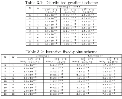
![Figure 3.2: Computing x ∗ and learning b ∗ ( ξ ∼ U [−θ ∗ /2, θ ∗ /2], N = 10)](https://thumb-us.123doks.com/thumbv2/123dok_us/1320511.2676510/88.918.121.807.324.840/figure-computing-learning-ξ-u-θ-θ-n.webp)