Volume 36
Number 589
Egg production functions
Article 1
December 1980
Egg production functions
Earl O. Heady
Iowa State University of Science & Technology
Joseph F. Guinan
Iowa State University of Science & Technology
S. L. Balloun
Iowa State University of Science & Technology
Follow this and additional works at:
http://lib.dr.iastate.edu/researchbulletin
Part of the
Agriculture Commons
,
Animal Sciences Commons
, and the
Economics Commons
This Article is brought to you for free and open access by the Iowa Agricultural and Home Economics Experiment Station Publications at Iowa State University Digital Repository. It has been accepted for inclusion in Research Bulletin (Iowa Agriculture and Home Economics Experiment Station) by an authorized editor of Iowa State University Digital Repository. For more information, please [email protected].
Recommended Citation
Heady, Earl O.; Guinan, Joseph F.; and Balloun, S. L. (1980) "Egg production functions,"Research Bulletin (Iowa Agriculture and Home Economics Experiment Station): Vol. 36 : No. 589 , Article 1.
ECONOMICS &
SOCIOLOGY
READING ROOM
i f? i C « -*r>1
3
Egg Production
Functions
CODEN: IWRBBR(589)1-24(1980) ISSN: 0097-3416Earl 0 . Heady, Joseph F. Guinan, and S. L. Balloun
Center for Agricultural and Rural Development Department of Economics
Department of Animal Science
Agriculture and Home Economics Experiment Station Iowa State University of Science and Technology
CONTENTS
S u m m a ry... 4
In trodu ction ... 5
Experiment u se d ... 5
Egg production patterns over tim e ...6
Production function co n ce p ts... . ... 6
Overall production functions ...8
Estim ated equations... 8
Revised functions for the overall p eriod ... 9
Derived quantities... 9
Functions with time as a variable...10
Derived eq u a tion s...11
Production surface, isoquants, and m arginal rates of substitution... 12
E v a lu a tion ... 14
Corrections for autocorrelation... 14
Regressions on the transformed v a ria b le s... 15
A lternative models of egg production...17
Derived eq u a tion s... 17
Econom ic applications and com parisons... 19
R eferen ces... 23
The E xperim ent Station conducts its program s w ithout discrim ination as to race, color, sex, or na tional origin.
SUMMARY
This study estim ates egg production functions from experim ental d ata The experimental feed variables were com and soybean meal. The experi ment included the four protein levels of 12, 14, 16, and 18 percent and was initiated with 566 birds in 288 cages. Bird density per cage initially was in cluded as a variable, but results were not significant and were dropped from the analysis.
Several algebraic form s were evaluated. For the overall data, a quadratic equation without an in teraction term seemed m ost appropriate. It was used in estim ating egg production, in both numbers and weights for the entire period of the experiment, as a function of com and soybean meal intake. This estimated egg production function then was used in deriving egg isoquants, m arginal rates of substitu tion between feeds, and other quantities that relate to optim izing feed costs.
However, because egg production is an obvious function of stage of lay, production functions also were estim ated with tim e included as a variable. In this situation, egg production and feed inputs were measured over each of 10, 28-day periods. Time was given numbers 1 through 10 for these periods. A quadratic function with interaction terms between com , soybean meal, and tim e seemed most suitable in estim ations of egg production measured in both numbers and weight. Production functions, egg iso quants, and feed substitution equations were derived from the estim ated response equations for the various 28-day time periods. The production func tions possessed the conventional relationships of (a) decreasing m arginal production of feeds at higher egg production levels and (b) decreasing marginal rates of substitution of soybean meal for com at higher protein levels. Productivity of feeds increased over tim e through the fourth week and then
decreased gradually through the remaining six 28- day periods of the experiment.
Exam ination of the quantities estimated from the functions incorporating tim e suggested that they were more suitable in representing the feed-egg pro duction process than were those derived from overall functions w ith time absent. These results parallel those for m ilk production functions where time in the lactation period also proved to be a significant variable.
A utocorrelation is a potential estimational problem for data of the type analyzed. The potential of autocorrelation arises because the same observa tions are used repeatedly. The existence of autocor relation does not bias the mean estimates. It does, however, cloud the interpretation of significance tests and fiducial lim its. Hence, estimates were made after the egg response data were corrected for autocorrelation. Several functional forms based on com , soybean meal, and time variables were evaluated. The functions incorporating corrections for autocorrelation estim ated lower levels of feed in put and egg output per hen than did functions without this m odification. Also, the functions cor rected for autocorrelation provided estimates that better conform with the rise and fall of egg produc tion over the laying period.
Rations that maximize profits per hen above feed costs were derived for several levels of prices for com , soybean meal, and eggs in periods 1, 4, 7, and 10 of the lay period. The optim al ration changes as the relative magnitude of these three prices. The system indicates greater consumption of both feeds with higher egg prices. It also suggests a ration with a somewhat higher percentage of protein as the price of soybean meal is lower relative to the price of com .
Egg Production Functions
1
Earl O. Heady, Joseph F. Guinan, and S. L. BallounFeed is the major cost of producing eggs. Hence, ration formulation, to the extent that it is consistent with profit maximization, should attempt to minimize feed costs for given levels of egg production per hen in a poultry activity.
There are several approaches in minimizing feed costs. One is the linear programming approach of selecting various feedstuffs that w ill minimize feed costs while attaining specified nutrition restraints. The major inform ation needed for this minimizing process includes the prices and the composition of the different feedstuffs and the corresponding nutritional restraints to be attained. A second cost-minimization approach involves equating the marginal rate of sub stitution of the different feeds with their respective price ratios. The major inform ation needed for this minimizing process includes the egg production func tion, the corresponding egg isoquants, the marginal rates of substitution between the feedstuffs, and the prices of the feedstuffs. Actually, the two approaches can use the same data, the programming approach in linear form and the latter in nonlinear form
This study is directed toward the second cost- minimization process. The conditions necessary for this process have been explained elsewhere (Heady and Dillon, 1961). Basic to the process, then, is knowledge of the egg production function or response surface. Hence, the m ajor objective of this study is to estimate egg production functions relative to feed in puts from experim ental data. An auxiliary objective is to apply the production function estimates in deriv ing relevant physical quantities and to make economic applications of them. An important reason for this objective is the fact that egg production func tions have not previously been estimated. Production functions have been estim ated for poultry products, turkeys, and broilers (Askalani, 1970; Balloun et al., 1957; Heady et al., 1956). It is expected, however, that egg production functions should differ from those of turkey and broiler production in somewhat the same manner that m ilk production functions differ from those for beef and pork (Heady et al., 1961).
The variable feeds in the experiment were com and soybean meal. The experim ent included the four protein levels of 12, 14, 16, and 18 percent. Initially, hen housing density, as represented by number of hens per cage, also was included as a variable. Because of few treatm ents used, however, the results were not definitive and are not reported here.
h ’roject 2102 o f the Iow a A griculture and Home Econom ics Ex periment Station, Am es, Iowa.
Experiment Used
The rations were basically com and soybean meal com binations w ith other ingredients held fixed among rations. Their com position is shown in Table 1. Soybean oil was added to keep the energy level constant whenever soybean m eal was substituted for com in raising the protein percentage. Thus the diets were isocaloric, calculated to contain 1,370 m etabolizable calories per pound. Other ingredients remained fixed between rations and accounted for 12.8 percent of the total w eight. W ith minor varia tions, these latter item s are common constituents of layer rations. Of this fixed group for dry matter weight, 6 percent of the total ration was limestone, 3 percent was fish meal, and 2 percent was alfalfa meal. Lim estone is an im portant source of calcium for laying hens. Fish meal and alfalfa are prim arily protein feeds but are usually included in small amounts because they are believed to improve pro duction and egg quality. Results of Kjeldahl tests on pooled samples of each batch of feed are shown at the bottom of Table 1. They indicate that the actual
Table 1, Composition of cations In the experiment Ingredients
Percent of Total Height at Protein Levels 12% 14% 16% 18% Corn (8.6% protein) 81.0 75.5 70.0 64.4 Soybean meal (48.0% protein) 6.0 11.0 16.0 21.0 Fish meal (65.0% protein) 3.0 3.0 3.0 3.0 Alfalfa meal (20.0% protein) 2.0 2.0 2.0 2.0 Dicalcium phosphate 1.0 1.0 1.0 1.0 Limestone 6.0 6.0 6.0 6.0 Salt and trace minerals 0.3 0.3 0.3 0.3 Vitamin mix 0.5 0.5 0.5 0.5 Soybean oil 0.2 0.7 1.2 1.8 Total 100.0 100.0 100.0 100.0 Calculated Analysis
Protein percentage 11.58 13.86 15.60 17.73 Metabolizable' cal* per lb. 1370 1370 1370 1370 S u p p l i e s per pound of ration:
NaCL 1. 2 grams An 20 mg Cu 2.5 Mn 37 mg Fe 15 mg
I2‘ 0.3 Supplies per pound of ration:
Vitamin A 2,300 10 Choline 82 Vitamin D 900 IU Niacine 7 Vitamin
Methionine
2.3 meg Pantothenic acid 2.3 0.05 % Riboflavin 2.3
protein levels were slightly lower than initially calculated for this experiment.
Although bird density per cage also was planned as an experim ental variable, significant differences in perform ance did not prevail among treatments. Hence, the data for the different densities were pooled. Thus, the experim ent was initiated with 566 birds in 288 cages. (The initial experimental design had included treatm ents of one, two, and three birds per cage at each protein level with each of these treatments replicated six tim es.)
The birds were of commercial laying type purchased from a local supplier. At point of lay (ap proxim ately 20 weeks) pullets were weighed, de- beaked, and random ly assigned to the experimental units. An adjustment period of 4 weeks was allowed to enable the birds to adjust to the experimental diets. Lighting was restricted to 13 hours per day at the start but was increased at the rate of 15 minutes every 2 weeks to a maximum of 17 hours per day. Food and water were available ad libitum Heating and ventilation were both provided. Forced air ex haust fans were therm ostatically controlled to main tain a m inimum winter temperature of 50° F. In summer, the fans were capable of moving a max imum of 5 cubic feet of air per hen per minute.
D aily records were kept of egg production and m ortality per experim ental unit. Dead birds were not replaced, so the m ortality data were necessary for an accurate calculation of hen-days and livability index. W eight of eggs produced, average egg weights, and feed consumption per experimental unit were recorded at the beginning and end of the experiment. Average results by 28-day time periods are shown in Table 2.
The experim ental data were used to derive two types of functions: (a) overall functions for the 280-day experim ental period and (b) functions that include tim e as a variable and utilize the monthly (28-day) data. The latter functions have special problem s of estim ation but consider time as a vari able as it relates to the normal decline in egg production as the laying season progresses. In this
Table 2. Egg production, feed consumption and average egg weight per hen over time (pooled data for all observations)
Time Periods (28 days) Number of eggs per 28 hen-days Pounds of eggs per 28 hen-days Pounds of feed per 28 hen-days Average egg wt. (grams) i 21.20 2.53 5.82 54.31 2 21.84 2.71 6.22 56.40 3 21.93 2.79 6.55 57.84 4 21.84 2.83 6.44 58.88 5 20.67 2.70 6.02 59.22 6 20.30 2.67 6.22 60.01 7 19.90 2.65 6.22 60.57 8 19.28 2.59 6.19 61.07 9 18.81 2.53 5.66 61.17 10 18.39 2.45 5.82 60.61
sense, egg production functions parallel those for m ilk production where output also is associated with time in the period of lactation. The overall functions have some intricacies of their own and also are interesting from a m ethodological point of view.
Egg Production Patterns Over Time
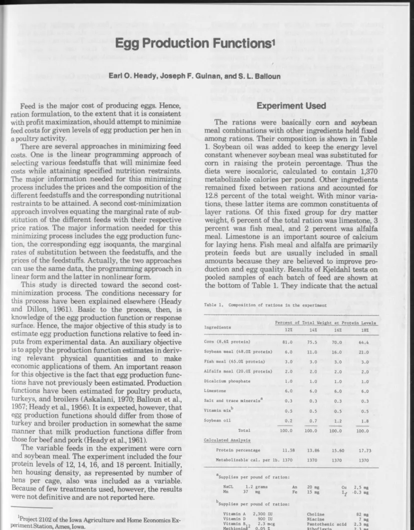
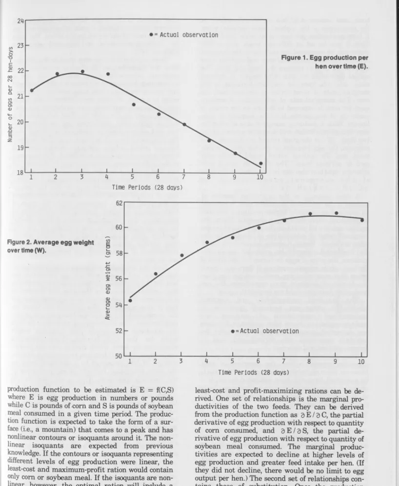
Egg production, like m ilk, follows a characteristic pattern over time. The normal cycle is represented by a curve that rises sharply as the pullets begin to lay, peaks after 8 to 16 weeks, and then falls off until the end of the first season. The particular pattern for the experim ent is shown in Figure 1 for eggs laid. (Pounds of eggs laid and feed intake per hen follow a highly parallel pattern over time.) Average number of eggs per 28 hen-days reached its peak in the third period and then gradually declined.2If total weight of eggs produced, rather than number of eggs, is used as the measure of output, peak production is reached slightly later. This dif ference occurs because average egg weight also in creases as the laying season progresses (Figure 2). Egg weight norm ally increases at a decreasing rate and tends towards an asym ptotic maximum as the birds mature.
Because average egg weight changes over the laying season and has an effect on egg grades and prices, it is desirable also to evaluate egg production on a w eight basis. The tendency for egg weight to in crease with stage of lay causes the production curve not only to peak later but also to fail off at a slower rate during the later months of the laying season. This consideration may be important in response re search and suggests w eight of eggs as an ap propriate measure of production. Consequently, in the later regression work, both number of eggs and pounds of eggs per 28 hen-days are used as measures of output.
Feed consumption also varies over the production cycle. Average intake over all treatments ranged from 5.66 to 6.55 pounds per 28 hen-days during the 10 periods. Beak intake coincided with peak produc tion and tended to decline as the laying season pro gressed.
Production Function Concepts
The concept of the production function is com monly used in econom ic analysis and some biological and physical sciences. The concept and its applica tion to agriculture has been explained in detail elsewhere (Heady, 1952; Heady and Dillon, 1961) and need not be discussed at length here. In this situation, interest is in estim ating egg production as a function of corn and soybean meal (with the qualifications made later in feedstuffs). Hence, the^The curves in Figures 1 and 2 w ere estim ated, using pooled data, by m eans of a grafted polynom ial (after com parison w ith a conven tional quadratic regression). The values of R? for Figures 1 and 2 were 0.9838 and 0.9874, respectively.
24
• = A c tu a l o b s e rv a tio n
Figure 1. Egg production per hen overtim e (E).
Figure 2. Average egg weight over time (W).
Time P e rio d s (28 days)
production function to be estimated is E = f(C,S) where E is egg production in numbers or pounds while C is pounds of corn and S is pounds of soybean meal consumed in a given tim e period. The produc tion function is expected to take the form of a sur face (i.e., a m ountain) that comes to a peak and has nonlinear contours or isoquants around it. The non linear isoquants are expected from previous knowledge. If the contours or isoquants representing different levels of egg production were linear, the least-cost and m axim um -profit ration would contain only com or soybean meal. If the isoquants are non linear, however, the optim al ration w ill include a mix made up of both com and soybean meal.
Once the production function has been estimated, two sets of relationships important for deriving
least-cost and profit-m axim izing rations can be de rived. One set of relationships is the marginal pro ductivities of the two feeds. They can be derived from the production function as 3 E / 3 C, the partial derivative of egg production w ith respect to quantity of com consumed, and 3 E / 3 S , the partial de rivative of egg production w ith respect to quantity of soybean m eal consumed. The marginal produc tivities are expected to decline at higher levels of egg production and greater feed intake per hen. (If they did not decline, there would be no lim it to egg output per hen.) The second set of relationships con tains those of substitution. Once the production function has been estim ated, the isoquants or con tours of the surface can be derived as C = c(S | E) where com is made a function of the amount of
bean m eal consumed (C is a variable dependent on the m agnitude of the soybean meal variable) when E (egg production per hen) is at some fixed level. Thus E can be set at different levels, and an iso quant can be computed for each level. The isoquant denotes the com binations of com and soybean meal that can be used to produce the fixed egg level. The partial derivative for com w ith respect to soybean meal, 9 C / 3 S, from the isoquant equation, is the m arginal rate of substitution of soybean meal for com . The m arginal rate of substitution of soybean meal for com is expected to decline as the ration is made up of the form er (i.e., the isoquant is non linear). W ith a declining m arginal rate of substitu tion, the optim al ration w ill contain a mixture of the two feeds. (If the m arginal rate of substitution were constant, the egg isoquant or contour would be con stant, and the optim al ration would include only com or soybean m eal.) The marginal rate of sub stitution equation also can be computed as the ratio o f t h e m a r g i n a l p r o d u c t i v i t i e s , o r
3 C / 9 S = - O E / 9 S - 9 E / 3 C ) .
A final property of the production function of interest is the isocline or expansion path. It connects all points of successively higher production contours or isoquants where their slopes are equal. Hence, the isocline denotes all points on the isoquants where the m arginal rates of substitution of one feed for the other are equal. Hence, it shows the path over which the feed intake should be expanded as, in this instance, the price of eggs increases but the prices of the feed inputs remain constant. If there is a unique ration that m aximizes egg production per hen, then the fam ily of isoclines that characterize the egg production function would converge at this point.
The m arginal productivities and marginal substitution rates are necessary quantities in m athem atical com putation of least-cost and profit-m axim izing rations. A fter production functions are estim ated quantitatively in this study, the m arginal quantities are derived and used in determ ining optimal rations.
The production functions are estimated as regression equations from the experimental data. However, since egg production functions of the type to be exam ined have not been estimated before, it is necessary to explore alternative mathematical forms of the regression equations that represent the production functions.
Overall Production Functions
In the regressions to follow, egg outputs and feed inputs (dry m atter basis) as aggregates per bird for the entire 280-day period are defined as follows: E = total number of eggs produced per bird, W = total pounds of eggs produced per bird, C = total pounds of corn equivalent consumed per bird, and S = total pounds of soybean meal equivalent consumed per bird.
Soybean meal equivalent, rather than soybean meal alone, is used to allow for protein feeds from
other sources in the ration. Also, com equivalent, in contrast to com alone, makes allowance for the energy content of the soy oil in the ration. The basis for these conversions is explained elsewhere (Guinan, 1972).
Three algebraic form s were fitted to the 280-day data: the Cobb-Douglas (C-D) as in equation (1), a quadratic polynom ial as in equation (2), and a square root function as in equation (5). Quadratic and square root functions have isoclines that con verge to a point, allow ing specification of one ration consistent w ith maximum egg production per bird. This property is desirable to allow definition of a unique ration that maximizes egg production per hen and allow s response elasticity to change over the function. The C-D function lacks this property but is useful where average substitution and transform ation ratios are of interest. The isoquants of the C-D function are asymptotic to the axes for two feed inputs. Also, the isoclines are linear, pass through the origin, and fan out over the feed plane. Thus, this function would suppose that the percen tage of protein in the ration should not be changed as the price of eggs increased while the prices of feeds rem ain constant. Finally, the elasticities of production, the m arginal products of feeds divided by the average products, are constant for the C-D function. This constant elasticity over the produc tion surface seems unlikely in egg production, particularly if a maximum egg production per hen can be derived.
Both the quadratic and square root functions al low peaks, and thus maximum egg production per hen, for the production surface. Under this condition, the isoclines intersect the feed axes and converge at a point over the feed plane where egg production per hen is at a maximum. The isoclines are linear for the quadratic function and nonlinear for the square root function. The elasticities of production for both the quadratic and square root functions, unlike those for the C-D function, have production elasticities for feeds, which change over the produc tion surface. The C-D function requires that each in crement of feed consumed by a hen must result in the same percentage increase in egg production as the previous increment. This is not true for the quadratic and square root functions. Although the square root and quadratic functions are more flexi ble in mathem atical form for the egg production function, all three forms are fitted to the experimen tal data. Then, later, some modified forms of the quadratic function are examined. Detailed charac teristics of these algebraic forms are given elsewhere (Heady and D illon, 1961).
Estimated equations
Equations (1) through (6) show the estimated regression results for each of these functions, using both number of eggs (E) and w eight of eggs (W ) as de pendent variables.
w
= 0.730C06528 S02999 (2) E = 2133.144 - 69.844C - 75.583S + 0.609C2 + 0.490S2 + 1.522SC (3) W = 331.715 -11.007C - 12.429S + 0.095C2 + 0.077S2 + 0.252SC (4) E = 8594.688 + 119.019C + 25.736S - 2020.215C05 - 1059.212S05 + 136.435S05C05 (5) W = 1536.144 + 21.156C + 4.642S-361.463C05 -194.114S05 + 24.984Sa5 C05 (6)Table 3 shows the t values of the coefficients and the R2 values obtained from these regressions. Between two-thirds and four-fifths of the total varia tion in egg production was explained, depending on the type of function and the measure of production used. The Cobb-Douglas function results in highly significant regression coefficients. W ith the exception of this function, however, t values for coefficients of other algebraic forms are weak, being significant mostly at probability levels of 0.2 to 0.3.
Revised functions for the overall period
If the CS interaction term is dropped from the quadratic as estimated by equations (3) and (4), equa tions (7) and (8) result. Sim ilarly, if the interaction term is dropped from the square root functions, equa tions (9) and (10) result. The purely linear form is estimated as (11) and (12), respectively, for egg and weight outputs. E = -276.505 + 14.509C + 9.560S - 0.125C2 - 0.203S2 (7) W = -67.183 + 2.957C + 1.665S - 0.026C2 -0.037S2 (8) E = -1194.034-21.459C -3.427S -I- 330.788C05 + 54.992S05 (9) W = -256.389 - 4.568C - 0.698S + 69.058Ca5 + 9.921S05 (10) E = 81.538 + 1.734C + 3.829S (11) W = 6.651 + 0.287C + 0.593S (12)
The coefficients of the revised quadratic and square root equations generally bear the expected signs, indicating dim inishing marginal productivity of the two feeds in egg production. Also the t values of the coefficients improve somewhat, as shown in Table 4. The values of R2 decline slightly but not significantly.
Derived quantities
Since equation (8) seems statistically to be one of the better fits, quantities of economic importance are derived from it. Equation (8) has as large an R2 as the other equations and has sm aller negative constants or more logical signs on other estimated coefficients. Further m odifications in the form and improvement in estimated statistics are accomplished later in the manuscript. Equations (13) through (16), derived from equation (8), show the marginal productivity, isoquant, and m arginal rate of substitution equations derived from equation (8).
2
Table 3. R and t values for equations (1) through (6) Equation
R2
Value of t in order of coefficient in equation b0 bl b2 b3 b4 b5 O ) 0.6791 2.724 2.596 4.858 (2) 0.7347 0.305 3.161 5.516 (3) 0.7435 1.205 1.118 1.229 1.109 0.938 1.387 (4) 0.7923 1.389 1.307 1.499 1.287 1.098 1.703 (5) 0.7415 1.148 1.089 1.118 1.115 1.260 1.327 (6) 0.7945 1.536 1.449 1.510 1.494 1.729 1.820 Table 4. R and t values2 for equations (7) through. (12)
Equation
Value of t in order of coefficient in equation R2 b0 b l b 2 b 3 b4 (7) 0.7162 0.789 1.000 2.533 0.834 1.293 (8) 0.7589 1.388 1.475 3.196 1.269 1.727 (9) 0.7163 0.906 0.767 0.491 0.852 1.208 (10) 0.7556 1.402 1.177 0.721 1.282 1.571 (11) 0.6519 1.542 1.843 4.113 (12) 0.6510 0.839 2.031 4.251 9 W / d C = 2.957 - 0.052C (13) d W / d S = 1.665-0.074S (14) C = 56.865 ± [19.231 (1.757 + 0.173S - 0.004S2 - 0.104W )05] (15) d C / a S = [1.665 - 0.074S] / [2.957 - 0.052C] (16)
The m arginal productivity equation for com in (13) indicates the increm ent in egg production from an increm ent in com intake, other inputs held con stant. Equation (14) is the marginal productivity of soybean meal and indicates the increment in egg pro duction from an increm ent in intake of soybean meal. The isoquant equation (15) defines all combinations of com and soybean m eal that w ill produce a given (equal) quantity of egg w eight per hen. The isocline equation indicates all corn-soybean meal combina tions that have exactly the same substitution ratio of soybean m eal for com as egg production moves to higher levels. These concepts are explained in detail elsewhere (Heady and Dillon, 1961).
An obvious effect of dropping the interaction term in equation (8) is that all derived equations are sim plified. The isoquant equation is modified by the loss of an S term, w hile the truncated marginal pro ductivity equations give rise to much simplified m arginal rate of substitution equations. Conse quently, isoclines derived from equation (15) also are modified, and the ridgelines become perpendicular to the axes. Figure 3 shows the net result of these restrictions for isoquants of 22, 25, and 28 pounds of eggs as derived from equation (8). Four isoclines, cor responding to m arginal substitution rates of soybean meal for corn of 0.5, 1.0, 2.0, and 3.0 also are shown. These isoclines converge to the point (22.5, 56.9) that denotes maximum egg production per bird if equation (16) is used for prediction. The ridgelines fall perpen dicular to their axes from this point. Some sample
iso-Pounds o f soybean meal per hen (280 days)
Figure 3. Isoquants, isoclines, and ridgelines for re vised quadratic production function (8) (egg weights produced in 280 days).
quants and m arginal rates of feed substitution are in cluded in Table 5. The pairs of quantities of the two feeds Under each level of egg production represent the egg isoquant. The m arginal rates of substitution between the two feeds, 3 0 / 3 S, correspond with the feed pairs shown for each egg production level per hen. The percentage of protein is calculated for the feed quantities under each production level.
Functions With Time as a Variable
Because tim e (stage of lay) is an important vari able affecting egg production levels, functions were estim ated that include time as an explanatory vari able. In these regressions, the variables are defined as follows: E = total number of eggs produced per bird per 28 days, W = total pounds of eggs produced per bird per 28 days, C = total pounds of corn equivalent consumed per bird per 28 days, S = total pounds of soybean meal equivalent consumed per bird per 28 days, and T = time' in 28-day periods measured by the numbers 1 through 10. Four forms of functions were estim ated for both dependent variables (E and W). The results are given in equa tions (17) through (24). The first three pairs consist of Cobb-Douglas, quadratic, and square root equa tions, respectively. The last pair is an adaptation of a function found to give good results in m ilk produc tion (Heady et al., 1961). Both these functions allow interaction between tim e and the squared term for each feed ingredient. O f course, both allow dim inishing marginal productivity of feedstuffs, changing elasticities of production with greater egg weight per hen, and dim inishing marginal rate of substitution of each feed for the other as the com position of the ration changes. Too, the equations have isoclines that intersect over the feed plane at the feed com binations that maximize egg production per hen. g _ g 798C°-53°5 g0.2334 rp-0.0605 (17) W = 1.066C0 5927 S02642 T-00078 (18) E = -4.0164 + 6.6423C + 5.3157S + 0.3745T - 0.5282C2 - 1.3238S2 - 0.0007T2 + 0.5630CS - 0.1106CT - 0.1889ST (19)Table 5. Feed combinations per hen and marginal rates of substitution derived from quadratic equation (8) (egg weight produced in 280 days)
22 lbs, eggs_________ ________ 25 lbs, eggs_________ ______ 28 lbs, eggs Lbs. soy bean meal Lbs. corn 3C/3S Protein % Lbs. soy bean meal Lbs. corn 3C/3S Protein % Lbs. soy bean meal Lbs. corn 3 C/3 S Protein % 4.0 50.9 4.39 10.6 5.0 47.6 2.68 11.6 6.0 45.3 2.03 12.2 6.0 52.5 5.41 11.7 7.0 43.5 1.65 13.0 7.0 48.9 2.77 12.5 8.0 42.0 1.39 13.7 8.0 46.6 2.01 13.3 9.0 40.8 1.19 14.5 9.0 44.9 1.60 14.0 9.0 51.5 3.58 13.3 10.0 39.7 1.03 15.2 10.0 43.4 1.32 14.7 10.0 48.8 2.21 14.1 11.0 38.7 0.90 16.0 11.0 42.3 1.12 15.4 11.0 47.0 1.66 14.8 12.0 37.9a 0.79 16.7 12.0 41.3 0.96 16.1 12.0 45.6 1.32 15.5 13.0 37.2a 0.69 17.3 13.0 40.4 0.82 16.8 13.0 44.4 1.09 16.2 14.0 39.7 0.71 17.4 14.0 43.5 0.91 16.8 15.0 39.1 0.60 18.0 15.0 42.7 0.76 17.4 16.0 38.6 0.51 18.6 16.0 42.1 0.63 17.9 17.0 41.6 0.51 18.5 18.0 41.2 0.41 19.0
W = -1.0931 + 0.9207C + 0.7028S + 0.1312T - 0.0765C2 - 0.2553S2 - 0.0042T2 + 0.1321CS - 0.0146CT - 0.0262ST (20) E = -62.2865 - 10.7807C - 2.0212S - 0.3397T + 55.7759C05 + 8.8787S05 + 7.3127T05 + 3.4270C05S05 - 2.5357C05T °5 - 1.8136S05T °5 (21) W = -4.9589 - 1.1013C - 0.4526S - 0.0928T + 4.8045C05 - 0.3302S05 + 0.8615T° 5 + 1.3242C05S05 - 0.1555C05T 05 - 0.1708S05T °5 (22) E = 6.1679 + 2.2977C + 4.9598S + 0.1007T - 0.0145C T - 0.1022S*T (23) W = -0.0357 + 0.4001C + 0.8060S + 0.0537T - 0.0020CT - O .O lôlS ^ (24)
Although the variable tim e in the stage of lay, T, has been added, the foregoing equations still have the mathematical characteristics mentioned pre viously. The C-D function has linear isoclines through the origin, does not define a unique ration to maximize egg production per hen, and has con stant elasticities of production. The other algebraic forms have isoclines that converge at maximum egg production per hen w hile production elasticity is not constant. Isoclines for the quadratic form are linear while those for the square root forms are not.
Table 6 shows the R2 and t values of the coeffi cients obtained in the preceding regressions. The quadratic and square root equations explained about three-quarters of the variance in number of eggs produced per bird per 28-day period. The Cobb- Douglas equations explained a smaller proportion of the variation but gave higher t values. Nevertheless, the Cobb-Douglas equation is not used for analysis purposes because of its mathematical properties. It forces the isoclines to be linear and pass through the origin of the feed plane. Consequently, the optimal ration would not change w ith the level of egg pro duction per hen under a given price ratio for com
and soybean meal. Also, this function has constant elasticities of production and no unique feed com bination that maximizes egg production per hen. On the basis of t value and R2 criteria, we m ight select equation (23) as an appropriate prediction equation for num ber of eggs. It should also be kept in mind that the t values for the estimated coefficients, although not biased, have questionable interpreta tions owing to potential autocorrelation. Repeated observations were taken on the same experimental units and, hence, cannot be regarded as independent (i.e., measurements for the same birds were taken in subsequent 28-day periods). It has been pointed out (Puller, 1968) that, although possible autocorrela tion does not bias the coefficients, it does affect the t tests.
From a logical consideration of egg production response, it is likely that the quadratic function would be chosen. It has changing elasticities as egg production per hen increases and gives optimal ra tions that change w ith higher levels of egg produc tion. The square root function has similar properties in that it allows a single maximum to be reached and gives isoclines that allow changing ration specifications as higher levels of production are at tained. These conditions exist because the isoclines converge at the peak of the surface and do not in tersect the origin of the feed plane. These functions also allow full interaction of the ration ingredients C and S w ith time. However, the coefficient on the SP-5 term in equation (22) is negative, im plying in creasing returns to soybean meal. Hence, the quadratic equations (19) and (20) are selected for estim ating egg production surfaces, feed substitution rates, and other relevant quantities.
Derived equations
Equations (19) and (20) are used to predict feed com binations and m arginal rates of substitution of soybean m eal for corn for various isoquant levels in selected m onths (28-day periods) of the experiment.
Table 6. _2R and t values for equations (17) through (24)
Equation R2
Value of t in order of coefficient in equation3
b0 bi b2 b3 b4 b5 b6 b7 b8 b9 (17) 0.6794 30.867 11.185 18.142 13.714 (18) 0.6182 0.801 11.635 19.124 1.645 (19) Q.7505 0.213 1.033 0.798 0.791 0.963 1.769 0.069 0.494 1.306 2.106 (20) 0.6603 0.409 1.010 0.744 1.954 0.983 2.405 3.1Ì0 0.818 1.216 2.062 (21) 0.7515 0.843 1.051 0.631 1.871 1.015 0.330 1.856 0.343 1.607 2.250 (22) 0.6625 0.473 0.758 0.997 3.608 0.617 0.086 1.543 0.935 0.695 1.495 (23) 0.7381 2.591 5.277 10.266 2.550 1.922 3.135 (24) 0.6092 0.101 6.177 11.217 1.975 1.820 3.323
aA t value of 1.97 Is significant at the 0.05 level.
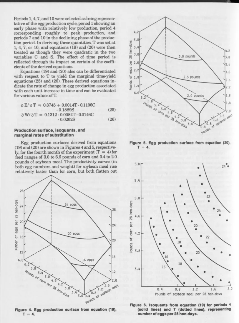
Periods 1 ,4 ,7 , and 10 were selected as being represen tative of the egg production cycle; period 1 showing an early phase w ith relatively low production, period 4 corresponding roughly to peak production, and periods 7 and 10 in the declining phase of the produc tion period. In deriving these quantities, T was set at 1, 4, 7, or 10, and equations (19) and (20) were then treated as though they were quadratic in the two variables Ç and S. The effect of time period is reflected through its im pact on certain of the coeffi cients of the derived equations.
Equations (19) and (20) also can be differentiated with respect to T to yield the marginal tim e-yield equations (25) and (26). These derived equations in dicate the rate of change in egg production associated with each unit increase in tim e and can be evaluated for various values of T.
3 E / 3 T = 0.3745 + 0.0014T - 0.1106C
-0.1889S (25)
3 W / 3 T = 0.1312-0.0084T -0.0146C
- 0.0262S (26)
Production surface, isoquants, and marginal rates of substitution
Egg production surfaces derived from equations (19) and (20) are shown in Figures 4 and 5, respective ly, for the fourth month of the experiment (T = 4) for feed ranges of 3.0 to 6.6 pounds of com and 0.4 to 2.0 pounds of soybean meal. The productivity curves (in both egg numbers and w eight) for soybean meal rise relatively faster than for com , but both flatten out
Figure 4. Egg production surface from equation (19), T = 4.
Figure 5. Egg production surface from equation (20), T = 4,
Pounds o f soybean meal per 28 hen-days
Figure 6. Isoquants from equation (19) for periods 4 (solid lines) and 7 (dotted lines), representing number of eggs per 28 hen-days.
rather quickly. In Figure 4 these isoquants represent number of eggs, while in Figure 5 they are in terms of pounds of eggs per bird.
Tables 7 and 8 show feed combinations and marginal rates of substitution for several output levels derived from equations (19) and (20), respec tively. Both tables are calculated for the fourth period. M arginal substitution rates, 3 C/ 3 S, tend to be higher in Table 8, if the 2.50-pound isoquant is con sidered to correspond approxim ately with the 18-egg isoquant in Table 7.
Isoquants for the fourth and seventh periods de rived from equation (19) are presented in Figure 6.
Equal increm ents of output are represented between successive isoquants; in this case, two eggs per hen per 28 days. For either tim e period, the increasing dis tance between successive isoquants is indicative of decreasing returns to feed. Also, isoquants for specific egg levels lie further to the right in period 7 than in period 4. In other words, after the peak is reached, about period 4, more of any ration combination is needed to produce a given quantity of output as the stage of lay (tim e) increases. W ithin the feed ranges shown, the 24-egg isoquant is ju st attainable in the seventh month.
The egg contours also display greater curvature at
Table 7. Feed combinations and marginal rates of substitution derived from quadratic equation (19) (T *■ 4) for egg numbers
Level of Pounds of cor n required to Marginal rates of substitution soybean m a i n t a i n egg output per (3C/3S) along egg
meal h e n per 28 days of isoquant of
(lbs. per 28 18 20 22 18 20 22
hen-days) eggs eggs eggs eggs eggs eggs
0.6 4.25 2.62 0.7 4.02 5.16 2.11 4.92 0.8 3.82 4.77 1.76 3.19 0.9 3.66 4.50 1.49 2.41 1.0 3.52 4.28 5.56 1.28 1.93 5.65 1.1 3.40 4.11 5.14 1.11 1.60 3.26 1.2 3.30 3.96 4.86 0.96 1.34 2.37 1.3 3.21 3.84 4.65 0.83 1.14 1.85 1.4 3.73 4.49 0.97 1.50 1.5 3.64 4.35 0.83 1.24 1.6 3.57 4.24 0.70 1.03 1.7 3.50 4.14 0.59 0.86 1.8 4.06 0.71 1.9 4.00 0.59 2.0 3.95 0.47
Table 8. Feed combinations and marginal rates of substitution derived from quadratic equation (20) (T * 4) for egg weights
Level of Pounds of corn required to Marginal rate of substitution soybean m a i n t a i n egg output per (3 C/3 S) alo n g egg
m e a l h e n per 28 days of isoquant of
(lb's, per 28 2.50 2.75 3.00 2.50 2.75 3.00 hen-days) l b s . l b s . l b s . l b s . l b s . l b s . 0.6 5.54 10.96 0.7 4.90 4.34 0.8 4.55 2.91 0.9 4.30 5.32 2.18 5.01 1.0 4.11 4.93 1.72 3.08 1.1 3.95 4.76 5.95 1.39 2.23 8.42 1.2 3.83 4.47 5.42 1.13 1.71 3.66 1.3 3.72 4.32 5.12 0.92 1.35 2.44 1.4 3.64 4.20 4.91 0.74 1.08 1.80 1.5 3.58 4.10 4.76 0.59 0.87 1.38 1.6 3.52 4.03 4.63 0.46 0.68 1.08 1.7 3.97 4.54 0.53 0.84 1.8 3.92 4.47 0.39 0.64 1.9 3.89 4.41 0.27 0.48 2.0 3.87 4.37 0.16 0.34 13
higher production levels, indicating that, as feeding levels increase, sm aller ranges of feed combinations w ill allow a specified level of egg production. In the lim it of production, at the point of isocline con vergence, only one feed com bination would allow maximum egg production per bird. It also is evident that, as tim e progresses, the same isoquant, such as 20 eggs, becom es more curved. This greater curvature reflects the more rapid changes in substitution rates as feed proportions are varied in attaining that out put level.
Evaluation
The preceding sections have examined functions for both the overall and 28-day data The search for an overall function based on ration ingredients proved less than satisfactory just as it did in the m ilk and other studies reported elsewhere (Heady and Dillon, 1961). The prim ary objective of the study was to find a suitable prediction equation for egg production by commercial layers during their first season of production. W ith the production function appropriately estimated, it is possible to determine how rations should change as the prices of either the feeds or the eggs change. W hen the 28-day data were used, equations (19) and (20) were selected as perhaps best for this purpose, in terms of both R2 and t values. Both are quadratic type functions based on ration ingredients and time or stage of lay. They are sim ilar in form except that equation (19) uses num ber of eggs (hen-day production) as its in dex of output while equation (20) uses pounds of eggs. W e now turn to some statistical problems re lating to the estim ation of these functions.
Corrections for Autocorrelation
As has been m entioned previously (Fuller, 1968), repeated measurements on the same bird or pen of birds give rise to the potential of autocorrelation and cloud the interpretation of significance tests. Although this procedure does not bias the mean estimates, we know little about the fiducial lim its that conform to them. Accordingly, this section is de voted to resolution of these difficulties for the egg experim ental dataSuccessive measurements on the same birds violate the concept of independence among observa tions basic to classical statistical tests. However, ex perim ental designs that use each bird or animal for a single observation for the complex rations, feed in puts, and gains and then discard it would be very costly. Hence, there is need to correct for this situa tion so that data of the type used for the laying hens can be used effectively for economic decisions. In ad dition to the problem of repeated observations with the same birds or animals, there also is the problem of ad libitum feeding. W hen animals have free ac cess to feed, either the tim e intervals at which ob servations are taken or the quantity of feed con sumed can be fixed. But it is not possible to control
both sim ultaneously. In the conventional experi ment, observations on production and feed consump tion are taken at fixed intervals. Where animals are self-fed w ith continuous access to feed, the amount of feed consumed, determ ined by the animal, is en dogenous. Hence, use of feed quantity as an indepen dent variable violates least squares assumptions since feed consumption is not fixed but is measured with error. Hence, production coefficients estimated in this way can be biased. Fuller (1968) illustrates reduction of the bias by using means of several replicates instead of the individual observations. Thus, we proceed to make these corrections for the egg data.
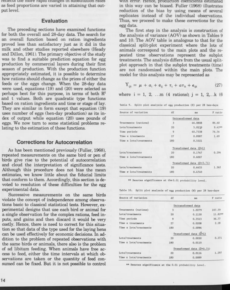
The first step in the analysis is construction of the analysis of variance (AOV) as shown in Tables 9 and 10. The AO V table is analogous to that for the classical split-plot experim ent where the lots of animals correspond to the main plots and the re peated time observations represent the subplot treatments. The analysis differs from the usual split- plot approach in that the subplot treatments (time) are not randomized w ithin the main plots. The model for this analysis may be represented as
Y ijt = /a + cti + e*j + r t + a r it -I- €ijt (27)
where i = 1, 2, ....m (4 rations); j = 1, 2 ,...k (6 Table 9. Split plot analysis of egg production (E) per 28 hen-days, Source of variation df ms F ratio
Untransformed data Treatments (rations) 3 46.0808 86.60 Lots/treatments 20 5.013(9 9.42** Time periods 9 40.7338 76.56 Time x treatments 27 0.8987 1.69 Time x lots/treatments 180 0.5321 Transformed data (0“ 1) Lots/treatments 20 0.1767 0.294 Time x lots/treatments 180 0.6007 Transformed data (¡3=0. 71) Lots/treatments 20 0.6455 1.362 Time X'lots/treatments 180 0.4740
** Denotes significance at the 0.01 probability level Table 10* Split plot analysis of' egg production (W) per 281 hen-days Source of variation df ms F ratio
Untransformed data Treatments (rations) 3 1.0279 107.59 Lots/treatments 20 0.1130 11.82** Time periods 9 0.3513 36.77 Time x treatments 27 0.0208 2.18 Time x lots/treatments 180 0.0096 Transformed data (p=l) Lots/treatments 20 0.0030 0.271 Time x lots/treatments 180 0.0110 Transformed data (¡3=0. 75) Lots/treatments 20 0.0116 1.297 Time x lots/treatments 180 0.0089
replicates); t = 1 ,2 ,.. .N (10 tim e periods); Y ijt = egg production per hen (E or W ) for the t 28-day period of lot j receiving treatm ent i; fx = overall mean; q = treatm ent (ration) effects; e^ = error as sociated with lot j w ithin treatment i; rt = time ef fects; a T it = time by treatm ent interaction; and
fejt = error associated w ith time.
We do not expect successive production and feed observations on the same lot of birds to be indepen dent. Experimental units with higher than average egg production in one period are likely to be similar in succeeding periods. Some units w ill have con sistently high feed intake levels, while others show equally consistent low feed consumption throughout the entire laying season. The resulting correlation or dependence is expressed in the split-plot model as a lot component as seen in Table 9. In previous ex periments dealing w ith m eat animals, taking first differences (or pseudo differences based on the estimated autocorrelation coefficient p ) resulted in the removal of this lot component. In this study p was estimated by 4 6 10 j 5 , £ t <Y,jt,- Y lt, ) p = -- ---4 6 10 f c , < Y * , - W (28)
where Y ijt = egg production per hen at time t of lot j receiving treatm ent i; and Yi t = mean egg produc tion per hen at tim e t of the lots receiving treatment i. The estim ated values for p were 0.7102 for number of eggs (E) and 0.7485 for w eight of eggs (W). By us ing these values for p, the data were transformed as
Pd, = Y Ym-p Y m (29)
and the AOV was repeated for the transformed data The result for number of eggs (E) is shown in Ta ble 9 and for the weight of eggs (W) in Table 10. For number of eggs, the autocorrelation transformation reduced the ratio of the mean square for lots within treatments to the mean square for time by lots within treatments from 9.42 for the original data to 1.362 for the transformed data The corresponding ratios for W were 11.82 and 1.297. U sing the simple first-order autoregressive model w ith p = 1 (first differences), as was done in previous experiments for meat animals, we reduced this ratio to 0.294 for E and 0.271 for W. In other words, the autocorrelation transforma tion using the estim ated p values effectively removed the lot com ponent of error in the model. Since the F ratio for lots/treatm ents was no longer significant, the error component for lots was assumed equal to zero, and the errors were pooled. Hence, our best estimate of a2 is 0.0092 for W and 0.4911 for E. In passing, we note from Tables 9 and 10 that the F ratios for lot/treatm ents are significant, so the hypothesis that all the treatments are alike is re jected.
U nfortunately, the egg data do not permit a test of the adequacy of the overall quadratic model.3 However, the data do allow the test of the hypothesis that the quadratic function in C and S may be used to represent production throughout the range of the ex periment. To conform w ith equations (19) and (20), we modify the analysis at this stage to incorporate time, T, directly into the equation. The analysis im plicitly assumes that the tim e mean square may contain two components. One is a treatm ent component as sociated w ith feed consumption, the other a random component due m ainly to environmental dis turbances. Temperature or humidity common to a particular tim e may affect egg production of all lots alike. The fixed or treatm ent component is expected to be explained by the production surface. If a signifi cant lack of fit shows up, we may conclude either that the functional form is inadequate or that sizable ran dom tim e effects are present.
Regressions on the transformed variables
By using the 40 means of the experiment, the follow ing regression m odel was fitted;
Y ,t == /3o + /3 A , -I- ftS i.t + /I3T
+ m J + ftS u * + /^t2 + 0tCSu + /3aCTlt
+ ftS T i.+ i . a,D, (30)
t = 1
where all the variables except T, T2, and Dt were first transformed as in equation (29). For example
Y u = T u -p Y ta
bui = Cu-pC%
(31)
c \t = C V p C 2iw .etc.
T and T2 represent tim e in 28-day periods as in equa tions (19) and (20). To test if the functional form used in these equations was adequate, especially as to the time variables specified (nam ely, T and T2), a remain ing set of variables to the lim it allowed by the 10 periods of the experim ent was introduced. Accord
ingly, Dt represents a set of dummy variables with zero means for the rem aining 7 degrees of freedom as sociated w ith tim e effects.
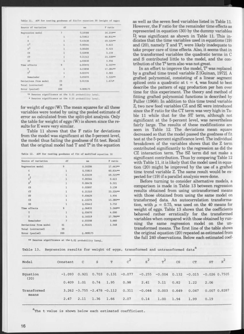
The regression was first computed with all variables and then w ith the tim e effects T, T 2, and Dt removed. First the higher order time effects Dt were dropped, then T2, and, finally, after T was dropped, the model was fitted using the feed variables C through ST alone. Then the A O V in Table 11 was constructed
"T he general tw o-variable quadratic requires that we estim ate a m inim um of five param eters assum ing the constant term zero. A goodness o f fit test, therefore, requires at least six independent ob servations or treatm ents. The egg experim ent had only four rations, allow ing the testin g of a three-param eter m odel for the overall func tion.
Table 11. AOV for testing goodness of fit for equation 3Q (weight of eggs; Source of variation df ms F ratio Regression model 7 0.18588 20.259** c 1 0.55812 60.831** S 1 0.45438 49.524** c2 1 0.00564 0.615 s2 1 0.00480 0.523 cs 1 0.02898 3.159 CT 1 0.21312 23.228** ST 1 0.03630 3.956 Time effects 9 0.05970 6.507** T 1 0.15858 17.284** T2 1 0.02370 2.583 Remainder 7 0.05070 5.526** Deviations from model 23 0.01536 1.674* Total (corrected) 39
Error (pooled) 200 0.009175 ** Denotes significance at the 0.01 probability level.
* Denotes significance at the 0.05 probability level.
for w eight of eggs (W). The mean squares for all these variables were tested by using the pooled estimate of error as calculated from the split-plot analysis. Only the table for w eight of eggs (W ) is shown since the re sults for E were very similar.
Table 11 shows that the F ratio for deviations from the m odel was significant at the 5-percent level, the model thus failing the goodness of fit test. Recall that the original model had T and T 2 in the equation
Table 12. AOV for testing goodness of fit of modified equationi 30 Source of variation df ms F ratio Regression model 9 0.16206 17.663** C 1 Q. 55815 60.834** S 1 Q.45439 49.525** c2 1 0.00564 0.615 s2 1 0.. 00478 0.521 cs 1 0.02897 3.158 CT 1 Q. 21310 23.226** ST 1 0.03629 3.956 CZ 1 0.12276 13.380** SZ 1 0.03443 3.752 Time effects 9 Q.04833 5.268** T 1 Q. 03670 4.000 Z 1 Q. 16319 17.786** Remainder 7 0.03358 3.660 Deviations from model 21 0.01421 1.548 Total (corrected) 39
Error (pooled) 200 0.009175 ** Denotes significance at the Q..Q1 probability level,
as w ell as the seven feed variables listed in Table 11. However, the F ratio for the remainder time effects as represented in equation (30) by the dummy variables Dt was significant as shown in Table 11. This in dicates that the time variables used in equations (19) and (20), nam ely T and T2, were likely inadequate to take proper care of tim e effects. Also, it seems that in the transform ed variables the quadratic terms in C and S contributed little to the model, and the con tribution of the T2 term also was not great.
In an effort to improve the model, T2 was replaced by a grafted tim e trend variable Z [Guinan, 1972]. A grafted polynom ial, consisting of a linear segment spliced onto a quadratic at t = 4, was found to best describe the pattern of egg production per hen over time for this experiment. The theory and method of fitting grafted polynom ial functions is described by Fuller (1968). In addition to this time trend variable Z, two new feed variables CZ and SZ were introduced since the F ratio for the CT term was very high in Ta ble 11 w hile that for the ST term, although not significant at the 5-percent level, was nevertheless fairly large. The results of these modifications are seen in Table 12. The deviations mean square decreased so that the model passed the goodness of fit test at the 5-percent significance level. The individual breakdown of the variables shows that the Z term contributed significantly to the regression as did the CZ interaction term. The SZ term did not make a significant contribution. Thus by comparing Table 12 with Table 11, it is likely that the model used in equa tion (20) m ight be improved by the use of a grafted time trend variable Z. The same result would be ex pected for (19) if a parallel analysis were done.
Before turning to consider alternative models, a comparison is made in Table 13 between regression results obtained from using untransformed means with those obtained from using the same model on transform ed data. An autocorrelation transforma tion, w ith p = 0.75, was used on the 40 means for weight of eggs. Table 13 shows that the coefficients behaved rather erratically for the transformed variables when compared w ith those obtained by run ning the same regression model on the un transformed means. The first line of the table shows the original equation (20) repeated as estimated from the full 240 observations. Below each estimated
coef-Table 13. Regression results for weight of eggs, transformed and untransformed data
Model Constant C S T c
2
s2
T2 CS CT ST R2 Equation -1.093 0.921 0.703 0.131 -0.077 -0.255 -0.004 0.132 -0.015 -0.026 0.7505 (20) 0.409 1.01 0.74 1.95 0.98 2.41 3.11 0.82 1.22 2.06 Transformed 3.262 -3.755 -2.478 -0.112 0.311 -0.044 0.003 0.649 0.047 0.007 0.8287 means 2.47 2.11 1.36 1.66 2.07 0.14 1.00 1.94 1.99 0.19ficient its t value is shown. The second line shows the equation estimated by using the same model on the 40 transformed means.
The poor correspondence between the equations estimated from the transform ed data and the other two equations suggests that a problem of near singularity in the X m atrix may exist. Hence, an at tempt was made to find a function that would require estimation of fewer feed variables and still ade quately describe the production process.
Alternative models of egg production
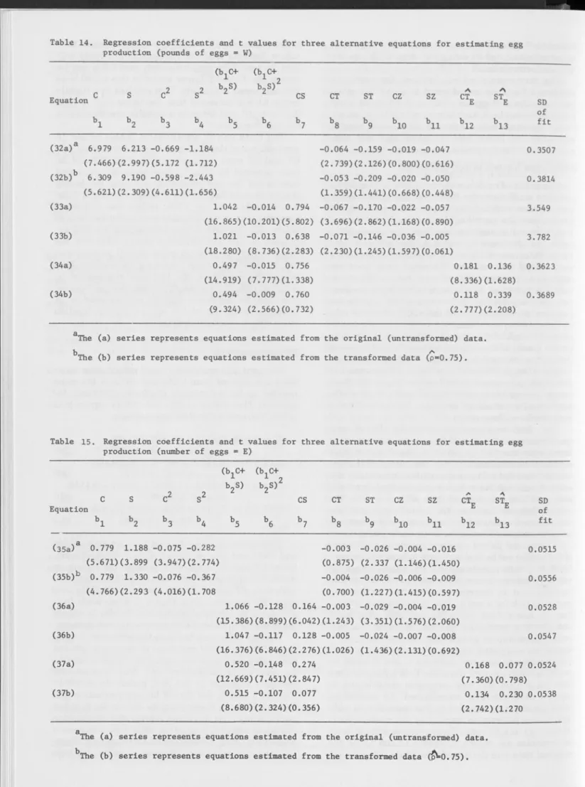
A number of models were tried that attempted to estimate coefficients for fewer feed variables since it was felt that with only four rations this source could have caused the near-singular matrix. Three of these models are discussed because they are interrelated and trace the steps by which a final selection was made. To conserve degrees of freedom, these models were fitted without an intercept since previous regressions indicated that an intercept was not essen tial. The intercept or constant in the equation does not affect the partial derivatives, which express the marginal productivities and the marginal rate of sub stitution of the feeds. Tables 14 and 15 list the coeffi cients for each of the three models as estimated from (a) the means of the original untransformed data and (b) the transformed data means. Table 14 deals with weight of eggs (W), whereas Table 15 presents the corresponding estim ates for number of eggs (E). The t values are given in parentheses below their coeffi cients, and the standard deviation (SD) of the fit also is shown for each equation.
The first equation involves the linear and quadratic term s in C and S and the interaction of these with the time trend variables, T and Z. This equation was estim ated from the means of the un transformed data. The next equation has exactly the same functioned form but was estimated from the means of the transformed data with p = 0.75. The correspondence between the transformed and un transformed estim ates is obvious although there was a slightly higher SD of fit for the transformed data.
The second pair of equations used the coefficients of C and S from the first equation to form a new varia ble (fyc + b
2
S) and its square. Use of this composite variable reduces by one the number of coefficients to be estimated. It, therefore, represents a further step in our search for a model that would require estima tion of fewer feed variables and still adequately describe the production process. However, the pro cedure does impose a restriction on how the C and S terms are estim ated since a proportionality or fixed relationship is assumed between C and S based on coefficients estim ated from the first equation. Care was taken that this new composite variable and its square were correctly transformed. An interaction term CS also was included in this regression in addi tion to the interaction im plied by the cross-products of the (bjC 4- baS)2 term. The results of using this set of variables are shown in Tables 14 and 15 for the original data and the transform ed data. The functionis acceptable since the signs are appropriate and the t values indicate that the coefficients are fairly reli able. To test if the proportionality restriction was too severe, the C and S linear terms in this model were also estim ated separately. This resulted in a slightly better fit but indicated that the terms (bxC + baS), (fyC + baS)2, and CS gave a suitable specification of the feed variables.
The third pair of equations in Tables 14 and 15 were estim ated exactly like the second set except that CT and CZ were replaced by CT& while ST and SZ were replaced by STE. T E represents the estimated time trend for egg production (E) over the laying season as described by the grafted polynomial func tion described earlier. Thus, in this last functional form, the first three variables are exactly the same as before, but the time x feed interactions are now ex pressed by the two variables shown. However, the function did not perform quite so well as equations (33) and (36) in terms of t values of the coefficients or overall fit. Therefore, the functions represented by equation (33b) for the weight of eggs (W) and by equa tion (36b) for number of eggs (E) were selected as ap propriate estim ates of the egg production function given that we had only four rations.
Derived equations
Isoquant and m arginal rate of substitution equa tions are derived from (33b) and (36b) in the same manner as for the original quadratic equations (19) and (20). They follow in (38) and (39) for egg weights and in (40) and (41) and for egg numbers:
C = 7.919-0 .8 3 7 S ± (-1.767) [20.088 + 5.68IS - 1.011S2 - 1.132E]05 (38) a C / d S = [8.772 -0.218S - 0.474CH4.482 -0.566C -0.747S] (39) C = 9.417 -0.833S ± (-20.833) [0.204 + 0.115S
-
0
.
027
s
2
-o.o96W]°5
(40)
a O d S = [1.570 - 0.592S - 0.040Cy[0.452 - 0.048C - 0.040S] (41)Production surfaces derived from equations (33b) and (36b) can also be compared with those of equa tions (19) and (20). Figure 7 represents the surface for number of eggs per 28 hen-days (E) and is comparable with that of Figure 4. Figure 8 representing pounds of eggs (W ) compares with Figure 5. Even aside from statistical problems of estim ation, the new functions, particularly equation (33b), have certain advantages.
A major difference between the estimates of equa tions (33b) and (36b) and those of equations (19) and (20) is that the latter two equations failed to account for the low er production and feed consumption norm ally expected in the first period. As shown in Figures 1 and 2, the curves for egg production and feed intake have rising portions during the first few weeks of lay. The functions represented by equation (33b) and especially equation (36b) reflect this early phase well. Other differences relate to the level of pro tein; the im plied protein percentages calculated from
Table 14. Regression coefficients and t values for three alternative equations for estimating egg production (pounds of eggs = W)
c Equation s c2 (bxc+ s2 b2S) (b.C+ 2 b , s r CS CT ST cz sz A cte A ste b i b2 b3 b4 b5 b6 b7 b8 b9 b io bll b12 b13 (32a)a 6.979 6.213 -0.669 -1.184 -0.064 -0.159 -0.019 -0.047 0.3507 (7.466)(2.997)(5.172 (1.712) (2.739)(2.126)(0.800)(0.616) (32b)b 6.309 9.190 -0.598 -2.443 -0.053 -0.209 -0.020 -0.050 0.3814 (5.621)(2.309)(4.611)(1.656) (1.359)(1.441)(0.668)(0.448) (33a) 1.042 -0.014 0.794 -0.067 -0.170 -0.022 -0.057 3.549 (16.865)(10.201)(5.802) (3.696)(2.862)(1.168)(0.890) (33b) 1.021 -0.013 0.638 -0.071 -0.146 -0.036 -0.005 3.782 (18.280) (8.736)(2.283) (2.230)(1.245)(1.597)(0.061) (34a) 0.497 -0.015 0.756 0.181 0.136 0.3623 (14.919) (7.777)(1.338) (8.336)(1.628) (34b) 0.494 -0.009 0.760 0.118 0.339 0.3689 (9.324) (2.566)(0.732) (2.777)(2.208)
The (a) series represents equations estimated from the original (untransformed) data.
b ^
The (b) series represents equations estimated from the transformed data (p=0.75).
Table 15. Regression coefficients and t values for three alternative equations for estimating egg production (number of eggs = E)
C S c2 (bxC+ b,S) s2 (b,C+ 9 b2S) CS CT ST CZ SZ A CT_ A STP SD Equation b, b. bo b. b_ b . b-, b_ b„ b, _ b.. E b « E b of fit 1 2 3 4 5 6 7 8 9 10 11 12 13 (35a)a 0.779 1.188 -0.075 -0.282 -0.003 -0.026 -0.004 -0.016 0.0515 (5.671)(3.899 (3.947)(2.774) (0.875) (2.337 (1.146)(1.450) (35b)b 0.779 1.330 -0.076 -0.367 -0.004 -0.026 -0.006 -0.009 0.0556 (4.766)(2.293 (4.016)(1.708 (0.700) (1.227)(1.415)(0.597) (36a) 1.066 -0.128 0.164 -0.003 -0.029 -0.004 -0.019 0.0528 (15.386)(8.899)(6.042)(1.243) (3.351)(1.576)(2.060) (36b) 1.047 -0.117 0.128 -0.005 -0.024 -0.007 -0.008 0.0547 (16.376)(6.846)(2.276)(1.026) (1.436)(2.131)(0.692) (37a) 0.520 -0.148 0.274 0.168 0.077 0.0524 (12.669)(7.451)(2.847) (7.360)(0.798) (37b) 0.515 -0.107 0.077 0.134 0.230 0.0538 (8.680)(2.324)(0.356) (2.742)(1.270
aThe (a) series represents equations estimated from the original (untransformed) data.