Deep Learning Models for
Biomedical Image Segmentation
Utku Ozbulak1,3, Arnout Van Messem2,3, Wesley De Neve1,3 1
Department of Electronics and Information Systems, Ghent University, Belgium
2 Department of Applied Mathematics, Computer Science and Statistics,
Ghent University, Belgium
3 Center for Biotech Data Science,Ghent University Global Campus, South Korea {firstname.lastname}@ugent.be
Abstract. Deep learning models, which are increasingly being used in the field of medical image analysis, come with a major security risk, namely, their vulnerability to adversarial examples. Adversarial exam-ples are carefully crafted samexam-ples that force machine learning models to make mistakes during testing time. These malicious samples have been shown to be highly effective in misguiding classification tasks. However, research on the influence of adversarial examples on segmentation is sig-nificantly lacking. Given that a large portion of medical imaging prob-lems are effectively segmentation probprob-lems, we analyze the impact of adversarial examples on deep learning-based image segmentation mod-els. Specifically, we expose the vulnerability of these models to adver-sarial examples by proposing the Adaptive Segmentation Mask Attack (ASMA). This novel algorithm makes it possible to craft targeted ad-versarial examples that come with (1) high intersection-over-union rates between the target adversarial mask and the prediction and (2) with perturbation that is, for the most part, invisible to the bare eye. We lay out experimental and visual evidence by showing results obtained for the ISIC skin lesion segmentation challenge and the problem of glau-coma optic disc segmentation. An implementation of this algorithm and additional examples can be found athttps://github.com/utkuozbulak/ adaptive-segmentation-mask-attack.
1
Introduction
Recent studies adopt deep learning models at a quick pace to solve image-related problems for medical data sets. Provided that (1) labor expenses (i.e., salaries of nurses, doctors, and other relevant personnel) are a key driver of high costs in the medical field and that (2) increasingly super-human results are obtained by machine learning systems, an ongoing discussion is to replace or augment manual
Accepted for the 22nd International Conference on Medical Image Computing and Computer Assisted Intervention (MICCAI-19).
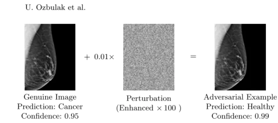
+ 0.01× = Genuine Image Prediction: Cancer Confidence: 0.95 Perturbation (Enhanced×100 ) Adversarial Example Prediction: Healthy Confidence: 0.99
Fig. 1.A genuine image, initially classified ascancer with 0.95 confidence by a deep learning model, is perturbed to become an adversarial example. This adversarial ex-ample is then classified ashealthywith 0.99 confidence by the same model.
labor with automation for a number of medical diagnosis tasks [6]. However, a recent development called adversarial examples showed that deep learning models are vulnerable to gradient-based attacks [12]. These so-called adversarial examples are now considered a major security flaw, since they allow for the use of possible fraud schemes (e.g., for insurance claims) when deep learning models are deployed for clinical tasks [6].
The study of adversarial examples started with [12], in which the authors observed that small pixel modifications led to large changes in the prediction. Ever since, numerous attempts were made to mitigate the impact of adversarial examples and to fix this so-called security flaw, only to be found ineffective by subsequent studies [3]. Although the effects of adversarial examples are largely studied for non-medical datasets, it was also shown that classification problems in medical imaging datasets are of no exception to this exploit [6]. An adversarial example in the context of breast cancer classification is given in Figure 1.
In the field of non-medical imaging, pixel by pixel detail is most of the time not task critical. As a result, segmentation problems are often expressed as de-tection or localization problems [5]. However, in medical imaging, precision is of utmost importance. Therefore, instead of detection or localization, segmentation covers a large portion of medical imaging problems [8].
Even though adversarial examples are studied extensively in the context of classification problems, it is only recently that studies started to investigate this phenomenon in the context of segmentation problems [1,13]. Thus far, in terms of segmentation, adversarial examples have been studied for the Pascal VOC [5] and Cityscapes [4] data sets, with a sole adversarial example generation method proposed in [13]. In particular, the Dense Adversary Generation (DAG) algorithm proposed in [13] aims to force deep learning models to segment all pixels wrong. Although the authors report that their algorithm is able to create adversarial examples in the context of segmentation, the resulting segmentation predictions, especially in the medical domain, are not realistic (i.e., the shape of
the prediction immediately gives away that the input has been tampered with, since the prediction shape is not specified).
In this study, we focus on analyzing adversarial examples in the context of medical image segmentation problems. We demonstrate that adversarial ex-amples indeed exist when dealing with medical image segmentation problems, discussing examples that have been obtained for glaucoma optic disc segmen-tation [10] and ISIC skin lesion segmensegmen-tation [7]. Furthermore, we introduce a novel algorithm that is tailored to produce targeted adversarial examples for image segmentation problems.
To the best of our knowledge, this is the first study that analyzes the impact of adversarial examples, not only in the context of medical imaging but also in the case where the nature of the prediction is binary. Additionally, our algorithm is the first approach towards producing targeted adversarial examples for image segmentation that leads to a convincing prediction shape of choice, thus exposing a large security threat for image segmentation models. Our algorithm, while achieving targeted predictions with a high success rate, modifies the original image so subtly that the modifications on the original image are, for the most part, invisible to the bare eye.
2
Notation and Framework
In this section, we explain the datasets, the deep learning models, the notation, and the evaluation metrics used throughout the paper.
Framework— In order to show the effectiveness of the proposed approach, we evaluate our attack on two datasets: the first one is the glaucoma optic disc segmentation dataset [10] and the second one is the ISIC skin lesion segmenta-tion dataset [7]. The results reported in Secsegmenta-tion 4 are obtained for two separate U-Net models which is one of the most used architectures in the field of medical segmentation [11]. These U-Net models have been trained on the two afore-mentioned datasets, achieving a segmentation effectiveness comparable to the state-of-the-art.
Neural Network Notation — We define the forward pass in a neural network as a function g with the weights and parameters of the same network detailed asθ. This function takes an input imageXof sizeC×H×W, withC, H, andW representing the number of channels (i.e., 1 for grayscale images, 3 for colored images), the height, and the width of the input image, respectively. In this setting, g(θ,X) represents the prediction of this neural network for a given input image X. The prediction is of size M ×H ×W, where M is the total number of classes (e.g., two in the case of binary segmentation). We defineY:= arg maxM(g(θ,X)) as the prediction of the neural network after discretization,
containing prediction classes (i.e., values from 0 toM−1) per pixel and having a size ofH×W.
Distance Metrics— When an adversarial example is generated, a distance metric is required in order to measure the difference between the original image and the generated image. Following previous studies [2], we use the Euclidian
dis-tance (L2) and the max distance (L∞), with the latter measuring the maximum
change for a single pixel among all pixels.
Accuracy Metrics— In order to quantify the accuracy of the adversarial example generation, we calculate the intersection over union (IoU) and the pixel accuracy (PA) between the target mask and the predicted segmentation mask associated with the adversarial example produced. In our settings where the background label is selected as 0, IoU and PA are defined as follows:
IoU(Y1,Y2) =X i,j Ai,j∩Bi,j .X i,j Bi,j, PA(Y1,Y2) = X i,j Ai,j . (H×W),
for (i, j)∈({1,· · · , H},{1,· · ·, W}) and whereAi,j =1{Y2
i,j=Y1i,j} andBi,j=
1{Y2
i,j+Y1i,j6=0}, with1representing the indicator function.
3
Generating Adversarial Examples
To justify our design choices, we briefly highlight the differences between clas-sification and segmentation in terms of adversarial example generation, before detailing our algorithm for generating adversarial examples for image segmenta-tion.
Adversarial Target — In classification, the adversarial target is often a single class [9]. However, in segmentation, the target is a mask. Thus, the aim is to change the prediction of not just one but of a large number of labels.
Perturbation Multiplier — In the case of classification (when a single class is targeted), the optimization is influenced by only one source. However, in segmentation, as a consequence of the adversarial target being a mask, the optimization is influenced by a large number of sources (i.e., individual pixels). As a result, the perturbation multiplier (i.e., the learning rate) is harder to tune. Keeping the aforementioned differences in mind and building upon the knowl-edge acquired from studying adversarial examples in classification problems, we propose the Adaptive Segmentation Mask Attack (ASMA), a novel algorithm for generating targeted adversarial examples for image segmentation models. 3.1 Adaptive Segmentation Mask Attack (ASMA)
As a starting point, we use the standard way of adversarial example generation, which is defined as follows:
minimize||X − (X+P)||2, such that arg max g(θ,(X+P))
=YA , (X+P)∈[0,1]C×H×W. This equation iteratively aims at finding a small perturbationPthat is suf-ficient to change the prediction of the model to YA, which we will refer to as
the target adversarial mask, while keeping theL2distance between the original imageXand its adversarial counterpartX+Pminimal. In this setting, a pertur-bation is calculated in an iterative manner, multiplied with a constant, and then
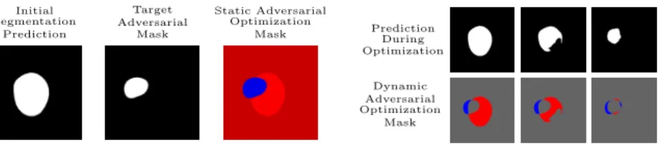
Initial Segmentation Prediction Target Adversarial Mask Static Adversarial Optimization
Mask PredictionDuring Optimization
Dynamic Adversarial Optimization
Mask
Fig. 2.An example adversarial optimization mask used by the static and the dynamic mask approaches, visualized in terms of the difference between the initial prediction and the targeted prediction.
added to the image: Xn+1 =Xn+αPn. We now detail how the perturbation
Pn is calculated.
Static Segmentation Mask (SSM) — In the context of adversariality, a targeted segmentation attack must (i) increase the prediction likelihood of the selected foreground pixels in the target adversarial mask (i.e., blue areas in the static adversarial optimization mask in Figure 2), while (ii) reducing the prediction likelihood of all other pixels that are not specified in the same mask (i.e., red areas in the static adversarial optimization mask in Figure 2). To achieve this property, we write Pn as a sum of perturbations as follows:
Pn = M−1 X c=0 ∇x g(θ,Xn)c 1{YA=c} , (1)
where denotes the Hadamard product and YA, again, denotes the desired prediction mask for the adversarial example that contains class labels (as shown in Figure 2).g(θ,X)c, on the other hand, denotes the channels of the prediction
made by the neural network (i.e., in the case of binary prediction, c = 0 for background channel andc= 1 for foreground channel).
We will now describe how we improve this approach.
Adaptive Segmentation Mask (ASM) — When the static mask ap-proach is used to generate adversarial examples, the gradient is sourced from the same number of target pixels in the target adversarial mask at each iter-ation. However, during the adversarial optimization, the prediction of certain pixels may already be correct (e.g., gray areas in the dynamic masks given in Figure 2), and may thus not require any further optimization. In order to ensure that the optimization is only sourced from pixels whose predictions are not in line with the target adversarial mask, we introduce an approach that makes use of adaptive mask targeting. To achieve this property, we writePn as follows:
Pn = M−1
X
c=0
∇x g(θ,Xn)c 1{YA=c} 1{arg maxM(g(θ,Xn))6=c}. (2)
Writing Pn this way ensures that the gradient is only sourced from pixels
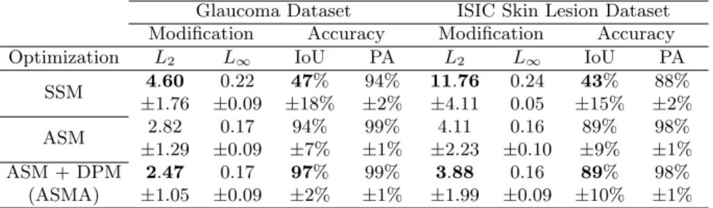
Table 1. Experimental results in terms of image modification and prediction mask accuracy. We highlight theL2distances and IoU overlaps to emphasize the increase in
the effectiveness of the optimization technique between the first and the last version. Note that numbers listed in this table are calculated for images whose pixel values are between 0 and 1.
Glaucoma Dataset ISIC Skin Lesion Dataset Modification Accuracy Modification Accuracy Optimization L2 L∞ IoU PA L2 L∞ IoU PA
SSM 4.60 0.22 47% 94% 11.76 0.24 43% 88% ±1.76 ±0.09 ±18% ±2% ±4.11 0.05 ±15% ±2% ASM 2.82 0.17 94% 99% 4.11 0.16 89% 98% ±1.29 ±0.09 ±7% ±1% ±2.23 ±0.10 ±9% ±1% ASM + DPM 2.47 0.17 97% 99% 3.88 0.16 89% 98% (ASMA) ±1.05 ±0.09 ±2% ±1% ±1.99 ±0.09 ±10% ±1%
Using the proposed adaptive segmentation mask approach, the number of pixels that source the optimization process starts high and as the prediction becomes in line with the target adversarial mask, lessens gradually.
Dynamic Perturbation Multiplier (DPM)— Since the usage of ASM progressively reduces the number of pixels the optimization sources from, setting the perturbation multiplierαto a fixed number either causes the optimization to halt whenαis low or causes it to create large perturbations when αis high. Therefore, we employ a dynamic perturbation multiplier strategy in our adaptive mask approach, usingαn=β×IoU(YA,Yn) +τ, whereβandτare parameters
used to calculate the final perturbation multiplier, also taking into account the IoU score of the prediction at thenth iteration. This method allows increasing the value of the multiplier dynamically as the number of pixels to be optimized decreases.
We name the adversarial example generation method that incorporates the aforementioned techniques (i.e., ASM and DPM) theAdaptive Segmentation Mask Attack (ASMA). Note our algorithm also works in the case where the prediction is not binary.
4
Experiments
Table 1 presents quantitative results on the viability of the proposed algorithm for adversarial example generation. Specifically, Table 1 shows the degree of per-turbation in terms of L2 and L∞ distances, as well as the mask accuracy of
the produced adversarial examples in terms of IoU and PA, hereby detailing the influence of the incremental updates (i.e., SSM, ASM, and DPM) that were discussed in Section 3.1. The values that can be found in Table 1 have been determined by calculating the mean and the standard deviation obtained from the optimization of 1000 adversarial examples. For each of those optimizations, the target adversarial mask is randomly selected among the masks of the other samples, so to have a realistic target in terms of medical image segmentation.
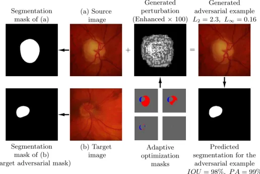
+ = Segmentation mask of (a) (a) Source image Generated perturbation (Enhanced×100) Generated adversarial example L2= 2.3, L∞= 0.16 Segmentation mask of (b) (Target adversarial mask)
(b) Target image Adaptive optimization masks Predicted segmentation for the
adversarial example
IOU = 98%, P A= 99%
Fig. 3. An example optimization of an adversarial example for segmentation using ASMA. Best viewed in color.
To find an optimal perturbation multiplier when DPM is not incorporated, we usedα∈ {1e−8,1e−7,1e−6, 1e−5}; when DPM is incorporated into the opti-mization, we useβ ∈ {1e−6,5e−6,1e−5} andτ = 1e−7. Results are listed for the experiment that achieves the highest average IoU score throughout the 1000 generated adversarial examples for the selected set of parameters.
As can be observed from Table 1, the proposed method, when all enhance-ments introduced in Section 3.1 are incorporated, achieves 97% and 89% IoU overlap with the target mask that was used for initiating the optimization, with L2 perturbations as low as 2.47 and 3.88 for the glaucoma optic disc and the ISIC skin lesion segmentation problems, respectively. For a more intuitive under-standing, anL2 perturbation of 3.88 corresponds to a modification of less than 1% of the images used in this study. Our experiments showed that, using ASMA, tuning the perturbation multiplier parametersβ andτ is not a difficult task, as we were able to achieve high IOU overlap with low L2 and L∞ perturbations
with only 3 possible combinations ofβ.
Apart from the quantitative results presented in Table 1, we also provide a qualitative overview of the approach used to generate adversarial examples in Figure 3. Specifically, Figure 3 shows the optimization procedure, a generated adversarial example, and the resulting predicted segmentation for a sample taken from the glaucoma optic disc dataset [10]. As can be seen, our algorithm is able
to completely change the prediction to the desired output mask (taken from another sample in the dataset) with an IoU success rate of 98%.
5
Conclusions and Future Work
In this paper, we demonstrated that deep learning-based models for medical im-age segmentation are vulnerable to attacks using adversarial examples, hereby focusing on skin lesion and glaucoma optic disc segmentation. Specifically, we in-troduced the Adaptive Mask Segmentation Attack, a novel algorithm that is able to produce adversarial examples with realistic prediction masks that have been altered to be misclassified, using perturbations mostly invisible to the human eye. The source code of our adversarial attack, as well as additional examples, can be found athttps://github.com/utkuozbulak/adaptive-segmentation-mask-attack. Although we were able to observe similar results on different models, as well as transferability of our generated adversarial examples to other models, we leave it to future work to perform a more detailed analysis and to examine corresponding novel defense mechanisms against attacks that leverage realistic prediction masks.
Acknowledgements
The research activities described in this paper were funded by Ghent University Global Campus, Ghent University, imec, Flanders Innovation & Entrepreneur-ship (VLAIO), the Fund for Scientific Research-Flanders (FWO-Flanders), and the EU.
References
1. Arnab, A., Miksik, O., Torr, P.H.: On the robustness of semantic segmentation models to adversarial attacks. In: Proceedings of the IEEE Conference on Com-puter Vision and Pattern Recognition. pp. 888–897 (2018)
2. Carlini, N., Wagner, D.A.: Towards evaluating the robustness of neural networks. CoRRabs/1608.04644(2016)
3. Carlini, N., Wagner, D.A.: Adversarial examples are not easily detected: Bypassing ten detection methods. CoRRabs/1705.07263(2017)
4. Cordts, M., Omran, M., Ramos, S., Rehfeld, T., Enzweiler, M., Benenson, R., Franke, U., Roth, S., Schiele, B.: The cityscapes dataset for semantic urban scene understanding. In: Proc. of the IEEE Conference on Computer Vision and Pattern Recognition (CVPR) (2016)
5. Everingham, M., Eslami, S.M.A., Van Gool, L., Williams, C.K.I., Winn, J., Zisser-man, A.: The pascal visual object classes challenge: A retrospective. International Journal of Computer Vision111(1), 98–136 (Jan 2015)
6. Finlayson, S.G., Kohane, I.S., Beam, A.L.: Adversarial attacks against medical deep learning systems. arXiv preprint arXiv:1804.05296 (2018)
7. Gutman, D., Codella, N.C.F., Celebi, M.E., Helba, B., Marchetti, M.A., Mishra, N.K., Halpern, A.: Skin lesion analysis toward melanoma detection: A challenge at the international symposium on biomedical imaging (ISBI) 2016, hosted by the international skin imaging collaboration (ISIC). CoRRabs/1605.01397(2016) 8. Heimann, T., Meinzer, H.P.: Statistical shape models for 3d medical image
seg-mentation: a review. Medical image analysis13(4), 543–563 (2009)
9. Kurakin, A., Goodfellow, I., Bengio, S.: Adversarial examples in the physical world. CoRRabs/1607.02533(2016)
10. Pena-Betancor, C., Gonzalez-Hernandez, M., Fumero-Batista, F., Sigut, J., Medina-Mesa, E., Alayon, S., de la Rosa, M.G.: Estimation of the relative amount of hemoglobin in the cup and neuroretinal rim using stereoscopic color fundus images. Investigative ophthalmology & visual science56(3), 1562–1568 (2015) 11. Ronneberger, O., Fischer, P., Brox, T.: U-net: Convolutional networks for
biomedi-cal image segmentation. In: Medibiomedi-cal Image Computing and Computer-Assisted In-tervention – MICCAI 2015. pp. 234–241. Springer International Publishing, Cham (2015)
12. Szegedy, C., Zaremba, W., Sutskever, I., Bruna, J., Erhan, D., Goodfellow, I., Fergus, R.: Intriguing properties of neural networks. CoRRabs/1312.6199(2013) 13. Xie, C., Wang, J., Zhang, Z., Zhou, Y., Xie, L., Yuille, A.: Adversarial examples for semantic segmentation and object detection. In: Proceedings of the IEEE In-ternational Conference on Computer Vision. pp. 1369–1378 (2017)