Learning sparse representation for image signals

(1)

c

(2)

LEARNING SPARSE REPRESENTATION FOR IMAGE SIGNALS

BY

ZHAOWEN WANG

DISSERTATION

Submitted in partial fulﬁllment of the requirements

for the degree of Doctor of Philosophy in Electrical and Computer Engineering in the Graduate College of the

University of Illinois at Urbana-Champaign, 2014

Urbana, Illinois

Doctoral Committee:

Professor Thomas S. Huang, Chair Professor Mark Hasegawa-Johnson Professor Zhi-Pei Liang

(3)

ABSTRACT

Natural images have the intrinsic property that they can be sparsely repre-sented as a linear combination of a very small number of atomic signals from a complete basis or an overcomplete dictionary. This sparse representation prior has been successfully exploited in a variety of image processing appli-cations, ranging from low level recovery to high level semantic inference. A good sparse representation is expected to have high ﬁdelity to the observed image content and at the same time reveal the underlying structure and semantic information. In this dissertation, we address the problem of how to learn such representation or dictionary from training images, particularly for the tasks of super-resolution, classiﬁcation, and opportunistic sensing.

Image super-resolution is an ill-posed problem in which we want to recover the high-resolution image from the corresponding low-resolution image. We formulate a coupled dictionary learning algorithm which explicitly learns the transform between the high and low-resolution feature spaces such that the sparse representation inferred from a low-resolution patch can faithfully reconstruct its high-resolution version. The resulting bilevel optimization problem is solved using a stochastic gradient descent method with the gra-dient of sparse code found by implicit diﬀerentiation. A feed-forward deep neural network motivated by this sparse coding model is designed to further improve the eﬃciency and accuracy.

The Sparse Representation-based Classiﬁcation (SRC) has been used in many recognition tasks with the dictionary consisting of training data from all classes. We design a more compact and discriminative dictionary for SRC using the “pulling” and “pushing” actions inspired from Learning Vector Quantization (LVQ). The learned dictionary is applied to hyper-spectral image classiﬁcation, with additional spatial neighborhood information in-corporated using a probabilistic formulation.

(4)

margin-based perspective into the classiﬁer. The decision boundary and classiﬁcation margin of SRC are analyzed in the local regions where the support of sparse code is stable. Based on the derived margin, we learn a discriminative dictionary with maximized margin between classes such that SRC can have better generalization capability.

Opportunistic sensing deals with actively recognizing an image object with restricted sensing resources. Just as in compressive sensing, we show that dynamically optimized sensing operations (including but not limited to linear projections) can yield better classiﬁcation results for signals with sparse structure. We develop a greedy sensing strategy using class entropy criteria, as well as a long-term policy learning method using the Partially Observable Markov Decision Process (POMDP) customized for heterogeneous resource constraints and discriminative classiﬁers.

The sensing, recovery and recognition tasks studied in this dissertation exemplify a closed loop of general image processing, and we demonstrate that in each processing step a dictionary or a sensing operation adapted to signals’ sparse characteristic can lead to remarkably improved performance.

(5)

(6)

ACKNOWLEDGMENTS

Foremost, I would like to express sincere gratitude to my adviser, Professor Thomas Huang, for sharing with me his expertise, vision and passion in research during my entire Ph.D. study, without which this dissertation would not have been possible.

I would also like to give my thanks to Dr. Nasser Nasrabadi, my mentor at ARL, for his guidance and support. It is a both productive and enjoyable experience to work with him. I am grateful to Professor Mark Hasegawa-Johnson and Professor Zhi-Pei Liang for serving on my doctoral committee and oﬀering invaluable comments and suggestions in the preparation of this dissertation.

Over the past ﬁve years, it has been my great honor to collaborate with many outstanding researchers including Ercan E. Kuruoglu at Italian Na-tional Council of Research, Jinjun Wang and Jing Xiao at Epson, and Jon Brandt, Hailin Jin and Zhe Lin at Adobe. Every one of them has helped sharpen my skills and broaden my perspective. There are also other fellow students and collaborators having directly or indirectly contributed to this dissertation: Jianchao Yang, Xi Zhou, Liangliang Cao, Zhen Li, Min-Hsuan Tsai, Jiangping Wang, Xinqi Chu, Kai-Hsiang Lin, Zhangyang Wang, Wei Han, Ning Xu, Yingzhen Yang, Shiyu Chang, Ding Liu, Po-Sen Huang, Mark Moll and Devin Grady, to all of whom I owe my sincere gratitude.

My thanks also go to many other friends, in particular to all the former and current members of the Image Formation and Processing (IFP) group whose continuing support and encouragement has made my Ph.D. career a memorable and valuable journey.

Lastly and most importantly, I want to thank my parents and my wife for their boundless love, understanding, and support in all the ways in my life.

(7)

CHAPTER 1 INTRODUCTION

Seeking meaningful representations for signals to capture their useful charac-teristics is one of the key problems studied in signal processing and pattern recognition. In the early days, people tended to represent signals in a “smooth” form, which motivates the techniques such as anisotropic ﬁltering [1] and total variation [2]. Representations with orthogonal bases were preva-lent due to their mathematical simplicity and computational eﬃciency. Well-known examples include wavelets for image compression [3] and denoising [4]. In recent years, more attention has been focused on representing a signalx

as the linear combination of a small number of atomic elements, called atoms, from a pre-deﬁned basis or overcomplete dictionary D with K atoms:

x=Dα, ∥α∥0 ≪K, (1.1)

where αis the sparse coeﬃcient vector, or sparse code, for x. ∥ · ∥0 denotes

the ℓ0_{-norm which is used to count the number of non-zero elements, or}

sparsity, in the sparse code α. Sparse representation assumes that, for any signal of our interest, its corresponding sparse code has a sparsity far less than the total number of atoms inD. By using an over-complete dictionary

D which has more elementary signal atoms than signal dimensions, we are able to parsimoniously describe a much wider range of signal phenomena [5]. To ﬁnd the sparsest α, we need to solve the following ℓ0 minimization problem:

min

α ∥α∥0, s.t.x=Dα. (1.2) Unfortunately, solving (1.2) requires intractable combinatorial optimization when the linear constraint is underdetermined. Approximate solutions can be found using greedy basis pursuit algorithms [6, 7], whose accuracy cannot be guaranteed. Alternatively, the ℓ1_{-norm is commonly used in place of}

(10)

compressive sensing theory [8, 9], is known to give the same solution under broad conditions for sparse enoughα. In many cases, the strict constraint of

x=Dα also needs to be relaxed to account for noise contamination, which results in the ℓ1_{-norm regularized minimization problem:}

min

α ∥x−Dα∥

2

2+λ∥α∥1, (1.3)

where λ>0 is a regularization parameter to balance between reconstruction error and sparsity.

The sparse coding based on Eq. (1.3) and its variants have been widely applied in image processing and computer vision problems including de-noising [10, 11], inpainting [12], super-resolution [13, 14], face recognition [15], motion segmentation [16, 17], action recognition [18], sensor fusion [19, 20], etc.. In almost all of these applications, using sparsity as a prior leads to state-of-the-art results [21]. The dictionary D plays an important role in the success of sparse representation. It is found that dictionaries learned from data [22, 23, 24, 25] and adapted to speciﬁc tasks [26, 27] can signiﬁcantly outperform analytically designed bases and conventional reconstruction-based dictionaries. However, how to learn a dictionary that induces sparse, robust and informative representations remains an unsolved problem in general.

In this dissertation, we explore learning good sparse representation in the context of three particular image applications: super-resolution, classiﬁcation and opportunistic sensing. We demonstrate that the entire pipeline of image processing (consisting of acquisition, recovery and understanding) can beneﬁt from learned representations.

Image Super-resolution Image super-resolution (SR) comprises tech-niques for estimating a high-resolution (HR) image from one or several cor-responding low-resolution (LR) images, in the hope of easing the resolution limitations of optical sensors. It has important applications in surveillance, remote sensing, consumer photo editing, image content retargeting, etc.. Since SR was ﬁrst formally investigated in the work of Tsai and Huang [28], various approaches have been proposed [29, 30, 31]. For the most challenging single image SR, machine learning approaches [32, 33, 34, 35] which learn the relationship between HR and LR images from training data prove to be more

(11)

promising than traditional methods based on signal reconstruction.

In single image SR, the unknown HR image x is related to the observed LR image y through a linear transform in the noise-free situation:

y=SHx, (1.4)

where S and H are downsampling and blurring operators, respectively. The linear system in (1.4) is heavily ill-posed and extra regularization is necessary to get a stable solution of x. Sparse representation eﬀectively oﬀers such a regularization as shown in [36, 13], where both xand y are sparely encoded according to (1.3) with respective to their individual dictionaries Dx and

Dy. The sparse code robustly inferred fromycan then be used to recoverx. Ideally, two dictionaries should satisfy the relationship Dy=SHDx so that any HR and LR image pair have the same sparse representation. However, the ﬁltersSandH are often unknown. Therefore, the dictionaries are learned in the joint space of x and y [36, 13], which is not consistent with the way they are used in recovery.

In this dissertation, a novel dictionary learning framework for coupled feature spaces is formulated such that we explicitly enforce the requirement that the sparse code evaluated for y can faithfully reconstructx using their respective dictionaries. Learning coupled dictionaries has many other poten-tial applications, e.g., texture transfer, compressive sensing. However, this problem has been little addressed in the literature. We also implement a deep neural network based on sparse coding approximation so that the eﬃciency and accuracy of sparse recovery are both improved.

Image Classification Although the primary goal of sparse representa-tion is for signal restorarepresenta-tion, it has also seen growing applicarepresenta-tion in image classiﬁcation. Face recognition [15], texture classiﬁcation [37] and objective categorization [38] are among the early successful examples.

The Sparse Representation-based Classiﬁcation (SRC) proposed in [15] is a pioneering work in this direction. In SRC, a signal xfrom class cis assumed to lie in or near a low-dimensional subspace spanned by the atoms in the class-speciﬁc dictionary Dc. If we try to represent x using the composite dictionary D=[D1, ...,DC] for all the C classes, the resulting sparse code

(12)

which is associated with its class.

Although SRC demonstrates good performance empirically, its working mechanism is obscure and a principled way to construct its dictionary is lacked. In the original work of [15], Dc consists of all the training samples from classc, which is not practical if the total class number or the training set is large. Traditional dictionary learning methods for sparse representation, such as Method of Optimal Direction (MOD) [39], K-SVD [40, 41], and the ℓ1-relaxed formulations [42, 43], all focus on minimizing signal reconstruction error and thus are not optimized for classification task. There are quite a few recent papers trying to learn dictionaries with more discriminative power by augmenting the reconstructive objective function in (1.3) with additional discrimination terms such as Fisher discriminant criterion [44], structural incoherence [25], class residual difference [45, 46] and mutual information [18]. Most of these discrimination metrics are heuristic and not geared to the mechanism of SRC. Sparse codes generated by discriminative dictionaries are also used as the input features of general classification models other than SRC [47, 24, 26].

Besides classifying each signal individually, SRC can also exploit the struc-ture among relevant signals for better performance. The joint sparse model has been used in multi-view recognition [19, 20] and spatial-spectral clas-siﬁcation in remote sensing [48, 49] for a more robust estimation of sparse code. The dictionaries used are usually not customized to enforce joint sparse representation.

A large portion of this dissertation is devoted to the learning of discrimina-tive dictionaries for SRC with application to both hyper-spectral and visual imageries. We generalize the idea of Learning Vector Quantization (LVQ) [50] to dictionary optimization for sparse signals, and also relate it to a maximum margin dictionary learning framework developed based on our in-depth analysis of SRC. Our proposed learning algorithm is favorable both theoretically and experimentally.

Opportunistic Sensing Sparse representation also enables eﬃcient sig-nal acquisition. In the well-known compressive sensing problem [8, 9], sparse prior has been used to recover signal from a small number of incoherent linear measurements. The problem requires solving an underdetermined linear systemy=M x, which is similar to the image SR problem in (1.4) but

(13)

with extra freedom to design the measurement matrix M. Conventionally a random matrixM is preferred due to theoretical guarantees of its incoherence with any sparsifying basis D. Lately, learning based algorithms have been proposed to optimize M either according to some analytical criteria derived from recovery conditions such as mutual coherence [51, 52, 53], or using data-driven approaches to minimize the empirical reconstruction error on training data [22, 26]. It has been found that simultaneous optimization of sensing matrix and signal representation leads to the best recovery performance [52]. On the other hand, adaptively designed measurement vectors in sequential compressive sensing can further improve reconstruction accuracy [54, 55, 56] or reduce the required number of samples [57].

In this dissertation, we consider the problem of opportunistic sensing under limited sensing resources with the goal of recognition instead of re-construction. As less information is usually needed in recognition than in reconstruction, even higher savings in sensing and computing resource is possible in opportunistic sensing than in compressive sensing, if the un-derlying signal representation is properly exploited. Moreover, perception based on information dynamically gleaned from a sparse set of simple yet complementary sensors is commonly employed in biological visual systems [58, 59, 60], which also inspires the paradigm of opportunistic sensing.

In our study of opportunistic sensing, we focus on designing sensing op-erations including both linear and non-linear ones, while recognizing the potential advantage of joint optimization over signal representation and ac-quisition. Acquiring linear measurements for the purpose of recognition is related to linear feature extraction and dimensionality reduction, which have been extensively explored in pattern recognition. Principle Component Anal-ysis (PCA), Linear Discriminant AnalAnal-ysis (LDA), and Canonical Correlation Analysis (CCA) are among the most classical methods. Methods based on graph embedding [61, 62, 63] have also been developed. Feature extraction approaches determine useful features during the oﬄine training stage, and therefore cannot take full advantage of the interactive sensing process by adapting to each signal individually.

When there is more than one sensor available, discrete sensor selection becomes another sensing operation. Sensor selection is also a well-studied problem, and has found its applications in wireless sensor network [64], target tracking [65], multimedia fusion [66], cognitive study [67], etc.. Most early

(14)

work on active sensor selection relies on a greedy strategy that selects the next best sensor based on some information theoretic criteria [68, 69]. To obtain a long-term optimal sensing strategy, Partially Observable Markov Decision Process (POMDP) which can consider an arbitrarily long time horizon has been used, with applications in gesture recognition [70], mine detection [71] and image object detection [72]. Information metric on the class posterior can be used to guide the policy learning in POMDP [73], and reinforcement learning algorithms are employed to learn object model and planning policy simultaneously [73, 72, 74].

In this dissertation, a unified framework is presented for dynamic sensor selection and linear feature extraction with the aim of classification. This framework is also extended to POMDP models, with extra considerations for heterogeneous resource constraints and discriminative classification models. The sparse prior of signals is exploited via a generative probabilistic model which is easily integrated with the evaluation of sensor informativeness. The proposed approaches are extensively evaluated in the tasks of multi-view/multi-modality/multi-feature vehicle classification and face recognition. The rest of this dissertation is organized as follows. We first introduce the coupled dictionary learning method for image SR in Chapter 2. Learning discriminative sparse representation for SRC is then discussed, with an LVQ inspired method presented in Chapter 3 for hyper-spectral images and a max-margin principle based method presented in Chapter 4 for general visual images. The problem of opportunistic sensing is explored in Chapter 5 for both greedy and long-term sensing strategies. Finally, Chapter 6 concludes with a summary and some future directions.

(15)

CHAPTER 2 COUPLED SPARSE CODING FOR SINGLE

IMAGE SUPER-RESOLUTION

2.1 Introduction

Image super-resolution (SR) comprises techniques for estimating a corre-sponding high-resolution (HR) image from one or several low-resolution (LR) images, which oﬀer the promise of partially overcoming inherent resolution limitations of low-cost imaging sensors (e.g., cell phone cameras or surveil-lance cameras), and allow better utilization of the growing capability of HR displays.

Conventional SR approaches usually require multiple LR input images of the same scene with sub-pixel translations. The SR task is thus cast as an inverse problem of recovering the underlying HR image by fusing the LR observed images, based on reasonable assumptions or prior knowledge about the observation model. Due to the irreversible high frequency information lost during the HR to LR degradation process, reconstructing a HR image is typically severely ill-conditioned. Various regularization techniques are therefore proposed to stabilize the solution of this ill-posed problem [29, 30, 31]. Unfortunately, the performance of these approaches is only acceptable for small upscaling factors (usually less than 2) [75].

More recently, example-based SR methods have been developed, which aim to learn the co-occurrence prior between HR and LR local patches from an external training database. The learned prior is employed to predict HR patches for unseen LR patches [32, 33, 76], and substantial improvement over the conventional methods has been achieved especially when only one or very few LR images are available. However, the example-based methods rely on a training database containing millions of HR/LR image patch pairs so that a generic image can be represented well, which makes the algorithms computationally intensive. Instead of relying on an external database, several

(16)

recently proposed approaches exploit the self-similarity properties of local image patches within and across diﬀerent spatial scales in the same image [77, 78, 34, 79, 35]. These approaches either need a separate deblurring process [77, 79], which is ill-posed and requires parameter tuning by itself, or place too much emphasis on local singular features, e.g., edges and corners, and thus yield unnatural-looking SR results [34, 35].

Motivated by the recent advances in compressive sensing [8, 80], which also focuses on solving an ill-posed linear inverse problem, Yang et al. in [36, 13] proposed to use sparse representation to recover HR images. Based on the assumption that the HR and LR image patches share the same sparse codes under their respective overcomplete bases (or dictionaries), they reconstructed HR patches with the sparse codes of corresponding LR patches and obtained both photo-realistic textures and sharp edges from a single input LR image. The HR and LR dictionary pair is crucial to the success of sparse representation-based SR approach, which essentially plays the role of an external database as in the case of example-based SR methods.

Learning overcomplete dictionaries from training data has attracted grow-ing interest from machine learngrow-ing and vision communities. A good dictio-nary is expected to be able to encode any signal of interest as the linear combination of a very small number of atoms from it, where the sparsity of coding coeﬃcients is usually enforced by an ℓ0 _or _ℓ1 _{penalty term. Many}

algorithms have been proposed to solve this learning problem; well-known examples include the ℓ0 _{sparsity constrained Method of Optimal Directions}

(MOD) [39] and K-SVD algorithm [40], an formulation with ℓ1 _sparsity

measure in [42], and an online large-scale learning algorithm in [43]. However, most prior works on dictionary learning only consider representing signals from a single space, which may not be suﬃcient in the problem of image SR where a pair of dictionaries should be jointly optimized to represent HR and LR signals respectively. In the original work of Yang et al. [13] who ﬁrst applied sparse representation to SR, the two feature spaces for HR and LR are concatenated together, and then the dictionary pair is trained together in their joint space as a single dictionary. As such, the resulting dictionaries are not indeed adapted to each of the feature spaces individually, and the resulting sparse codes for HR and LR patches are not guaranteed to be the same when they are evaluated from each single feature space.

(17)

which explicitly enforces that the sparse representation of an observed signal (the LR image) can well represent the sparse representation of its underlying latent signal (the HR image). The optimization employs a stochastic gradient descent procedure, where the gradient is computed via back-propagation and implicit diﬀerentiation. Dictionaries trained using our method lead to superior quality over dictionaries obtained by existing methods in single image SR both qualitatively and quantitatively. The sparse coding model is also extended to a feed-forward neural network [81] which further improves the SR performance by jointly optimizing over all the model parameters.

The remainder of this chapter is organized as follows. Section 2.2 reviews the sparse representation-based SR method and the conventional dictionary learning approaches. Our dictionary learning method for coupled feature spaces is presented in Section 2.3. In Section 2.4, we give the implementation details on single image SR with coupled dictionary learning, and show how to improve the algorithm eﬃciency without much compromise in performance. The extension to deep network implementation is discussed in Section 2.5. In Section 2.6, the eﬀectiveness of our approaches is demonstrated through comparisons with state-of-the-art image SR techniques as well as a human subjective evaluation. Conclusions are drawn in Section 2.7.

2.2 Related Work

Sparse representation has been widely applied to various low-level image processing tasks [40, 12], and it has been successfully introduced to single image SR in [13]. A LR image Y is commonly modeled as a blurred and downsampled version of its corresponding HR image X:

Y =SHX+ϵ, (2.1)

where S and H are downsampling and blurring operators, respectively, and

ϵ is a Gaussian noise. Solving X directly from (2.1) is a highly ill-posed problem. For SR, the unknown variables in X signiﬁcantly outnumber the known variables in Y, not to mention that we usually do not have precise knowledge about the linear operators S and H. Therefore, an additional

(18)

regularization is imposed on each local patch xin image X such that

x≈Dxα, for someα∈RK, ∥α∥0 ≪K, (2.2)

wherex∈Rd1 _{represents a HR image patch with its pixels stacked in a vector}

form, Dx ∈Rd1×K is the overcomplete dictionary for HR image patches with K>d1 basis atoms, andαis the sparse code forx. The sparsity prior imposed

by (2.2) is a common property of most natural images, and it serves as the cornerstone for SR reconstruction here.

Since the degradation model in (2.1) also applies to local patches, we can express the LR patch y corresponding to the HR patch xas follows:

y≈SHx≈SHDxα=Dyα, (2.3) where y∈ Rd2_{, and} _D

y =SHDx ∈Rd2×K is the dictionary for LR patches. Therefore, the same sparse code α can be used to represent both x and y

with respect to the dictionaries Dx andDy, respectively. Note that since we do not know the operators S and H, both Dx and Dy are to be learned.

Now suppose the dictionariesDx andDy are given; for an input LR patch

y, what we need is just to find the sparse code α for y, and reconstruct its HR patch as ˆx=Dxα. According to the compressive sensing theories [8, 9], if the sparse code α is sufficiently sparse, it can be efficiently recovered by solving the following ℓ1 regularized minimization problem:

min

α ∥y−Dyα∥

2

2+λ∥α∥1, (2.4)

where λ >0 is a regularization parameter. Once all the HR patches{x} are obtained, the entire HR image X can be reconstructed by placing them at appropriate locations.

In the following, we introduce two related dictionary learning techniques to obtain Dx and Dy, i.e., sparse coding in a single feature space and joint sparse coding in coupled feature spaces.

(19)

2.2.1 Sparse Coding

The goal of sparse coding is to represent an input signal x ∈ Rd approxi-mately as a weighted linear combination of a few basis atoms, often chosen from an over-complete dictionary D ∈ Rd×K (d < K). Sparse coding is the method to learn such a good set of basis atoms. Concretely, given the training data{xi}N_i₌₁, the problem of learning a dictionary for sparse coding, in its most popular form, is solved by minimizing the energy function that combines squared reconstruction errors and the ℓ1_{-sparsity penalties on the}

representations: min D,{αi}N i=1 N ∑ i=1 ∥xi−Dαi∥22+λ∥αi∥1 s.t. ∥D(:, k)∥2 ≤1, ∀k ∈ {1,2, ..., K}, (2.5)

where D(:, k) is the k-th column of D, αi is the sparse code of xi, and λ is a parameter controlling the sparsity penalty and representation ﬁdelity. The above optimization problem is convex in either Dor{αi}N

i=1 when the other

is ﬁxed, but not in both. When Dis ﬁxed, inference for {αi}Ni=1 is known as

the Lasso problem in the statistics literature; when{αi}N

i=1 are ﬁxed, solving

D becomes a standard quadratically constrained quadratic programming (QCQP) problem. A practical solution to (2.5) is to alternatively optimize over D and {αi}N_i₌₁, and the algorithm is guaranteed to converge to a local minimum [42].

2.2.2 Joint Sparse Coding

Unlike the standard sparse coding, joint sparse coding considers the problem of learning two dictionaries Dx and Dy for two coupled feature spaces with training pairs{xi,yi}iN=1. It is required that the paired samplesxi andyi can be represented as the sparse linear combinations of atoms from their respec-tive dictionariesDx and Dy using thesame sparse code αi. In this way, the relationship between the two feature spaces is encoded in the corresponding atoms in the two dictionaries. Yang et al. [13] addressed this problem by

(20)

generalizing the basic sparse coding scheme as follows: min Dx,Dy,{αi}N_i₌₁ N ∑ i=1 ( ∥xi−Dxαi∥22+∥yi−Dyαi∥22 ) +λ∥αi∥1, s.t. ∥Dx(:, k)∥2 ≤1, ∥Dy(:, k)∥2 ≤1. (2.6)

The formulation above basically requires that the resulting common sparse code αi should reconstruct both yi and xi well. Grouping the two recon-struction error terms together and denoting

¯ xi = [ xi yi ] , D¯ = [ Dx Dy ] , (2.7)

we can convert Eq. (2.6) to a standard sparse coding problem in the concate-nated feature space:

min ¯ D,{αi}N i=1 N ∑ i=1 ∥x¯i−Dα¯ i∥22 +λ∥αi∥1 s.t. ∥D(:, k)¯ ∥2 ≤1. (2.8)

Therefore, such a joint sparse coding scheme can only be claimed to be optimal in the concatenated feature space, but not in each feature space individually.

In testing, given an observed signaly, we want to recover the corresponding latent signal x by inferring their common sparse code α. However, since x

is unknown, there is no way to ﬁnd α in the concatenated feature space as has been done in training. Instead, we can only infer the sparse code of y

in its own feature space with respect to Dy, and use it as an approximation to the joint sparse representation forx andy, which is not guaranteed to be consistent with the sparse code of x with respect to Dx. Consequently, the accuracy of recovering xmay be undermined using the above jointly learned dictionaries.

(21)

2.3 Coupled Dictionary Learning for Sparse Recovery

In this section, we develop a dictionary learning method for coupled feature spaces such that the sparse representation of a signal in one feature space is optimized to well reconstruct its corresponding signal in the other space.

2.3.1 Problem Statement

Suppose we have two coupled feature spaces: the latent space X ⊆ Rd1

and the observable space Y ⊆ Rd2_{, where the signals are sparse,} _i.e._{, the}

signals have sparse representations in terms of certain dictionaries. Signals in Y are observable, and signals in X are what we want to recover or infer. There exists some mapping function F :X → Y (not necessarily linear and probably unknown) that maps a signal x inX to its corresponding signal y

in Y: y = F(x). We assume that the mapping function is nearly injective; otherwise, the inference for X fromY would be impossible. Our problem is to ﬁnd a coupled dictionary pair Dx andDy for spaceX andY respectively, such that given any signal y ∈ Y, we can use its sparse representation in terms of Dy to recover the corresponding latent signal x ∈ X in terms of

Dx. Formally, an ideal pair of coupled dictionariesDxandDy should satisfy the following equations for any coupled signal pair {xi,yi}:

zi = arg min αi ∥yi−Dyαi∥22 +λ∥αi∥1,∀i= 1...N (2.9) zi = arg min αi ∥ xi−Dxαi∥22 ,∀i= 1...N1 (2.10) where {xi} N

i=1 are the training samples from X, {yi}

N

i=1 are the training

samples fromY withyi =F(xi), and{zi} N

i=1 are the sparse representations.

Signal recovery from coupled spaces can be thought as a problem similar to compressive sensing [8, 80]. In the context of compressive sensing, the observation and latent spaces are related through a linear random projection function F. Dictionary Dx is usually chosen to be a mathematically deﬁned basis (e.g., wavelets), and Dy is obtained directly from Dx with the linear mapping F. Under some moderate conditions, the sparse representation

1_{Alternatively, one can require that the sparse representation of} _x

i in terms of Dx

is zi. However, since only the recovery accuracy of xi is concerned, we directly impose

(22)

of y derived from Eq. (2.9) can be used to recover x with performance guarantees. However, in more general scenarios where the mapping function F is unknown and may take a non-linear form2_{, the results of compressive}

sensing theory do not hold in general. Then it becomes more favorable to learn the coupled dictionaries from the training data using machine learning techniques.

2.3.2 Formulation

Given an input signal y, the recovery of its latent signal x consists of two sequential steps: first to find the sparse representationz of yin terms of Dy according to Eq. (2.9), and then to estimate the latent signal as ˆx = Dxz. Since the goal of our dictionary learning is to minimize the recovery error of ∥x−xˆ∥2₂, we define the following squared loss term:

L(Dx,Dy,x,y) = 1

2∥x−Dxz∥

2

2. (2.11)

Then the optimal dictionary pair {D∗_x,D_y∗} is found by minimizing the empirical expectation of (2.11) over the training signal pairs,

min Dx,Dy 1 N N ∑ i=1 L(Dx,Dy,xi,yi) s.t. zi = arg min α ∥yi−Dyα∥ 2 2+λ∥α∥1, for i= 1,2, ..., N, ∥Dx(:, k)∥2 ≤1, ∥Dy(:, k)∥2 ≤1, for k = 1,2, ..., K. (2.12)

Simply minimizing the above empirical loss does not guarantee that y can be well represented by Dy. Therefore, we can add one more reconstruction term to the loss function to ensure good representation of y,

L(Dx,Dy,xi,yi) = 1 2 ( γ∥xi−Dxzi∥22+ (1−γ)∥yi−Dyzi∥22 ) , (2.13) where γ (0< γ≤1) balances the two reconstruction errors.

2_{In the example of patch-based SR, the image degradation process} _F _{from HR space}

to LR space is no longer a simple linear transformation of blurring and downsampling if the signals in the LR space are represented as high frequency features of raw patches, which is typically employed for better visual eﬀect. We will discuss this in more detail in Section 2.4.

(23)

The objective function in (2.12) is highly nonlinear and nonconvex. We propose to minimize it by alternatively optimizing over Dx and Dy while keeping the other ﬁxed. When Dy is ﬁxed, the sparse representation zi can be determined for each yi with Dy, and the problem in (2.12) reduces to

min Dx N ∑ i=1 1 2∥Dxzi−xi∥ 2 2 s.t. zi = arg min α ∥yi−Dyα∥ 2 2+λ∥α∥1, for i= 1,2, ..., N, ∥Dx(:, k)∥2 ≤1, for k = 1,2, ..., K, (2.14)

which is a quadratically constrained quadratic programing that can be solved eﬃciently using conjugate gradient descent [42]. When Dx is ﬁxed, the optimization over Dy is more complicated and is discussed in the following.

2.3.3 Optimization for Dictionary

D

y

Minimizing the loss function of Eq. (2.12) over Dy is a highly nonconvex bilevel programming problem [82]. The upper-level optimization of (2.12) depends on the variable zi, which is the optimum of the lower-level ℓ1 -minimization. To solve this bilevel problem, we employ the same descent method developed in [38], which basically ﬁnds a descending direction along which the objective function will decrease smoothly with a small step. For easy of presentation, we drop the subscripts of xi,yi, andzi in the following. Applying the chain rule, we can evaluate the descending direction as

∂L ∂Dy = 1 2 ( ∑ j∈Ω ∂(γRx+ (1−γ)Ry) ∂zj dzj dDy + (1−γ)∂Ry ∂Dy ) , (2.15)

where we denote Rx = ∥Dxz −x∥22 and Ry = ∥Dyz −y∥22 as the

recon-struction residuals with representation z for x and y, respectively. zj is the j-th element ofz, and Ω denotes the index set for j such that the derivative dzj/dDy is well deﬁned. Let ˜z denote the vector built with the elements {zj}j∈Ω, and ˜Dx and ˜Dy denote the dictionaries that consist of the columns

(24)

in Dx and Dy associated with indices in Ω. It is easy to ﬁnd that ∂Rx ∂z˜ = 2 ˜D T x(Dxz−x), ∂Ry ∂z˜ = 2 ˜D T y(Dyz−y), ∂Ry ∂Dy = 2(Dyz−y)zT. (2.16)

To evaluate the gradient in Eq. (2.15), we still need to ﬁnd the index set Ω and the derivative dz˜/dDy. However, there is no analytical link between ˜z and Dy. We use the technique developed in [38] to ﬁnd the derivative in the following.

2.3.4 Sparse Derivative

For the Lasso problem in Eq. (2.9), we have the following condition for the optimal z [83]:

∂∥y−Dyz∥22

∂zj +λ sign(zj) = 0, ∀zj ̸= 0. (2.17) Accordingly, deﬁne our index set as Ω = {j|zj ̸= 0}, and we have

∂∥y−D˜yz˜∥22 ∂zj +λ sign(zj) = 0, ∀j ∈Ω, (2.18) or ˜ Dy T _˜ Dyz˜−D˜y T y+λsign( ˜z) = 0. (2.19) It is easy to show that ˜z is a continuous function of Dy [84]. Therefore, a small perturbation in Dy will not change the signs of the elements in ˜z. As a result, we can apply the implicit diﬀerentiation on Eq. (2.19) to obtain

∂{D˜y T _˜ Dyz˜−D˜y T y} ∂D˜y = ∂{−λ·sign( ˜z)} ∂D˜y ⇒ ∂D˜y T _˜ Dy ∂D˜y ˜ z+ ˜Dy T _˜ Dy ∂z˜ ∂D˜y − ∂D˜y T y ∂D˜y = 0. (2.20)

(25)

Then, we calculate the derivative as ∂z˜ ∂D˜y = ( ˜ Dy T _˜ Dy )₋1(_∂_D˜_yT_y ∂D˜y −∂D˜y T _˜ Dy ∂D˜y ˜ z ) , (2.21)

where we assume the solution to Eq. (2.9) is unique and ( ˜Dy T _˜

Dy)−1 exists. (2.21) only gives us the derivative of ˜zwith respect to ˜Dy, which is associated the index set Ω. The other derivative elements of∂zj/∂Dy required in (2.15) are simply set to zero, because it can be shown that the set Ω and the signs of ˜z will not change for a small perturbation in Dy as long as λ is not a transition point of y in terms of Dy [85]. As the chance for λ to be a transition point of y is low for any general distribution of y, (2.15) can approximate the true gradient in expectation. A more rigid treatment of this issue has been provided by Mairalet al. [26] which leads to an identical way to calculate the sparse code derivative.

2.3.5 Algorithm Summarization

With the gradient calculated as in (2.15), we employ a projected stochastic gradient descent procedure for the optimization of Dy due to its fast conver-gence and good behavior in practice. Because of the high nonconvexity of the bilevel optimization over Dy as well as the greedy nature of the alternative optimization overDxandDy, we can only expect to ﬁnd a local minimum for the learned coupled dictionaries, which is nevertheless suﬃcient for practical use as demonstrated in the experiments.

Algorithm 2.1 summarizes the complete procedures for our coupled dictio-nary learning algorithm. Some explanation are provided below:

• Line 2: Dx and Dy can be initialized in various ways, e.g., using the joint sparse coding in Section 2.2 or other standard sparse coding methods.

• Line 6: η(t) is the step size for stochastic gradient descent, which shrinks in the rate of 1/t.

• Line 7: To satisfy the dictionary norm constraint, we normalize each column of Dy to unitℓ2-norm.

(26)

Algorithm 2.1 Coupled Dictionary Training

1: input: training patch pairs{(xi,yi)}N_i₌₁, and dictionary sizeK. 2: initial: initialize D(0)x and D

(0)

y ,n = 0, t= 1. 3: repeat

4: for i= 1,2, ..., N do

5: Compute gradient a = dL(D(xn),Dy(n),xi,yi)/dDy according to (2.15);

6: Update Dy(n)=Dy(n)−η(t)·a;

7: Project the columns of D(yn) onto the unit ball; 8: t =t+ 1;

9: end for

10: UpdateDy(n+1) =D(yn);

11: UpdateDx(n+1) according to (2.14) with Dy(n+1); 12: n=n+ 1;

13: until convergence

14: output: coupled dictionaries D(xn) and D(yn).

The proposed coupled learning algorithm is generic, and hence can be potentially applied to many signal recovery and computer vision tasks, e.g., image compression, texture transfer. In the following, we will focus on its application to patch-based single image SR.

2.4 Image Super-resolution via Sparse Recovery

In this section, we discuss single image SR via sparse recovery, where the LR image patches constitute an observable space Y and the HR image patches constitute a latent space X. Coupled dictionary learning is applied to model the mapping between the two spaces, and the learned dictionaries are used to recover HR patch x for any given LR patch y.

2.4.1 Feature Extraction for SR

Instead of directly working on raw pixel values, we extract simple features from HR/LR patches respectively as the signals in their coupled spaces. The DC component is ﬁrst removed from each HR/LR patch because the mean value of a patch is always preserved well through the mapping from HR space to LR space. Also, we extract gradient features from the

(27)

bicubic-interpolated LR image patches as in Yang et al. [13], since the median frequency band in LR patches is believed to be more relevant to the missing high frequency information. Finally, all the HR/LR patch signals (extracted features) are normalized to unit length so that we do not need to worry about the shrinkage eﬀect of ℓ1_{-norm minimization on the sparse representations.}

As can be seen, the resultant HR/LR image patch (feature) pairs are tied by a mapping function far more complex than the linear system considered in most conventional inverse problems such as compressive sensing.

To train the coupled dictionaries, we sample a large number of training HR/LR image patch pairs from an external database containing clean HR images {Xi}n

i=1. Each HR image Xi is blurred, down-sampled and then interpolated using bicubic function to generate the corresponding LR image

Yi with the same size asXi. From these image pairs {Xi,Yi}ni=1, we sample

N pairs of HR/LR patches of sizep×p, and extract the patch features using the aforementioned procedures to obtain training data{(xi,yi)}Ni=1. To avoid

sampling too many smooth patches which are less informative, we eliminate those patches with small variances. Once the training data are prepared, the coupled dictionaries Dx and Dy can be trained.

2.4.2 Patch-wise Sparse Recovery

In the testing phase, we basically perform the same patch-wise sparse SR recovery as outlined in Section 2.2, but with the coupled dictionaries learned using Algorithm 2.1. The input LR imageY is ﬁrst interpolated to the size of the desired HR image, and then divided into a set of overlapping LR patches of size p×p. For each LR image patch, we extract its feature y as in the training phase, and compute its sparse code z with respect to the learned dictionary Dy. z is then used to predict the underlying HR image patch as

x=Dxz, with the DC component and norm adjusted according to the input LR patch. The predicted HR patches are tiled together to reconstruct the HR image X, where the average is taken for pixels in the overlapping region with multiple predictions. Algorithm 2.2 describes the sparse recovery SR method in detail.

Since the magnitude information of a signal is lost in its sparse recovery (typically∥Dxz∥2 <∥x∥2), extra consideration is given when we recover the

(28)

Algorithm 2.2 Super-Resolution via Sparse Recovery 1: input: coupled dictionaries Dx and Dy, LR image Y.

2: initialize: set HR image X =0; upscale Y by bicubic interpolation. 3: for each p×ppatch yp in Y do

4: setm= mean(yp),r =∥yp−m∥2;

5: extract gradient featurey from the normalized patch (yp−m)/r; 6: ﬁnd sparse codez = arg minα 1₂∥Dyα−y∥22+λ∥α∥1;

7: recover HR patch feature x=Dxz;

8: recover HR image patch xp = (c×r)·x/∥x∥2+m;

9: add xp to the corresponding pixels in X; 10: end for

11: average multiple predictions on overlapping pixels of X; 12: output: HR image X.

norm of HR image patches. From the raw training patches, we observe that the norm of a zero-mean HR image patch is approximately proportional to the norm of its zero-mean interpolated LR image patch. The proportional factor c(in the line 8 of Algorithm 2.2) is a constant greater than 1,3 _{depending on}

the SR upscaling factor. E.g., c = 1.2 is found by linear regression for the upscaling factor of 2.

2.4.3 Eﬃciency Improvements

The patch-wise sparse recovery approach can produce SR images of superior quality. However, the high computational cost associated with this approach has limited its practical use in real applications. To produce one SR image of moderate size, we need to process thousands of patches, each of which involves solving an ℓ1-regularized minimization problem. Therefore, reduc-ing the number of patches to process and findreduc-ing a fast solver for the ℓ1 minimization problem are the two directions for efficiency improvement. In the following, we briefly discuss a selective patch processing strategy and a feed-forward sparse coding approximation model that can significantly speed up our algorithm without much compromise on SR performance.

Natural images typically contain large smooth regions as well as strong discontinuities, such as edges and corners. Although simple interpolation methods for image upscaling, e.g., bilinear and bicubic interpolation, will

3_{HR image patches have better contrast, and consequently have larger magnitudes}

(29)

Figure 2.1: Comparison of RMSE in SR reconstruction between sparse recovery and bicubic interpolation. Sparse recovery performs better in regions indicated by red color; bicubic interpolation performs better in regions indicated by blue color; the two perform similarly in the remaining regions shaded in dark.

result in noticeable artifacts in regions with texture and edges, they perform reasonably well on smooth regions. This is supported by the observation from Fig. 2.1, where we upscale (by factor of 2) each patch in the “Lena” image using both bicubic interpolation and sparse recovery, and compare their respective Root Mean Square Error (RMSE). The red color indicates regions where our sparse recovery outperforms the bicubic interpolation in terms of RMSE; the blue color indicates regions where bicubic interpolation is better; and the two methods are comparable in the regions shaded in dark. From this ﬁgure, we can conclude: 1) the overall performance of the sparse recovery algorithm is better than the bicubic interpolation in most cases; 2) sparse recovery performs much better than bicubic interpolation in regions with edges and rich textures; and 3) sparse recovery and bicubic interpolation are comparable on large smooth regions. This observation suggests that we can selectively process those highly textured regions using the computationally more expensive sparse recovery technique, and apply the more economical bicubic interpolation for the remaining smooth regions. Here, we identify regions with edges and textures by simply measuring the variance of each image patch: if the variance of an image patch exceeds a threshold, we process it using sparse recovery; otherwise, bicubic interpolation is applied to estimate the HR image patch.

Another way to accelerate the sparse recovery method is to use an eﬃcient algorithm to ﬁnd the sparse codes which otherwise have to be solved from

(30)

the ℓ1 _{minimization problem. Several recent works have proposed to ﬁnd}

the fast approximation of the sparse code by learning feed-forward neural network models [86, 87, 81]. Given examples of input vectors paired with the corresponding optimal sparse codes (obtained by conventional optimization methods), these neural network models try to learn an efficient parameterized non-linear encoder function to predict the optimal sparse codes. In this work, we employ the network structure proposed in [81] to efficiently find the sparse codes for LR image patches.

2.5 From Sparse Coding to Deep Network

Neural networks can not only speed up the computation of sparse coding, but also provide a new framework for optimizing all the SR processing steps from end to end with deep architectures. Deep networks have been used for image SR in [88, 89] and achieved impressive improvements. However, it is not clear what kind of priors these deep networks have learned and enforced on HR images, since their structures are designed in a more or less intuitive way and have no correspondence to other shallow models.

In this section, we introduce a recurrent neural network (RNN), which closely mimics the behavior of sparse coding and at the same time beneﬁts from end-to-end optimization over training data. We demonstrate through this novel network that a good model structure capturing correct image prior still plays a crucial role in regularizing SR solution even when we have suﬃcient modeling capacity and training data.

2.5.1 LISTA Network for Sparse Coding

One key building block in our RNN model is based on the work in [81], where a Learned Iterative Shrinkage and Thresholding Algorithm (LISTA) is used to learn a feed-forward network to eﬃciently approximate sparse coding. As illustrated in Fig. 2.2, the LISTA network takes signal y as its input and outputs the sparse code α as it would be obtained by solving (2.9) for a given dictionary Dy. The network has a ﬁnite number of recurrent stages,

(31)

ߠ

ܵ

+

ܵ

+

ߠ

ܹ

ݕ

ߙ

ݖ

_ଵ

ݖ

_ଶ

Figure 2.2: A LISTA network [81] with 2 time-unfolded recurrent stages, whose output αis an approximation of the sparse code of input signaly. The linear weights W, S and the shrinkage thresholds θ are learned from data.

each of which updates the intermediate sparse code according to

zk+1 =hθ(W y+Szk), (2.22) where hθ is an element-wise shrinkage function deﬁned as

[hθ(a)]i = sign(ai)(|ai| −θi)+. (2.23)

Different from the iterative shrinkage and thresholding algorithm (ISTA) [90, 91] which finds an analytical relationship between network parameters (weightsW, S and thresholdsθ) and sparse coding parameters (Dy andλ), the authors of [81] learn all the network parameters from training data using a back-propagation algorithm called learned ISTA (LISTA). In this way, a good approximation of the underlying sparse code can be obtained after a fixed small number of recurrent stages.

2.5.2 Recurrent Network for Image SR

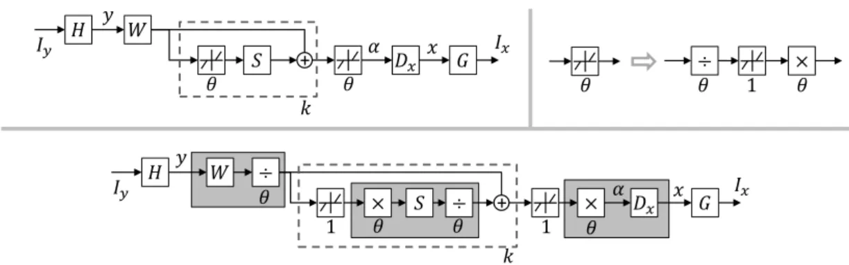
Given the fact that sparse coding can be eﬀectively implemented with a LISTA network, it is straightforward to formulate our RNN model that strictly mimics the processing ﬂow of the sparse coding based SR method [13] with multiple layers of neural networks. Same as most patch-based SR methods, our network takes the bicubic-upscaled LR image Iy as input, and outputs the full HR image Ix. Fig. 2.3 shows the main network structure, and each of the layers is described in the following.

The input image Iy ﬁrst goes through a convolutional layer H which extracts feature for each LR patch. There are my ﬁlters of spatial size sy×sy in this layer, so that our input patch size is sy×sy and its feature

(32)

ߠ ܵ + ܦ௫ ߠ ܹ ݕ ݔ ߙ ܪ ܫ௬ _ܩ ܫ௫ ݇ ߠ ߠ ൈ ൊ ߠ ͳ ͳ ܵ + ܦ௫ ͳ ܹ ݕ ݔ ߙ ܪ ܫ௬ ܫ௫ ܩ ݇ ߠ ൊ ൈ ߠ ൊߠ ൈߠ

Figure 2.3: Top left: the proposed RNN network with a patch extraction layer H, a LISTA sub-network for sparse coding (withk recurrent stages denoted by the dashed box), a HR patch recovery layer Dx, and a patch combination layer G. Top right: a neuron with adjustable threshold decomposed into two linear scaling layers and a unit-threshold neuron. Bottom: our RNN network re-organized with unit-threshold neurons and adjacent linear layers merged together in the gray boxes.

representation y has dimension my.

Each LR patchyis then fed into a LISTA network with krecurrent stages to obtain its sparse codeα∈Rn. Each stage of LISTA consists of two linear layers parameterized byW ∈Rn×my _and _S ∈Rn×n_{, and a nonlinear neuron}

layer with activation function hθ. The activation thresholds θ∈Rn are also to be updated during training, which complicates the learning algorithm. To restrict all the tunable parameters in our linear layers, we do a simple trick to rewrite the activation function as

[hθ(a)]i = sign(ai)θi(|ai|/θi−1)+ =θih1(ai/θi). (2.24) Eq. (2.24) indicates the original neuron with adjustable threshold can be decomposed into two linear scaling layers and a unit-threshold neuron, as shown in the top-right of Fig. 2.3. The weights of the two scaling layers are diagonal matrices deﬁned by θ and its element-wise reciprocal, respectively. The sparse code α is then multiplied with HR dictionaryDx ∈Rmx×n in the next linear layer, reconstructing HR patch xof size sx×sx =mx.

In the final layer G, all the recovered patches are put back to the corre-sponding positions in the HR image Ix. This is realized via a convolutional filter ofmxchannels with spatial sizesg×sg. The sizesg is determined as the number of neighboring patches that overlap with a center HR patch in each spatial direction. The filter will assign appropriate weights to the overlapped

(33)

pixels recovered from diﬀerent patches and take their weighted average as the ﬁnal prediction in Ix.

As illustrated in the bottom of Fig. 2.3, after some simple reorganizations of the layer connections, the network described above has some adjacent linear layers which can be merged into a single layer. This helps to reduce the computation load as well as redundant parameters in the network. The layers H and G are not merged because we apply additional nonlinear normalization operations on patches y and x, which will be detailed in Section 2.6.

Thus, there are totally 5 trainable layers in our network: 2 convolutional layers H and G, and 3 linear layers shown as gray boxes in Fig. 2.3. The k recurrent layers share the same weights and are therefore conceptually regarded as one. Note that all the linear layers are actually implemented as convolutional layers applied on each patch with ﬁlter spatial size of 1×1. Also note that all these layers only have weights but no biases (zero biases). Mean square error (MSE) is employed as the cost function to train the network, and our optimization objective can be expressed as

min

Θ ∑

i

∥RN N(I_y(i);Θ)−I_x(i)∥2₂, (2.25)

whereIy(i)andIx(i)are thei-th pair of LR/HR training data, andRN N(Iy;Θ) denotes the HR image for Iy predicted using the RNN model with param-eter set Θ. All the parameters are optimized through the standard back-propagation algorithm. Although it is possible to use other cost terms that are more correlated with human visual perception than MSE, our experimen-tal results show that simply minimizing MSE also leads to improvement in subjective quality.

2.5.3 Network Cascade for Scalable SR

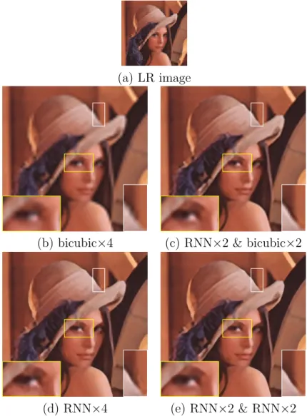
Like most SR models learned from external training examples, the RNN discussed previously can only generate HR images for a fixed upscaling ratio. A different model needs to be trained for each scaling factor to achieve the best performance, which limits the flexibility and scalability in practical use. One way to overcome this difficulty is to repeatedly enlarge the image by a

(34)

(a) LR image

(b) bicubic×4 (c) RNN×2 & bicubic×2

(d) RNN×4 (e) RNN×2 & RNN×2

Figure 2.4: SR results for Lena image upscaled by 4 times. (a) → (b) → (d) represents the processing flow with a single RNN×4 model. (a) → (c) → (e) represents the processing flow with two cascaded RNN×2 models. fixed scale until the resulting HR image reaches a desired size. This practice is commonly adopted in the self-similarity based methods [34, 35, 89], but is not so popular in other cases for the fear of error accumulation during repetitive upscaling.

In our case, however, it is observed that a cascade of RNNs (CRNN) trained for small scaling factors can generate even better SR results than a single RNN trained for a large scaling factor, especially when the target upscaling factor is large (greater than 2). The example shown in Fig. 2.4 tells part of the underlying reason. Here an input image (a) is magniﬁed by×4 times using a single RNN×4 model (d), as well as using a cascade of two RNN×2 models

(35)

RNN₁ bicubic ܫ଴ _RNN 2 bicubic ܫመଵ ܫመଶ ܫଵ MSE ܫ_ଶ MSE

scale ൈ1 scale ൈ ݏ scale ൈ ݏଶ

Figure 2.5: Training cascade of RNNs with multi-scale objectives. (e). It can be seen that the cascaded network generates a more natural-looking image for the complex object structures in the enlarged regions, while the single network produces notable artifacts. By further comparing the bicubic input to the single RNN×4 (b) with the input to the second cascaded RNN×2 (c), we ﬁnd the latter one is much shaper and has much fewer artifacts along the edges. This indicates that (c) contains more relevant information but less noise than (b), and therefore it is easier to restore the HR image from (c) than from (b).

To get a better understanding of the above observation, we can draw a loose analogy between the SR process and a communication system. Bicubic interpolation is like a noisy channel through which an image is “transmitted” from LR domain to HR domain. And our RNN model (or any SR algorithm) behaves as a receiver which recovers clean signal from noisy observation. A CRNN is then like a set of relay stations that enhance signal-to-noise ratio before the signal becomes too weak for further transmission. Therefore, cas-cading will work only when each RNN can restore enough useful information to compensate for the new artifacts it introduces as well as the magniﬁed artifacts from previous stages. This is why it will not help if we simply break a bicubic×4 operation into two sequential bicubic×2 operations.

The CRNN is also a deep network, in which the output of each RNN is connected to the input of the next one with bicubic interpolation in the between. To construct the cascade, besides stacking several RNNs trained individually with respect to (2.25), we can also optimize all of them jointly as shown in Fig. 2.5. Without loss of generality, we assume each RNN in the cascade has the same scaling factor s. Let I0 denote the input image of

original size, andIˆj (j>0) denote the output image of thej-th RNN upscaled by a total of×sj times. Each Iˆj can be compared with its associated ground truth image Ij according to the MSE cost, leading to a multi-scale objective

(36)

function: min {Θj} ∑ i ∑ j RN N(Iˆ_j(₋i)₁↑s;Θj)−I (i) j 2 2 , (2.26)

where i denotes the data index, and j denotes the RNN index. I↑s is the bicubic interpolated image of I by a factor of s. This multi-scale objective function makes full use of the supervision information in all the scales, sharing a similar idea as the deeply supervised network [92] for recognition. All the layer parameters{Θj}in (2.26) could be optimized from end to end by back propagation. We use a greedy algorithm here to train each RNN sequentially in the order they appear in the cascade so that we do not need to care about the gradient of bicubic layers. Applying back propagation through a bicubic layer or its trainable surrogate will be considered in future work.

2.6 Experimental Results

In this section, we apply our coupled dictionary learning method to single image SR. For training, we sample 200,000 HR/LR 5×5 image patch (fea-ture) pairs from a standard training set containing 91 images. For testing, the publicly available benchmarks Set5 [93] and Set14 [94] are used which contain 5 and 14 images respectively. All the LR images are obtained by downsampling and then upsampling the HR images by a desired upscaling factor. We use K=512 atoms in the learned coupled dictionaries unless otherwise stated. Initialized from the learned dictionary pairs, a RNN model is then trained with the CUDA ConvNet package [95]. Experiments are run on a workstation with 12 Intel Xeon 2.67GHz CPUs and 1 GTX680 GPU.

2.6.1 Analysis of Coupled Dictionary Training

We use the joint dictionary training approach by Yang et al. [13] as the baseline for comparison with our coupled training method. To ensure fair comparisons, we use the same training data for both methods, and employ exactly the same procedure to recover the HR image patches. Furthermore, to better manifest the advantages of our coupled training, we use the same

Dx learned by joint dictionary training as our pre-deﬁned dictionary for HR image patches, as shown in Fig. 2.6, and optimize only Dy to improve

(37)

Figure 2.6: The learned high-resolution image patch dictionaryDx. sparse recovery. This is clearly not the optimal choice, since Dx can be updated along with the optimization ofDy according to Algorithm 2.1. The optimization converges very quickly, typically in less than 5 iterations.

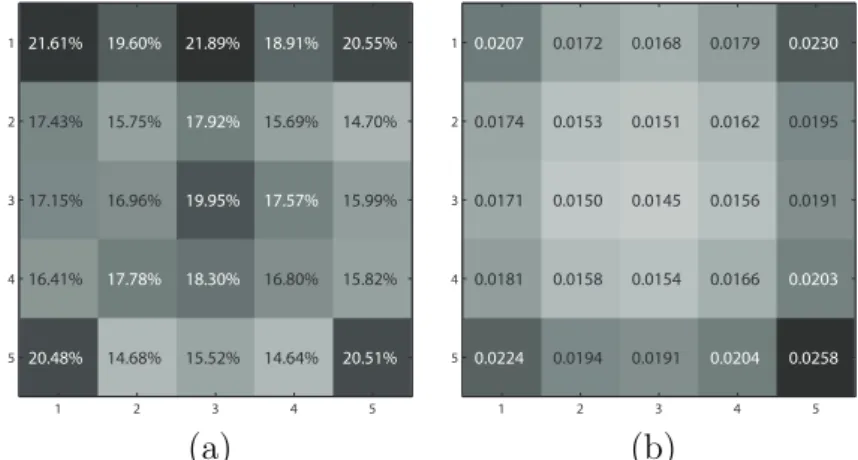
21.61% 19.60% 21.89% 18.91% 20.55% 17.43% 15.75% 17.92% 15.69% 14.70% 17.15% 16.96% 19.95% 17.57% 15.99% 16.41% 17.78% 18.30% 16.80% 15.82% 20.48% 14.68% 15.52% 14.64% 20.51% 1 2 3 4 5 1 2 3 4 5 0.0207 0.0172 0.0168 0.0179 0.0230 0.0174 0.0153 0.0151 0.0162 0.0195 0.0171 0.0150 0.0145 0.0156 0.0191 0.0181 0.0158 0.0154 0.0166 0.0203 0.0224 0.0194 0.0191 0.0204 0.0258 1 2 3 4 5 1 2 3 4 5 (a) (b)

Figure 2.7: (a). Percentages of pixel-wise RMSE reduced by our coupled training method compared with joint dictionary training method. (b) Pixel-wise RMSE of the recovered HR image patches (normalized and zero-mean) using our coupled dictionary training method.

To validate the effectiveness of our coupled dictionary training, we first compare the recovery accuracy of both dictionary training methods on a validation set, which includes 100,000 normalized image patch pairs sampled independently from the training set. Note that here we focus on evaluating the recovery accuracy for the zero-mean and normalized HR patch signal-s insignal-stead of the actual HR image pixelsignal-s, thusignal-s isignal-solating the affect of any

Learning sparse representation for image signals

ABSTRACT

ACKNOWLEDGMENTS

TABLE OF CONTENTS

CHAPTER 1

INTRODUCTION

CHAPTER 2

COUPLED SPARSE CODING FOR SINGLE

IMAGE SUPER-RESOLUTION

2.1

Introduction

2.2

Related Work

2.2.1

Sparse Coding

2.2.2

Joint Sparse Coding

2.3

Coupled Dictionary Learning for Sparse Recovery

2.3.1

Problem Statement

2.3.2

Formulation

2.3.3

Optimization for Dictionary

D

2.3.4

Sparse Derivative

2.3.5

Algorithm Summarization

2.4

Image Super-resolution via Sparse Recovery

2.4.1

Feature Extraction for SR

2.4.2

Patch-wise Sparse Recovery

2.4.3

Eﬃciency Improvements

2.5

From Sparse Coding to Deep Network

2.5.1

LISTA Network for Sparse Coding

ߠ

ܵ

+

ܵ

+

ߠ

ߠ

ܹ

ݕ

ߙ

ݖ

ݖ

2.5.2

Recurrent Network for Image SR

2.5.3

Network Cascade for Scalable SR

2.6

Experimental Results

2.6.1

Analysis of Coupled Dictionary Training