The energy costs of commuting: a
spatial microsimulation approach
by
Robin Lovelace, MSc BSc
A thesis submitted as partial fulfilment of the requirements for the degree of Doctor of Philosophy
in the
Faculty of Social Sciences Department of Geography
que se encuentra a 50 o 60 km de distancia. Este hecho, que para tal ciudadano formaba parte de la rutina de su vida cotidiana, constituye, sin duda, uno de los m´as grandes enigmas de la antropolog´ıa y la historia”
Jos´e Ardillo, El Salario del Gigante
“Towards the end of the 20th century, and thanks to the private automobile, a simple worker could live in one place but carry out their work, daily, 50 to 60 km away. This fact, which for the citizen formed part of their everyday routine, constitutes, without doubt, one of the greatest enigmas of Anthropology and History”
Commuting is a daily ritual for a large proportion of the world’s population. It is important materially, consuming large amounts of time, money and natural resources. As with many routine activities travel to work is often taken for granted but its energy consumption is of particular interest due to its heavy reliance on fossil fuels and the inflexibility of the demand for commuting. This understudied area of knowledge, the energy costs of travel to work, forms the basis of the thesis.
There is much research into commuting and transport energy use as separate fields, but they have rarely been combined in the same analysis, let alone at high levels of geographical resolution. The well-established field of spatial microsimulation offers tools for investigating commuting patterns in detail at local and individual levels, with major potential benefits for transport planning. For the first time this method is deployed to study commuter energy use between and within small administrative zones.
The maps of commuter energy use presented in this thesis illustrate this variability at national, regional and local levels. Supporting previous research, the results suggest that a range of geographical factors influence energy use for travel. This has important policy implications: when high transport energy use in commuting is due to lack of jobs in the vicinity, for example, modal shift (e.g. from cars to bicycles) on its own has a limited potential to reduce energy costs. Such insights are quantified using existing aggregate data. The main methodological contribution of this work, however, is to add individual-level factors to the analysis — creating the potential for policy makers to also assess the distributional impacts of their interventions and target specific types of commuters having high transport energy costs, rather than treat areas as homogeneous blocks. This potential is demonstrated with a case study of South Yorkshire, where commuting energy use is cross-tabulated by socio-economic variables and disaggregated over geographical space. The areas where commuting energy use is less evenly distributed across the population, for example in urban centres, are likely to benefit most from policies that target the specific groups. Areas where commuter energy use is more even, such as Stocksbridge (in Northwest Sheffield), will benefit from more universal policies.
The thesis contributes to human knowledge new information about the energy costs of commuting, its variability at various levels and insight into the implications. New methods of generating and analysing individual-level data for the analysis of commuter energy use have also been developed. These are reproducible (see the GitHub repository “thesis-reproducible” for example code and data) and will be of interest to researchers and policy makers investigating the energy security, resource efficiency and potential welfare impacts of interventions in personal travel systems.
It should be acknowledged at the outset that some parts of the thesis have been pub-lished:
• Parts of section 4.5 have been published in Computers, Environment and Urban Systems (Lovelace and Ballas, 2013).
• The tutorial “Spatial microsimulation in R”, a supplement to Lovelace and Ballas (2013), is based on Section 4.5.3.
• The results presented in chapter 7 have been published in theJournal of Transport Geography (Lovelace et al., 2013).
• Results presented in chapter 8 have been published in Geoforum (Lovelace and Philips, 2014).
Thanks to my supervisors Dimitris Ballas, Matt Watson and Stephen Beck for unceasing encouragement and guidance throughout. Dimitris has been instrumental in developing the methodological direction of the PhD project. I will be forever grateful for the guidance provided in the research and beyond.
Many thanks to Carlota for keeping my spirits up throughout. To Engineers Without Borders for allowing me to get my hands dirty, a feature too often missing from modern research. To my house-mates for providing a fun and homely habitat in Sheffield. To my parents, who instigated trips into the Peak District — the ultimate antidote to square-eyes. To my dear friends in Sheffield, especially James Folkes for providing pedal-powered entertainments and Joseph Moore for ‘moore’ distractions.
Thanks to the E-Futures Doctoral Training Centre. E-Futures was vital to this PhD, not only for providing funding that allowed its students financial security to dedicate themselves to study. E-Futures also provided a forum for debate. The encouragement from peers and across disciplines was inspirational. Neil Lowrie deserves special mention here, as he helped channel my energy away from confrontations with coal-fired power station operators and towards research. Thanks.
Thanks to the Department of Geography, for providing an academic home and a quiet desk. Members of the Social and Spatial Inequalities group (SASI), especially, provided feedback on my work, and encouraged the investigation of how commuting affects people, not just energy. I thank Luke Temple and Mark Green in particular in this regard. Thanks to the open source software movement in general and to the developers of R and LATEX (in which the document was written) in particular. Hadley Wickham stands
make the methods and results more accessible and reproducible for others.1
The thesis has benefited from the feedback of people who read early drafts of various sections and chapters: Milan Delor, Ian Philips, Jake Gower, Chris Hunter, Charlotte Bjork and my father David Lovelace. Dan Olner’s input was especially beneficial in the final stages. Thanks to all for providing additional feedback and support outside of the usual academic channels.
My penultimate thank you is for writers who awoke my interest in this topic: Ivan Illich, John Michael Greer, Howard T. Odum, George Monbiot and Vaclav Smil.
The final thank you is to the examiners of the thesis, Charles Pattie and Michael Batty.
1
Sample code and data used can be found ongithub.com/Robinlovelace/. In particular, reproducible versions of the results can be found in thethesis-reproduciblerepository.
Abstract iv
Acknowledgements v
Table of Contents vii
List of Figures xi
List of Tables xv
Abbreviations xvii
Symbols xix
1 Introduction 1
1.1 The ‘Big Picture’ . . . 1
1.1.1 Climate change . . . 2
1.1.2 Peak oil and resource depletion . . . 8
1.1.3 Inequality and well-being . . . 10
1.2 Commuter energy use: everyday realities . . . 12
1.3 The importance of commuting . . . 15
1.3.1 Trips . . . 15
1.3.2 Distance . . . 15
1.3.3 Time . . . 17
1.4 Thesis overview . . . 18
1.5 Aims and objectives . . . 19
1.5.1 Aims . . . 20
1.5.2 Objectives . . . 20
1.5.3 Methods . . . 21
2 Personal transport, energy and commuting 23 2.1 The sustainable mobility paradigm . . . 24
2.1.1 Active travel . . . 27
2.2 Commuting research: individual to national levels . . . 29
2.2.1 Personal factors: psychology, family and community . . . 30
2.2.2 Behavioural economics and its impacts on commuting . . . 31
2.2.3 The local and regional economy . . . 33 vii
2.2.4 National and global considerations . . . 35
2.3 Energy use and CO2 in transport studies . . . 36
2.3.1 The energy costs of urban form: urban sprawl and compact cities . 38 2.3.2 The energy costs of different transport modes . . . 38
2.3.3 The climate impacts of transport . . . 40
2.4 The energy impacts of commuting . . . 42
2.5 Commuting and energy use research: tools of the trade . . . 43
2.5.1 ‘Scientific’ approaches to energy and transport . . . 44
2.5.2 Visualisation methods . . . 46
2.5.3 Harnessing the ‘data deluge’ . . . 47
2.6 Concepts in energy and commuting . . . 47
2.7 Summary of the literature . . . 49
3 Spatial microsimulation and its application to transport problems 51 3.1 Definitions: what is spatial microsimulation? . . . 52
3.2 The history of spatial microsimulation . . . 56
3.2.1 Pre-computer origins . . . 56
3.2.2 The digital revolution . . . 59
3.2.3 Statistical methods for estimation . . . 60
3.2.4 Modern spatial microsimulation . . . 63
3.3 Spatial microsimulation: state of the art . . . 64
3.3.1 Types of spatial microsimulation models . . . 64
3.3.2 Reweighting algorithms . . . 65
3.3.3 Transport applications . . . 67
3.4 Microsimulation in urban modelling . . . 69
3.4.1 Dedicated transport models . . . 70
3.4.2 Land-use transport models . . . 72
3.5 Summary: research directions and applications . . . 73
4 Data and methods 77 4.1 Introduction . . . 77
4.2 Energy use data . . . 81
4.3 Social survey data . . . 83
4.3.1 Geographically aggregated data . . . 84
4.3.2 The Understanding Society dataset . . . 88
4.3.3 The National Travel Survey . . . 89
4.3.4 Other commuting datasets . . . 93
4.4 Geographical data: infrastructure and environment . . . 95
4.4.1 Infrastructure . . . 95
4.4.2 Topographic data . . . 100
4.4.3 Remoteness . . . 101
4.5 Building a spatial microsimulation model in R . . . 103
4.5.1 Why R? . . . 105
4.5.2 IPF theory: a worked example . . . 107
4.5.3 Implementing IPF in R . . . 111
4.6 Model checking and validation . . . 118
4.6.2 Model validation . . . 120
4.6.3 Additional validation methods . . . 125
4.7 Integerisation . . . 127
4.7.1 Method . . . 128
4.7.2 Results . . . 138
4.7.3 Discussion and conclusions . . . 142
5 Energy use in personal travel systems 145 5.1 Fundamentals of energy use in transport . . . 147
5.1.1 The factors driving energy use in transport . . . 149
5.1.2 System boundaries . . . 149
5.1.3 Early quantifications of energy use in transport . . . 152
5.2 Direct energy use: published estimates . . . 153
5.3 Calculating system level energy use . . . 157
5.3.1 The embedded energy of fuel . . . 159
5.3.2 Vehicle manufacture . . . 164
5.3.3 Guideway manufacture . . . 168
5.4 Additional factors affecting energy use . . . 170
5.4.1 Frequency of trip . . . 171
5.4.2 Occupancy . . . 175
5.4.3 Efficiency impacts of trip distance . . . 177
5.4.4 Circuity . . . 179
5.4.5 Efficiency impacts of congestion . . . 182
5.4.6 Behaviour . . . 184
5.4.7 Environmental conditions . . . 185
5.5 Variability over time . . . 187
5.5.1 The improving fleet efficiency of cars . . . 187
5.5.2 Modal shift . . . 190
5.5.3 Future efficiency improvements . . . 194
5.6 Variability over space: local fleet efficiencies . . . 198
5.7 Final energy use estimates . . . 204
6 The energy costs of commuting 207 6.1 Commuter energy use at the national level . . . 208
6.2 Regional and sub-regional patterns . . . 212
6.3 Total commuting energy use and comparisons with other sectors . . . 218
6.4 Local and individual level variability . . . 223
6.4.1 A case study from South Yorkshire . . . 224
6.5 A comparison of commuter energy use in England and the Netherlands . . 227
6.5.1 Data, method and results . . . 229
6.5.2 Explaining Dutch commuter energy use . . . 231
6.5.3 Data inconsistencies and caveats . . . 233
6.6 Discussion . . . 235
7 Social and spatial inequalities in commuter energy use 237 7.1 The importance of distributional impacts in transport studies . . . 237
7.3 Assigning work location . . . 244
7.4 Model validation . . . 247
7.5 Results . . . 250
7.6 Discussion . . . 255
8 Scenarios of change 259 8.1 Modal shift: ‘going Dutch’ . . . 261
8.1.1 An aggregate level model of modal shift . . . 262
8.1.2 A spatial microsimulation implementation . . . 265
8.1.3 Taking the scenario further . . . 267
8.2 Reducing commute frequency: ‘going Finnish’ . . . 268
8.3 Reduction in commute distance: ‘eco-localisation’ . . . 271
8.4 Oil vulnerability . . . 273
8.4.1 Metrics of vulnerability: resources, jobs, money . . . 274
8.4.2 Results: trips, distance and energy use . . . 277
8.4.3 Local and individual level results . . . 280
8.5 Discussion: policy relevance and limitations . . . 284
8.5.1 Policy relevance of findings . . . 285
8.5.2 Limitations of the approach . . . 287
9 Conclusions 291 9.1 Methodological contribution . . . 292
9.2 Policy relevance and limitations . . . 294
9.3 Summary of findings . . . 295
9.4 Further work . . . 297
9.5 Thesis evaluation and summary . . . 299
Bibliography 303
1.1 UK transport emissions by source in 2009 (DECC, 2011c). . . 3
1.2 The greenhouse gas emissions per unit energy of various fuels . . . 6
1.3 Biofuels’ contribution to global transportation energy use . . . 9
1.4 Average prices of Brent Crude oil spot prices, 1992 – 2012 . . . 10
1.5 UK Gini index for market and disposable income in context (OECD, 2011). 11 1.6 Commuting options to Tyrrell’s crisp factory . . . 13
1.7 Average number of trips per person per year across Great Britain. . . 16
1.8 Average trip length by purpose in Great Britain. . . 16
1.9 Total distance travelled by mode in Great Britain. . . 17
1.10 Time spent commuting in Great Britain . . . 18
2.1 The sustainable transport hierarchy (Kay et al., 2011). . . 26
2.2 Proportion of trips by active travel by distance and mode . . . 29
2.3 Schematic for organising research commuting research by scale. . . 30
2.4 Energy performance of different modes, from (Radtke, 2008). . . 39
3.1 Schematic a transport simulation model . . . 53
3.2 MATSim schema (permission: Michael Balmer) . . . 71
4.1 Idealised data schema for studying energy use in commuting . . . 78
4.2 Questions 33 and 34 of the 2001 UK Census . . . 83
4.3 National, regional and city-wide scales of analysis . . . 85
4.4 Cross-tabulated dataset containing mode/age/sex variables . . . 87
4.5 Bar-plot of frequency of working from home . . . 92
4.6 Schematic of transport networks and vehicles . . . 96
4.7 Visualisation of the OSM data source of the transport network. . . 97
4.8 The Meridian 2 transport network dataset. . . 98
4.9 The Ordnance Survey’s Integrated Travel Network dataset. . . 99
4.10 Distribution of employment in Sheffield . . . 103
4.11 Illustration of how distance to employment centre was calculated. . . 104
4.12 Scatter plot of the fit between census and survey data . . . 115
4.13 Scatter plot showing the fit after constraining by age. . . 117
4.14 Improvement of model fit with iterations . . . 117
4.15 Diagnostic plot to check the sanity of age and sex inputs. . . 119
4.16 Diagnostic plots to identify model error . . . 120
4.17 Scatter plot of simulated vs official estimated income . . . 122
4.18 Scatter plot of error introduced in Nomis data . . . 124
4.19 Errors associated with Casweb census variables . . . 124
4.20 Scatter plot of the proportion of male drivers . . . 125
4.21 Overplotted scatter graph showing the distribution of IPF weights . . . . 131
4.22 Histograms of original microdata and integerised weights . . . 133
4.23 Overplotted scatter graphs of index against weight . . . 135
4.24 Scatter graph of the index values of individuals . . . 135
4.25 Visualisation of IPF method . . . 137
4.26 Scatter graph illustrating the fit between census and simulated aggregates 137 4.27 Scatterplots of actual (census) and simulated population totals . . . 139
5.1 Schematic diagram of the factors causing energy use in transport. . . 150
5.2 Relative importance of fixed and variable costs of car ownership . . . 151
5.3 Schematic of physical system boundaries in personal transport systems. . 152
5.4 Screen shot of the spreadsheet used to calculate system level energy costs. 159 5.5 UK transport energy consumption by mode and energy source . . . 163
5.6 Iron ore mine and 3D CAD images of two modern car engines . . . 165
5.7 Frequency of trips to work each week, by distance . . . 172
5.8 Proportion of trips by distance for different trip frequencies . . . 173
5.9 Relationship between trip frequency and distance . . . 174
5.10 Average car occupancies over time in three regions . . . 177
5.11 The impact of car speed on efficiency, from (Anas and Hiramatsu, 2012). . 178
5.12 Line graph of energy intensity vs trip distance . . . 179
5.13 Schematic of Euclidean and network distances . . . 179
5.14 The decay of circuity with distance travelled . . . 180
5.15 EU test cycle . . . 182
5.16 Urban and extra-urban energy use of selected models . . . 183
5.17 The commuting ‘rush hours’ . . . 184
5.18 Fleet efficiency of UK vehicles over time . . . 189
5.19 Comparison of UK car fleet efficiency estimates over time (DfT, 2013). . . 190
5.20 Fleet efficiencies of new cars in the UK and USA, 1977-2012 . . . 191
5.21 Mode of transport to work, 1890-1990 . . . 192
5.22 Estimates of energy use per commuter trip, 1890-1990 . . . 193
5.23 Modal split of travel to work over two decades . . . 193
5.24 The growing dominance of the car, 1981 to 2001 . . . 194
5.25 Fuel energy use of future car technologies . . . 195
5.26 Barpolt of 2001 car registrations by emission band . . . 201
5.27 Scatterplots of estimated fleet efficiencies at MSOA level . . . 202
5.28 Car fleet efficiencies in Yorkshire and the Humber in 2001 . . . 203
5.29 Final energy use estimates, from a range of sources. . . 205
5.30 Fuel energy use of UK transport modes, 1991 . . . 206
6.1 Distance bands and average distance travelled for motorised modes . . . . 211
6.2 Distance bands and average distance travelled for active modes . . . 212
6.3 Mode and distance categories of commute in England . . . 213
6.4 Comparison of commute energy costs between England and Wales. . . 213
6.5 Average energy use per trip (Etrp, in MJ) in English regions . . . 214
6.6 Raw count data of commuters by mode and distance. . . 214
6.8 Average energy use per commuter trip at the district level . . . 217
6.9 Average energy use per trip (Etrp, in MJ) in English wards . . . 218
6.10 Proportion of energy use caused by train trips . . . 219
6.11 Proportion of total energy use in the UK consumed by commuting . . . . 221
6.12 Proportion of transport energy use in the UK consumed by commuting. . 222
6.13 Commuter energy use in South Yorkshire. . . 226
6.14 Proportion of energy used for commuting by the top 20% . . . 226
6.15 Relative energy use by top social classes . . . 228
6.16 Comparison of commuter energy use in England and the Netherlands . . . 230
6.17 Modal split of commuter trips in England and the Netherlands . . . 231
6.18 Distance of commuting by mode, England and the Netherlands . . . 232
6.19 Population density against commuter energy use . . . 233
6.20 Average commuter trip distance over time in Great Britain . . . 234
6.21 Modal split of commuter trips, Great Britain 1995 - 2009 . . . 234
7.1 Trip distance and mode by household income . . . 238
7.2 Heatmap of mode of travel by income group . . . 239
7.3 Fit between simulated and census data . . . 243
7.4 Employment density at the local level in Sheffield . . . 244
7.5 Flow diagram of commuter destinations from Stocksbridge . . . 245
7.6 Simulated route choice for 20 randomly selected individuals . . . 246
7.7 Circuity as a function of distance in Sheffield . . . 247
7.8 Comparison of census and simulated results at the aggregate level . . . . 248
7.9 Mean equivalised household income from official and simulated data . . . 249
7.10 Proportion of trips, distance, and energy by mode . . . 252
7.11 Average distance travelled to work in Yorkshire and the Humber . . . 253
7.12 Average distance to employment centre in South Yorkshire . . . 253
7.13 Scatter plot of distance vs energy costs in Yorkshire and the Humber . . . 254
7.14 a) Income and household traits; b) Lorenz curves of commute distances . 256 7.15 Low-income car-free families and bus-stops in South Yorkshire . . . 257
8.1 Estimated energy savings from car-bicycle modal shift . . . 264
8.2 The relationship between age and bicycle use . . . 266
8.3 Energy savings from car-bike modal shift in South Yorkshire . . . 267
8.4 Differences between individual and aggregate level implementations . . . . 268
8.5 Energy savings from telecommuting scenario in South Yorkshire. . . 270
8.6 Vulnerability of commuter patterns in Yorkshire and the Humber . . . 278
8.7 Scatterplot matrix of vulnerability metrics . . . 279
8.8 Chloropleth map of deprivation in Yorkshire and the Humber . . . 280
8.9 Distance to employment centre from zone centroids . . . 281
1.1 Top 5 UK sectors in terms of greenhouse gas emissions, 1990-2010 . . . . 4
3.1 Typology of spatial microsimulation methods . . . 65
3.2 Five entities central to urban modelling, after Wilson (2000) . . . 69
4.1 Sample of regional transport energy consumption statistics . . . 82
4.2 Aggregate data on energy costs of commuting by scale . . . 85
4.3 Selected individual level variables related to commuting . . . 89
4.4 Comparison of data sources for travel networks . . . 97
4.5 A hypothetical input microdata set . . . 108
4.6 Hypothetical small area constraints data (s). . . 108
4.7 Small area constraints expressed as marginal totals . . . 108
4.8 The aggregated results of the weighted microdata set . . . 109
4.9 Reweighting the hypothetical microdataset in order to fit Table 4.6. . . . 109
4.10 Aggregated results after constraining for age . . . 110
4.11 Summary data for the spatial microsimulation model . . . 136
4.12 Accuracy results for integerisation techniques.* . . . 141
4.13 Differences between census and simulated populations. . . 142
5.1 The direct and indirect energy costs of personal travel (Fels, 1975) . . . . 153
5.2 Direct energy use of selected modes . . . 154
5.3 Direct greenhouse gas emissions by mode . . . 154
5.4 Conversion table from emissions to energy use by size of car . . . 155
5.5 Emissions data and calculated energy use of motorised modes . . . 157
5.6 Estimates of the energy costs of car manufacture (EMv) . . . 167
5.7 Average frequency of trips for Euclidean distance bins . . . 173
5.8 Average occupancy of car journeys by reason for trip . . . 176
5.9 Vehicle emissions bands of registered vehicles since 2001 . . . 199
5.10 Average energy usage of cars by tax band . . . 200
5.11 Correlation matrix of estimated fleet efficiencies, 2002-2010 . . . 201
5.12 The first 5 rows of the raw DfT emissions band data . . . 203
5.13 Final estimates of the direct and indirect energy use of 8 modes . . . 204
6.1 Average distance travelled by mode and distance band . . . 210
6.2 Correlation matrix of energy use for commuting and emissions . . . 222
6.3 Sample of the spatial microsimulation model output . . . 224
6.4 Sample of individual level spatial microsimulation output . . . 225
6.5 Commuter energy use in South Yorkshire areas by class . . . 227 6.6 Comparison of basic national attributes in England and the Netherlands . 229
6.7 Sample of the raw Dutch commuting data . . . 230
7.1 Aggregate level inputs into the spatial microsimulation model . . . 243
7.2 The 2nd most common mode of commuting compared with other factors . 246 7.3 Summary statistics of the commuting behaviour of in South Yorkshire . . 250
7.4 Contingency table of variables related to commuting . . . 255
7.5 Commuting characteristics cross-tabulated by income bands . . . 255
8.1 Proportion of trips (T), distance (D) and energy (E) by mode . . . 277
8.2 Summary statistics of vulnerability metrics . . . 283
8.3 Individual level characteristics of ‘oil vulnerable’ commuters . . . 284
8.4 Differences between commuters affected by the ‘Dutch’ and ‘Finnish’ sce-narios . . . 287
Acronym What it Stands For kJ kilojoules (103 J) MJ megajoules (106 J) GJ gigajoules (109 J) TJ terajoules (1012 J) PJ petajoules (1015 J) EJ exajoules (1018 J) kWh kilowatt hour (3.6 MJ) CO2 Carbon dioxide
EROI Energy return on (energy) investment IPF Iterative proportional fitting
pkm passenger-kilometres vkm vehicle-kilometres
TRS Truncate replicate sample (integerisation method)
DECC Department of Energy and Climate Change
Defra Department for Environment Food & Rural Affairs NTS National Travel Survey
ONS Office for National Statistics OSM Open Street Map
USd Understanding Society dataset
symbol name unit
dE Euclidean distance km
dR route distance km
Etrp direct primary energy use per trip J
ET total energy use of all commuter trips in a given area GJ
ET yr total primary energy per year GJ/yr
Esys total primary energy use (direct and indirect) MJ/km
Ef Direct fuel (including electricity and food) energy use per kilometre MJ/vkm
Ef p Energy costs of fuel production MJ/vkm
Ev Energy costs of vehicle production per unit distance MJ/vkm
Eg Energy costs of guideway construction per unit distance MJ/vkm
EM v embodied energy of vehicle production GJ/vehicle
EM g embodied energy of guideway production GJ/km
EI energy intensity of transport per passenger kilometre MJ/pkm
F E fuel economy of vehicle L/100 vkm
Lf load factor of vehicle or mode
Lg lifespan of guideway vehicle passes
Lv lifespan of vehicle vkm
m mode of transport (e.g. car, train)
Oc occupancy, the number of people in each vehicle people/vehicle
P power W (Js−1)
Q circuity: route distance divided by Euclidean distance
η energy conversion efficiency (Energy outEnergy in)
T oe tonnes of oil equivalent
Introduction
The research presented in this thesis focuses on commuting and its energy costs. UK datasets from the beginning of the 21st century form the empirical foundation of the work. Travel to work statistics are described, analysed and in later chapters modelled to assess the variability of energy use for this commuting. The underlying motivations are broader and play an important role throughout the thesis, from the choice of method-ology (chapter 4) to the specification for scenarios of change (chapter 8). It is therefore important to lay out these wider issues at the outset, before highlighting the impact of commuting at the individual and national scale (in sections 1.2 and 1.3). These ‘big picture’ motivations also inform the research aims and objectives (section 1.5).
1.1
The ‘Big Picture’
Our increasingly interconnected global civilisation is facing challenges that are unique in the history of humankind. Environmental and social-economic changes are occurring to a greater extent and faster than ever before (Rifkin, 2011; Ehrlich and Ehrlich, 2013). Perhaps more importantly, this generation is in the privileged position of being able to monitor, predict and respond to these changes as they occur (Evans, 1998; Smil, 2008; IPCC, 2007). This work is firmly situated in the context of these changes and aims to contribute to humanity’s understanding of them. Following the academic tendency for specialisation whilst avoiding the pitfalls of dogmatic allegiance to any particular discipline or worldview (Kates and Burton, 1986), this thesis focuses on one ‘bite-sized’ yet important part of these wider issues.
Energy intensive transport contributes to pressing environmental, social and economic problems of the 21st century. Climate change, resource depletion, and growing levels of
economic inequality are global problems aggravated by energy use. Travel is a major energy consumer. Yet transport systems powered by fossil fuels have become integral to modern life: by the 1970s ‘automobility’ was central to social change (Illich, 1974) and since then motorised transport has become even more central to modern life (Rodrigue et al., 2009). This means that policy-makers, businesses, and individuals will have to make difficult decisions in the coming decades. According to some the situation is urgent: “Rapid decisions now need to be made so that the impacts of transport on the environment can be minimised and fossil fuel resources conserved” (Chapman, 2007, p. 354). Rapid decisions are not alwaysgood decisions, however: rational choices depend on good information about the world.
Because of the scale and complexity of the previously mentioned global problems, it is tempting to focus solely on the detail of energy use in commuting as one aspect of personal travel about which good datasets are available. It is however important to understand the wider context of transport energy use in order to decide the most useful applications of and directions for future research in this area. An introduction to the broader context that motivates this research is therefore provided, focussing on the three ‘big issues’ of climate change, peak oil, and economic inequality which are also long-term political priorities in the UK (UKERC, 2010).
1.1.1 Climate change
The Earth’s climate has always changed: it is a complex system with non-linear re-sponses to internal and external drivers and a number of feedback loops (IPCC, 2007). The changes during the 20th and 21st centuries are, however, different from those ob-served in the paleoclimate record: “It is important to realize that the current change in atmospheric CO2 is proceeding at a rate more than 200 times faster than any natural
change in Earth’s past history, except the Cretaceous-Tertiary boundary event gener-ally attributed to impact of an asteroid with the Earth” (Hay, 2011). The other major difference is that today climate change is caused by the combustion of fossil fuels by humans. Commuting, composed of millions of motorised trips to work and back each day, is a small yet important contributor. The desire to reduce these emissions, for the maintenance of a “safe operating space for humanity” (Rockstrom et al., 2009) provides an important motivation for this research. An underlying aim is to contribute ideas and information to the ongoing debate about how to mitigate anthropogenic climate change (Matschoss and Kadner, 2011).
This aim appears to be shared by others: academic interest in transport emissions has proliferated in recent years (Akerman et al., 2006; Chapman, 2007; Schwanen et al.,
2011), although less so in the specific area of commuting (chapter 2). Because energy use is directly related to greenhouse gas emissions (Mackay, 2009), this research is also about climate change.
UK greenhouse gas emissions
At the UK level, the emissions associated with commuter energy are subsumed within ‘transport emissions’. These include emissions from shipping, aviation and military transport, as well as the road and rail sectors (DECC, 2011c). Road transport dominates, accounting for more than 90% of the UK’s transport emissions (figure 1.1).
Figure 1.1: UK transport emissions by source in 2009 (DECC, 2011c).
An interesting feature of the UK’s emissions reporting strategy is that ‘transport’ is generally presented as a monolithic category (e.g. DECC, 2010), despite the wide variety of transport modes and purposes presented in figure 1.1. This makes it difficult to identify the specific drivers of growth in UK transport emissions since 1970 (Gasparatos et al., 2009) and stagnation since 1990 . What is clear in both cases is that energy use and hence emissions from transport have increased (since 1970) or stagnated (since 1990) while those of other sectors have declined. Between 1990 and 2010, transport was the only sector other than housing in which emissions increased; transport now accounts for just over 20% of UK emissions (table 1.1, below). This research project quantifies the contribution of commuting to this total in terms of energy use, and provides evidence about which strategies may be effective for reducing the emissions due to transport to work.
The UK’s climate change commitments are unambiguous, agreed upon by all major parties, and legally binding: emissions in 2050 must be below 20% of their 1990 level (Committee on Climate Change et al., 2008). This means that the total permitted
emissions in 2050 across all sectors are roughly equal to the emissions from just the transport sector today. This fact underlines the scale of the proposed changes: transport to work represents a small but important component of this challenge that affects millions of working people every day.
Table 1.1: Top 5 UK sectors in terms of greenhouse gas emissions, 1990-2010 (MtCO2e). Data from DECC (2011a)
1990 2000 2010 % change % emissions (2010) Energy Supply 273.4 220.1 204.3 -25.3 34.8 Transport 121.5 126.7 121.9 0.3 20.7 Residential 80.8 90.1 89.9 11.3 15.3 Business 113.2 111.3 89 -21.4 15.1 Agriculture 63.1 58 50.7 -19.7 8.6 Other 117.4 65.8 32 -72.7 5.4 Total 769.4 672 587.8 -23.6 100.0
Emissions from transport to work
Of the 20% of UK emissions that arise from transport, only a small fraction are due to transport to work. How small? No official breakdowns of emissions are provided by reason for trips, but estimates can be made by analysing the make-up of the transport sector. As shown in figure 1.1, 5% of transport emissions can be accounted for by military vehicles, aviation and shipping: none of these are usually involved in transport to work. Also, 31% of road transport emissions arise from goods vehicles (HGVs and LGVs); the remaining 69% arise from road vehicles for personal transport – buses, motorcycles and cars (DECC, 2011b). From these figures, it is possible to estimate that 80 MtCO2e
result from personal travel in the UK. 19.5% of passenger kilometres travelled by all personal transport modes in the UK are due to travel to work (DfT, 2011b). Transport to work can be estimated to cause∼16 MtCO2e of emissions or around 3% of the UK’s
total. (In section 6.3 a more refined estimate of commuter energy use is presented, based on geographically disaggregated data: commuting was found to account for 4.1% of total energy use and 14.4% of transport energy use.)
It is important to undertake such ‘back of the envelope’ calculations at the outset of research into emissions reduction strategies or sustainable energy to ensure that time is not wasted on negligible issues such as phone chargers (Mackay, 2009). David MacKay, Chief Scientific Advisor at the Department of Energy and Climate Change (DECC), puts this argument in lay terms by proposing a rule for energy-saving interventions: “A gizmo may be discussed only if it could lead to energy savings of at least 1% ... because the public conversation about energy surely deserves to be focussed on bigger fish” (MacKay, 2009). Applying this reasoning more broadly to areas of energy use,
transport to work clearly deserves attention according to this rule, although emissions cuts in commuting will have to be matched in all other sectors for targets to be met. However, there are reasons to believe that making cuts in the transport sector generally, and in transport to work in particular, will be especially difficult, and therefore worthy of dedicated investigation. These include:
• The transport sector is overwhelmingly dependent on petrol and diesel: motorised transport (which accounts for most trips and the vast majority of the distance travelled, as shown in chapter 5) is 95% dependent on refined oil products (Wood-cock et al., 2007). This is problematic because there are no commercially viable, low emissions alternatives to crude oil for liquid fuels. Biofuels are the only ‘re-newable’ option on the table, but their potential contribution is low (Grady et al., 2006; Michel, 2012), they can conflict with food production (Pimentel et al., 2009), and currently used crops may increase greenhouse gas emissions due to land use change (Fargione et al., 2008).
• Linked with the previous point, low carbon technology is far less promising in the transport sector than in other large emitting sectors. For electricity generation and residential heating the technologies for renewable alternatives are becoming more commercially viable (Chu and Majumdar, 2012). By contrast, the penetration of electric, hydrogen, and biofuel-powered cars may be slow, largely due to their high cost (Proost and Van Dender, 2011; Vaughan, 2011).
• The current transport system is built around road (and to a lesser extent rail) infrastructure that took many decades and large capital investments to complete. The dependence of society on the car is deeply embedded, yet a low-energy (and hence low emissions) transport system may require a shift away from personal ownership of automobiles altogether (Mackay, 2009; Moriarty, 2010), something that will take decades to accomplish.
These difficulties make de-carbonising transport systems problematic compared with the other large energy users — electricity and heat production.1 Despite these issues, transport is rarely framed in terms of energy use and greenhouse gas emissions (chap-ter 2). In addition to its impacts on climate change via direct and indirect greenhouse gas emissions, commuting is also vulnerable to the effects of climate change, as discussed in section 8.5.2.
1These can convert more easily to renewable sources — e.g. via stationary wind turbines and solar hot water panels — than can transport systems. This is because transport systems are inherently mobile, therefore requiring a high energy density power source. Fossil fuels are unrivalled in terms of their energy density — almost 100 times greater than the best non-agrofuel commercial alternative: lithium ion batteries. Hydrogen fuel cells have been proposed as a solution, but these are still far from commercial viability, and have been precluded by DECC’s Chief Scientific Advisor on the grounds that they are highly inefficient (Mackay, 2009).
1.1.1.1 Climate change and energy
Most studies looking at the impact of one aspect of the economy on climate change do so through the emissions that it produces. These studies generally measure environmental impact in terms of kilograms of carbon or CO2 equivalent caused by different modes of
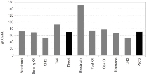
travel. This seems logical if one is concerned about climate change: it is the greenhouse gases that trap the heat (Houghton et al., 1990). However, others have suggested that the best way to tackle the problem is from an energy perspective: “climate change is an energy problem”, as a group of 18 prominent US academics put it (Hoffert et al., 2002, p. 981). What is meant by this is that energy use and greenhouse gas emissions are currently two sides of the same coin. More than 80% of commercial total primary energy supply (TPES) worldwide is provided by fossil fuels (Smil, 2008) and in the transport sector this is even higher. It is true that not all forms of energy have the same emissions. Yet, as illustrated in figure 1.2, CO2 emissions per unit energy are in fact
surprisingly similar across a wide range of transport fuels. In addition, even if it were possible to decarbonise electricity production in the near-term, the fact remains that uptake of low-energy sources will almost certainly be gradual (Smil, 2010b). Another issue is that technologies that have low emissions per unit of energy use during the usage phase of their lifecycle often have an energy intensive production phase. Because much modern food production depends upon fossil fuel energy, the energy approach can also help in the assessment of wide-boundary energy impacts. Some environmental impacts of transport such as noise, road-kill and the need to frequently resurface roads pummelled by powerful vehicles are not included in most emissions estimates. Energy use can to some degree encapsulate these additional impacts.
Figure 1.2: The greenhouse gas emissions per unit energy of various fuels. Data taken from Defra (2012) (additional sources forelectricity and biofuelemissions were used)
The reasons for advocating a focus on energy use, and not emissions directly, can be summarised as follows:
• Emissions can be variable depending on the energy/fuel source, whereas energy is constant across fuel sources.
• If energy use is reduced overall, carbon-intensive forms can be phased out. How-ever, if emissions from one sector fall, they may well rise in another as fossil energy resources are freed-up.2
• Energy is the ‘master resource’ from which all others (including more energy) can be obtained; emissions are the end result of energy use.
• It can be argued that energy use is at the root of the linked ‘big picture’ problems mentioned in this chapter, not just climate change. Therefore tackling the energy problem could have numerous co-benefits.
All this suggests that the climate debate should be much more closely linked to the energy debate. Specifically, the carbon content of proven fuel reserves should be compared with the carbon dioxide content that can safely be burned. Doing this analysis, based on recently released data on fossil fuel assets, has led to an alarming finding: “for all the talk about finite resources and peak oil, scarcity is resoundingly not the problem. From the climate’s perspective, there is far too much fossil fuel” (Berners-Lee and Clark, 2013, p. 29). Berners-Lee and Clark (2013) show that for there to be at least a 75% chance that the global temperature increase remains below two degrees humanity can burn only around a half of economically viable reserves. In terms of personal transport, this means phasing out petrol and diesel and avoiding carbon-intensive electricity sources: a fundamental shift.
Most greenhouse gas emissions stem from fossil fuel use, and once extracted, these fuels are invariably burned. This has led to the conclusion amongst some that the solution must be top-down: fossil fuel companies must be forced to leave most of their assets un-tapped. This can be achieved either through plummeting prices of fossil fuels or through regulation. The former case is currently highly unlikely due to the surge of fuel demand from emerging economies, combined with the sheer utility of fossil fuels.3 The latter also
2
For example, imagine if transport emissions rapidly dropped to zero due to electrification and rapid uptake of renewables. The additional load on the grid caused by this new user (Dyke et al., 2010) could lead to an increase in the emissions stemming from space heating because the total supply of renewable energy is fundamentally limited by the laws of physics (Mackay, 2009). Berners-Lee and Clark (2013) describe this problem with emission reduction plans overall as squeezing a balloon: savings in one area tend to bulge out in another.
3However, if governments, in coordination, prioritise minimising energy use while maximising uptake of renewable energy, the former possibility would become more feasible.
seems unlikely, following the failure of UN talks in Copenhagen to arrive at a consensus on legally binding and enforceable emission targets for the major emitter. This research is relevant in any case: if fuel prices remain high there is a strong economic incentive to reduce energy imports. If leaders worldwide agree to tackle climate change through top-down or bottom-up policies, there will clearly be a strong interest in how best to reduce reliance on fossil fuels in every sector that is vital for well-being. Regardless of the level of regulation (whether it occurs at the point of extraction or use of fuel), it implies high consumer prices for fuels, through policies such as taxes, a ‘carbon cap’ or even energy rationing.4 Another pragmatic benefit of the energy approach is that even if one questions the need to tackle climate change, the arguments to reduce dependence on finite fossil fuels for other reasons are very strong.
1.1.2 Peak oil and resource depletion
In addition to the impacts of climate change, depletion of our fossil energy resources is another non-negotiable reason for transition away from fossil fuels, to a “post-carbon” economy (Heinberg, 2005, 2009; Heinberg and Fridley, 2010; Kunstler, 2006). Oil is the most rapidly depleting resource yet motorised transport is almost entirely dependent on liquid fossil fuels derived from it (Gilbert and Perl, 2008). Multinational personal transport industries tend to downplay or deny the risks of peak oil, pointing to non-conventional oil resources and technological advance as reasons not to worry. Prototype biofuels, electric cars and hydrogen fuel cells are often cited as ways of overcoming high prices. This is ironic because each technology is highly dependent on oil for resource extraction, manufacture, distribution and waste disposal stages of their life-cycle: high oil prices could make the batteries for electric cars, to take one example, even more expensive, far out of the reach of the median global citizen. Each technology is still in the research phase of development, relies on scarce public subsidies to be commercially viable and cannot operate on the scale needed within modern transport infrastructures even if production lines producing them were scaled up before a major oil shock. Biofuels, to take the most heavily subsidised example, can only ever produce a small fraction of current transport energy demand even if all available resources were exploited to the maximum (figure 1.3).
For this reason peak oil is a major motivation for research into energy and transport. How will transport systems operate beyond 2050, when oil production will be a fraction of its current level? (Aftabuzzaman and Mazloumi, 2011). How will people get to work in the event of shortages? (Noland et al., 2006). These are just a couple of examples
4
Interestingly, high prices of fossil fuels is also the end result of many scenarios of resource depletion, which has historically been another major driver of research into energy and transport (Berry and Fels, 1973).
Figure 1.3: Biofuels’ current (2010) and potential contribution to global
transporta-tion energy use (Aleklett, 2012, p. 228). Image used with permission of author. Data originally presented in Johansson et al. (2010).
of the kinds of questions that are being asked in preparation for declining oil supply. A parallel question (explored in section 8.4) is: how will commuters be affected by oil price shocks, depending on where they live and their socio-demographic characteristics? The potential problems posed by peak oil for motorised transport systems are severe and include collapse of complex economic activity due to the highly inter-dependent nature of the global economy (Friedrichs, 2010; Korowicz, 2011). For this reason an introduction to peak oil, and how it relates to commuting, will help to place this research in the wider context. Gilbert and Perl (2008) provide a comprehensive reference on the subject, from a North American perspective.
Peak oil is the point at which global oil production enters terminal decline due to deple-tion of large oil fields (Greer, 2008). It is an inevitable event during the 21st century, as oil is a finite resource, approximately half of which has been used (Aleklett et al., 2010). However, there remains controversy about the exact timing of the peak (Smil, 2008). An in-depth review by the UK’s Energy Research Centre (UKERC, 2009) found that the weight of evidence suggests a peak in the near-term, before 2030. This is well before
the 20 years that the famous Hirsh Report (Hirsch, 2005) indicated would be needed to prepare for declining supplies of liquid fuel. The implications are stark: if peak oil does occur before 2030, as the evidence reviewed by UKERC (2009) suggests, urgent preparations must begin now.
As economists have long indicated (Solow, 1974), it is not only the amount of oil left in the ground that directly affects peoples’ lives. It is theprice of oil that affects transport systems, with knock-on impacts on human lives. Price is also affected by changes in demand and technologies for extraction and substitution (Perman, 2003). Over the past decade there has been increasing evidence that depletion plays a major role in determining global oil prices, however, with high and volatile prices likely in the future (Aleklett, 2012). The price of crude oil during the past 20 years has shown both volatility and (when a smoothed by a rolling average function) a near inexorable upward trend figure 1.4.
Figure 1.4: Average prices of Brent Crude oil spot prices per week, January 1992 until
October 2012 (dots) and a 2 year rolling average (blue line) Data from the U.S. Energy Administration (http://www.eia.gov/dnav/pet/pet_pri_spt_s1_d.htm) plotted
us-ing the R package ggplot2.
Despite these upward trends, UK government energy policies are still largely based on the assumption that oil prices will remain below $100 per barrel into the 2020s (UKERC, 2010). Thus methods that estimate the oil-reliance of households based on readily available commuter statistics could be highly relevant to politicians and planners making long-term decisions. The ability to quantitatively explore the impact of high oil prices
and other scenarios of change at the individual level is an output of this research that could have applications in transport policy evaluation and development. See chapter 7.
1.1.3 Inequality and well-being
Peak oil and climate change are important because we depend on the resources and pro-cesses of the natural environment to survive. Humans also depend on the relationships between each other, not simply for survival, but for quality of life. “It is only in the backward countries of the world”, wrote John Stuart Mill, “that increased production is an important object; in those most advanced, what is needed is a better distribution” (Mill 1857, in Perman 2003: p. 6).
With more than 150 years of hindsight, Mill’s statement seems all but Utopian: economic growth is still the number one priority of most governments worldwide, even in wealthy countries such as the UK where evidence suggests that further growth may do more harm than good, for people and the environment (Latouche, 2008). To such an extent does economic growth dominate modern decision making, regardless of consideration of how growth is distributed, that authors such as Charles Eisenstein and John Michael Greer refer to it as the founding story of our age (Eisenstein, 2011; Greer, 2009). In contrast to this dogmatic growth focus, evidence suggests that other things, including equality of economic and social opportunities, lead to quality of life (Jackson and Day, 2008; Jackson, 2009).
The growth-at-all-costs mentality, combined with our debt-based capitalist economy5 has caused inequalities to grow worldwide (OECD, 2011). The UK has one of the highest levels of inequality in Europe (figure 1.5).
This problem is important in the context of the energy costs of commuting because em-ployment opportunities are greatly affected by one’s ability to find and affordably travel to work. Variable transport opportunities amplify social and economic inequalities: 38% of jobseekers say transport problems prevent them from getting a job (Social Exclusion Unit, 2002). “No jobs nearby” and “lack of personal transport” were the first and second most frequently cited barriers to getting or keeping a job in a survey of young people in the UK (Bryson et al., 2000).
Paid employment, and the economic independence it brings, is a foundation for life satisfaction (Jahoda, 1982). Work is “a principal source of identity for most adults”
5
As explained by Eisenstein (2011), the very existence of positive interest rates ensures that those who have money tend to have more. According to this view, growing levels of economic inequality is built into the monetary system, and can only revert back to low levels with crises such as wars or depressions, planned debt annulments or (preferably for Eisenstein) negative interest rates.
Figure 1.5: UK Gini index for market and disposable income in context (OECD,
2011).
(Tausig, 1999) and can promote good health (if the work is satisfying) (Graetz, 1993). By corollary unemployment, the proportion of working-aged people without a proper job, “is a crucial indicator of the welfare and economic performance of different areas” (Coombes and Openshaw, 1982, 141). Yet without accessible means of travelling to and from work each day, these benefits are impossible to reach.
Given the importance of work, and the high proportion of work that is undertaken outside the home, it should come as no surprise that people will commute even if it an arduous task damaging to their health. Taking a broad definition of health, these impacts range from those narrowly associated with breathing urban air to more subjec-tive consequences for mental health including stress. From a human ecology perspecsubjec-tive commuting can be understood as a stressful relocation from one’s ‘domestic habitat’ to a more hostile, hierarchical workplace. The trip to get there will often coincide with thousands of other commuters, all using the same road, railway or path. With these factors in mind, the finding that, “For most people, commuting is a mental and physical burden” should come as little surprise (Stutzer and Frey, 2007).6 The entrenched issue of inequality is tackled from the perspective of commuting by measuring it in energy (as opposed to purely monetary) terms (section 6.4) and providing methods for assessing the distributional impacts of future what-if scenarios (chapter 7 and chapter 8).
6The question “how much of a burden” is open to debate, however. The finding of Stutzer and Frey (2008), that subjective well-being declines proportionally with time, was not replicated in a recent analysis of data from the BHPS (Dickerson et al., 2012).
1.2
Commuter energy use: everyday realities
The large scale processes of change mentioned above tend to be thought of in the ab-stract, using inevitably simplified versions of reality. They are often best represented through statistics, inherently simplified and aggregated for visualisation. Seeing the issues quantitatively and at ‘arms length’ may be necessary to gain an objective un-derstanding of their evolution. Yet this may also lead to lack of unun-derstanding of their local level manifestations and poor retention in memory: although physical reality may be best understood through numbers, human brains seem better able to retain infor-mation that has emotional or personal content (Laird et al., 1982; Green, 2012). When explaining my research to others, the following question has been found to effectively transform a purely academic and boring issue into something interesting and relevant: “What would a doubling of global oil prices mean for your family?” For this reason, and to introduce some themes that are used throughout this thesis in ‘layman’s terms’, this section is based on a brief personal story: that of Chris Fisher.
Chris was born and bred in Weobley, a small town nestled between Hereford, Leominster and Kington (figure 1.6). Since finishing at Weobley secondary school he has worked in a wide range of jobs in the local area, including for Weobley’s largest employer (and sponsor of the village football team) Primasil and a local restaurant called Joules. His current job, held for over 3 years now, is to provide manual labour in Tyrrell’s crisp factory.
Commuting and the economic cost it exacts has a large impact on Chris’s life. Ideally he would like to move to Hereford as that is where more of his friends live and because there is more going on in the city than in Weobley. However, Chris feels bound to continue living with his mum in Weobley due to the costs of commuting. The numbers work out like this: it’s an 8 to 9 mile round trip to work from Weobley, whereas the distance would approximately double if he lived in Hereford. The location of his job also essentially forces car ownership: there are no buses between Weobley and the Tyrrell’s crisp factory, car sharing options are limited and relying on a bicycle does not seem feasible for winter shifts that end at 6 am. In addition to location, other downsides include long hours (12 hour shifts for everyone, 4 days on, 4 days off), poor pay (£8 per hour) and unpleasant working conditions (the factory contains no windows, meaning that during some day shifts you do not see the sun for 4 days in a row). For these reasons Chris was tempted to quit when Tyrrell’s decided to move towards 24 hour production following increased demand from the USA: previous to this change 8 hour shifts were the norm; afterwards 12 hour shifts were implemented, broken up by three 20 minute breaks.
Figure 1.6: Commuting options to Tyrrell’s crisp factory for Chris Fisher if he lives
in Weobley (7 km one way) or Hereford (13 km one way), as illustrated by the thick red lines.
Despite these issues Chris has so far decided to stay on at Tyrell’s because “if you live in Weobley, there are not many jobs.” This context is important, because it illustrates how commuting interacts with everyday life dilemmas, in this case between moving house or staying put and between quitting an exploitative job or finding a new one. Ideally, Chris would like to sell his car, get a job in Hereford and be able to walk to work each day. However, he’s adapted to the new shifts, and enjoys the 4 days of freedom he is allocated out of every 8, using them to climb mountains, go to gigs and relax. The need to own a car (on which 20% of his income goes) and the expenditure on commuting (5 to 10% of his income) are disadvantages that can be endured for now.
Chris almost always drives to work. He has cycled a few times in nice weather and would like to cycle to work more frequently. However, the prospects formodal shift are not great at present: his bike is not much good, and the prospect of cycling 5-odd miles at 6 in the morning after a physically punishing 12 hour shift is not attractive. Chris is very interested in the cycle to work scheme, and believes he would cycle more if he had a decent bike — a friend was able to get a £900 bicycle through it. That’s the
semi-solution that will be pursued in the short-term, and that goes well with Chris’s fitness hobbies. When asked about the impact of the commute on his quality of life Chris gave a short answer: “not a lot really.” For him commuting is simply a means to an end — to get to paid employment — which in itself is just a way to earn a living. The sheer complexity of commuting on a national scale is well illustrated by considering that Chris’s commuting behaviour, plans and experiences are just one data point out of hundreds of thousands. Subtleties of his current behaviour, let alone the transient nature of his working hours, shift patterns, home location and employment status are not picked up by questions in the census or, to varying degrees, in the national travel surveys (see chapter 4). Nevertheless, the things that Chris allocated importance to — the distance to work, the time and money costs of the commute and the availability of alternative modes — indicate that quantitative analysis of these aspects of the problem of commuting is appropriate and relevant to everyday life.
There are certainly many unknown and highly varied individual circumstances, such as Chris’s that can never be squeezed into simple numerical models. However, the variables about which good geographical data are available (mode and distance) and the variables which can be calculated with varying levels of uncertainty (e.g. economic costs, potential for modal shift), match the factors that held most sway for Chris, except for the location of his friends.
1.3
The importance of commuting
The previous two sections have illustrated the importance of commuting in terms of its impact at the individual level, and in the global context. In many countries, however, the importance of commuting can be investigated using a more detailed source of in-formation: national transport statistics. This section introduces aggregate level travel to work statistics from the UK Census, which form the foundation of analysis in the coming sections, and outlines the variability of commuting patterns nationally. Based on these statistics, it also illustrates the importance of commuting in comparison with other reasons for travel.
1.3.1 Trips
Trips are the basic unit of travel, “a one-way course of travel with a single main pur-pose” (Department for Transport, 2011b, p. 6). The data presented in figure 1.7 (and henceforth) therefore counts the daily journey to work and back as two trips. The value
for commuting provided by this dataset (150 trips per year) may therefore seem surpris-ingly low, implying that people only work an average of 75 days per year — Hall et al. (2011) estimate that roughly 400 commuter two-way trips are made per capita per year worldwide. However, the National Travel Survey samples all citizens, including children and the elderly; the average number of trips made by commuters — the focus in this thesis — is estimated to be double this figure, around 320 (section 5.4.1).
Figure 1.7: Average number of trips per person per year across Great Britain.
1.3.2 Distance
The distance made by all trips is their number multiplied by their average distance. Commuter trips averaged 14.2 km in 2009/10, slightly longer than the 11.3 km average for all trips in Great Britain and the third longest, following holiday and business trips. The average length of the latter are greatly increased by flying. This information are illustrated in figure 1.8.
The average distance of each trip helps characterise commuting as relatively long-distance compared with other trip purposes such as shopping (6.9 km). However, total travel distance is more important from an energy perspective: long leisure trips, for ex-ample, are comparatively unimportant in energy terms if they are infrequent. The data shows that leisure travel7 dominates trip distances, despite the sporadic nature of inter-national holidays. Commuting is in second place, responsible for 2160 km of personal
7
Leisure trips include holidays and social trips, in the 2010 National Travel Survey (Department for Transport, 2011b).
Figure 1.8: Average trip length by purpose in Great Britain.
travel each year for UK citizens, including those under 16. For commuters, the average total distance of commute would be approximately double this value (figure 1.9).
Figure 1.9: Total distance travelled by mode in Great Britain.
1.3.3 Time
From the commuter’s perspective, the number and distance of commuter trips made may seem relatively unimportant: in the formal economy, time is money and people
are increasingly rushed to face up to professional and family commitments (Eisenstein, 2011). Therefore, time is another measure of importance that should receive attention in any introduction to commuting. Overall commuting is the most time-consuming reason for personal travel in the UK, accounting for 19% of trip time, consuming 70 hours per year. Because both the numerator and the denominator in this measure (hours per year) have time units, travel to work can also be presented as the percentage of one’s life spent travelling to and from work8 (figure 1.10).
Figure 1.10: The average time spent by citizens of Great Britain travelling to work
and back each year. The right hand axis illustrates the same information, this time as a proportion (data source: National Travel Statistics, 2012).
There is pronounced regional variation in the average time spent travelling to work. This variation is linked to the average time per commuter trip (high total work travel time values are influenced by how frequently people work), the distance to workplace, and, of prime importance, levels of congestion.
1.4
Thesis overview
The thesis is divided into 9 chapters which can be classified into four parts: introduc-tion, methods, results and conclusions. Chapters 1, 2 and 3 provide background to the research. The present chapter provides context. The purpose is to show how the thesis is motivated by and informs some of the grand debates of the 21st century: environmen-tal, economic and social. Chapter 2 is a more conventional academic literature review,
8
This is a potentially poignant metric for those who spend more than 5 hours per working day or more than 10% of their life simply getting to work and then turning around going home again!
focusing on the research that is most closely related to the thesis topic rather than its wider context. Chapter 2 tackles the following questions: what is the range of methods used to investigate energy use in transport from a policy perspective? To what extent is the literature coherent in its assessment of the reasons for energy intensive transport behaviour and appropriate solutions? Chapter 3 is the methodological literature review. It traces the various incarnations and uses of spatial microsimulation and related meth-ods. The purpose is to illustrate the reasons for choosing to apply the technique to the research questions outlined in chapter 2.
Chapters 4 and 5 are methodological. The data available to analysts interested in commuting are explained in detail in chapter 4, with reference to an ideal dataset. Later in the same chapter, the underlying theory and computer code developed and used to generate spatial microdata is described in detail. The aim is to allow the results to be replicated by anyone provided with the same input data as used in the thesis. To this end numerous script files are provided which allow many of the analyses performed to be re-run on any computer using free software.9 Chapter 5 describes and analyses the factors affecting energy use in personal transport. Methods for converting CO2emissions
data (the best official source on the matter) into energy cost values per unit distance are described and put to work on the best available data. Chapter 5 culminates in a table summarising the best estimates for the efficiency of each commonly used mode of travel to work.
The subsequent three chapters present the results and conclusions. Chapter 6 harnesses the data and methods described in previous chapters to calculate the energy costs of travel to work at a range of levels, in England and within the case study region of South Yorkshire. (A brief detour in section 6.5 compares English and Dutch commuter energy use to illustrate the international applicability of the methods.) There is some discussion of the links between energy use and other variables under investigation such as home-work distance, mode of travel, age, sex and socio-economic class. However, most of the results at this stage are descriptive: no attempt is made here to evaluate political implications of the results. The desirability of the commuting patterns that have been observed is more the topic of chapter 7, which discusses inequalities in commuter patterns. In chapter 8 the attention is turned to the future. The analysis is informed by ‘what if’ scenarios made possible through spatial microsimulation and a case study of ‘oil vulnerability’ in Yorkshire and the Humber. The former creates quantitative scenarios to describe futures of high cycling uptake and a shift to Finnish levels of telecommuting. Based on these assumptions, the total energy savings from each scenario is estimated and the spatial and social distribution of the impacts analysed. The latter investigates
the likely impacts of high oil prices on different social groups and places and is designed to show the policy-relevance and usefulness of the methods.
Chapter 9 draws together the various threads of the thesis to arrive at overall con-clusions about the energy costs of commuting: current patterns are not as simple as first-impression thinking may indicate and neither are the solutions. A particularly surprising result for the author was that cycling can only make small savings in the current context compared with the relatively overlooked options of telecommuting and car sharing.
1.5
Aims and objectives
This chapter has argued that the energy costs of commuting is an important and policy-relevant area of research, that links with some of the major issues of the age. This recognition of the potential applications of the research is reflected in the aims and objectives. These, which have helped to guide the research throughout, are as follows:
1.5.1 Aims
A1 Investigate the energy cost of transport to work, its variability at individual and geographic levels, drivers, and policy implications.
A1.1 Examine the variation of energy cost of trips to work, at geographic, house-hold and individual levels, and over time.
A1.2 Identify and explain the geographic and socio-economic factors most closely associated with high and low energy use.
A1.3 Formulate and analyse scenarios of change to inform decision makers about how commuter energy use can be reduced.
A2 Explore and evaluate the potential of spatial microsimulation models for the social and spatial analysis of the energy costs of commuting.
1.5.2 Objectives
O1 Conduct a review of literature pertaining to the socio-economic and geographical factors of energy use and identify studies most relevant to the aims of this thesis. O2 Calculate the energy costs of transport to work at different geographic levels and
O3 Develop and use a spatial microsimulation model to simulate the characteristics of different types of commuter and estimate the variability of energy costs at the individual level.
O4 Identify the links between individual characteristics, geographic variables and en-ergy use and analyse them further using the microsimulation model.
O5 Apply the energy use formula described by (Fels 1975) to individual level commut-ing data to create estimates of the energy costs of transport to work in Yorkshire (A1, O2).
O6 Formulate and test ‘what if’ scenarios of future change in variables associated with commuter behaviour with the use of microsimulation and identify the likely energy impacts of policy measures for commuters.
O7 Discuss the results in the context of high future energy prices and the desire for reduced dependence on fossil fuels.
1.5.3 Methods
M1 Descriptive statistics, time-series analysis, and GIS mapping (A1.1, O2). M2 Development of a spatial microsimulation model (A1, A2, O3, O4).
M3 Use the spatial microsimulation to investigate the impact of change on commuter behaviour and energy consumption (A1.3, A2, O6, O7).
Personal transport, energy and
commuting
The traditional preoccupation with the supply side of transport policy — the provision of additional road, air and rail infrastructures — is no longer ap-propriate socially, economically and environmentally.
(Peake, 1994, p. 5)
Any review of research into the energy consumption of commuters is bound to encounter wider issues such as transport infrastructure, the spatial characteristics of labour markets (Ballas et al., 2006), population densities of settlements (Breheny, 1995) and the price of oil (Sexton et al., 2012). Transport research is often multidisciplinary (Hoyle et al., 1992). This element is even more important in the present study because commuting and energy use in transport are not academic disciplines, or even established fields, of their own right. Rather they are issues, tackled from a range of perspectives using various methods.
As illustrated by the quote that opens this chapter, research into energy in transport is contested. Almost 20 years since