Integration of Reconstruction Error Obtained by
Local and Global Kernel PCA with Different Role
Kazuhiro Hotta
Meijo University
1-501 Shiogamaguchi, Tenpaku-ku, Nagoya 468-8502, JAPAN
Email: [email protected]
ABSTRACT
This paper presents a scene classification method using the integration of the reconstruction errors by local Kernel Principal Component Analysis (KPCA) and global KPCA. There are some methods for integrating local and global features. However, it is important to give obvious different role to each feature. In the proposed method, global feature with topological information represents the rough composition of scenes and local feature without position information represents fine part of scenes. Experimental results show that accuracy is improved by using the reconstruction errors obtained from the different point of views. The proposed method is much better than only local KPCA, global KPCA and linear Support Vector Machine (SVM) of bag-of-visual words with the same basic feature. Our method is also comparable to conventional methods using the same database.
Keywords:
Integration, Local, Global, Kernel PCA, Scene classification
1 INTRODUCTION
In recent years, many local feature based methods has been proposed [1, 2, 3, 4]. Local features are more robust to pose variations [4, 5] and partial occlusion [6] than global features. Although local features have these advantages, local features based methods tend to mis-classify samples which are classified easily by global features. Global features are adequate to extract the rough information and relation with various regions though they are not robust to pose variations and par-tial occlusion. Thus, if we integrate global features and local features well, the accuracy will be improved.
There are some methods for combining local features with global features. For example, a face detector us-ing SVM with a summation kernel of local and global features was proposed [7]. However, when local and global features are integrated in the level of a kernel function and a detector is constructed by SVM with the kernel, the properties of local and global features may deny each other. Li [5] used holistic image as well as local patches in pose independent face recognition. Although accuracy was improved by using the sum of probabilities by both features, there is a possibility that the both properties are not used sufficiently in the sim-ple summation.
To integrate effectively local and global features, it is important to give each feature to obvious different role (property). There are some methods which gave each feature to different role. Rao [8] proposed a brain model in which global prediction and local complemen-tation were integrated. They reported that end-stopping cell was obtained by this formulation. Murphy [9] in-tegrated local and global features in Bayes theorem to localize objects in images. In this method, global fea-ture was used as context and local feafea-tures were used as part classifiers. By giving the obvious different role to each feature, localization accuracy was improved.
In recent years, global features were used as contex-tual information for object detection [9, 10]. However, in these methods, scene category information was not used. If the system recognizes the category of scenes not only global feature of an image, the system can pre-dict the object candidates which are probably included in the scene category. Thus, researchers pay attention to scene category classification problem in recent years [11, 12, 2, 13, 14]. To classify scene category, the rough composition of images is important. In this pa-per, KPCA of global features represents the composi-tion of images. It is effective for scene classificacomposi-tion. However, global feature of an image is easily influenced by the position changes of objects in scenes. In gen-eral, the positions of objects in scenes are not static.
Therefore, the sift-invariant similarities by local fea-tures should be integrated with the rough composition. To do so, we integrate KPCA of local features without position information and global KPCA. We show that accuracy is improved by integrating the reconstruction errors obtained by both KPCAs with different role.
The proposed method is evaluated using 13 scene category database [15] because many methods were evaluated using this database [11, 12, 2, 13, 14]. We evaluated our method using the same experimental set-ting with conventional methods. The proposed method achieves more than 82.5% by integrating the recon-struction errors obtained by both KPCAs though only global KPCA and local KPCA achieve below 77%. The accuracy is much better than the linear SVM of bag-of-visual words with the same basic feature. Our approach is also comparable with the conventional methods.
In section 2, the details of the proposed method are explained. Evaluation results using 13 scene database are shown in section 3. Finally, conclusion and future works are described in section 4.
2 PROPOSED METHOD
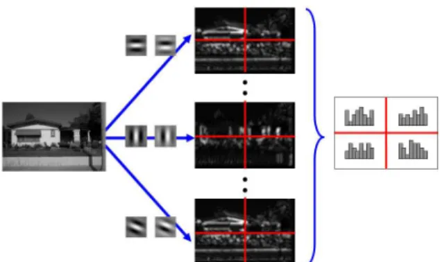
The proposed method consists of 3 steps. The first step extracts the features from images. In this paper, grid sampling with 16×16 grids is used, and orientation his-tograms of Gabor features are developed at each grid.
The second step is the local and global KPCAs. In local KPCA, 4 orientation histograms without position information on 2×2 grid are used as a local feature. In global KPCA, orientation histograms with topological information on an image are used. Local KPCA rep-resents the fine part of scenes and global KPCA repre-sents the rough composition of scenes. Note that global KPCA is position dependent and local KPCA is posi-tion independent. The third step is the classificaposi-tion by integrating the reconstruction errors in both KPCAs.
In section 2.1, orientation histogram of Gabor fea-tures is explained. Local and global KPCAs are ex-plained in section 2.2. Section 2.3 explains the classifi-cation by integration of both KPCAs.
2.1 Features for scene classification
In recent years, the effectiveness of orientation his-togram [1] for object recognition is reported. We de-velop the orientation histogram from multi-scale Gabor features because Gabor features are better representa-tion than simple gradient features [13].First, we define Gabor filters. They are defined as ψk(z) = k 2 ν σ2exp à −k2νzTz 2σ2 ! · ³ exp³ikTz´−exp³−σ2/2´´, (1) wherez= (y,x)T,k=kνexp(iφ) = (kνcos(φ),kνsin(φ))T,
kν =kmax/fν, φ =µ·π/8, f = √
2 and σ =π. In
Figure 1: Orientation histogram from Gabor features
the experiments, Gabor filters of 8 different orientations (µ={0, . . . ,7}) with 3 frequency levels (ν={0,1,2}) are used. In the following experiments, the norm of real and imaginary parts at each point is used as the output of a Gabor filter. The size of Gabor filters of 3 differ-ent frequency levels is set to 9×9, 13×13 and 17×17 pixels respectively.
Next, we explain how to develop the orientation his-togram from the output of Gabor filters. In this pa-per, the orientation histogram is developed from evenly sampledM×M grid. Figure 1 shows the example of 2×2 grid with only one scale parameter1. First, Gabor features (real and imaginary parts) of 8 orientations are extracted from the input image. The norm of real and imaginary parts at each pixel is computed. Then the ori-entation histogram with 8 bins at each grid is developed by voting the output value of the maximum orientation at each pixel to the orientation bin. This process is re-peated at each scale parameter independently.
In the experiments, we use evenly sampled 16×16 grid, and the orientation histogram of 24 dimensions (= 3 scales×8 orientation bins) is developed at each grid. Only 24 dimensional orientation histogram at each grid is too small to classify scenes by using only local features. Thus, we use 4 orientation histograms on 2×2 grid without overlap are used as one local fea-ture. Namely, 64 (= 8×8) local features are obtained from an image. The dimension of a local feature is 96 (= 24×2×2).
In local KPCA, local features without position infor-mation are used. In global KPCA, all 64 local features with position information are used.
2.2 Local and global KPCA with different
role
In this section, at first, we explain KPCA and kernel function. After that, local KPCA and global KPCA are explained.
Kernel PCA This section explains KPCA [16, 17] briefly. When data {x1. . . ,xL} is given, x is mapped 1In the experiments, Gabor features of 3 scale parameters are used. 2
into high dimensional space by non-linear mapping φ(x). By applying linear PCA in high dimensional space, non-linear principal components are obtained. Covariance matrix in high dimensional space is com-puted by C=1 L L
∑
i=1 φ(xi)φ(xi)T. (2) Eigen value problem for KPCA is defined byλV=CVwhereλ is eigen value andV are eigen vectors. Eigen vectors lie in the span ofφ(x1), . . . ,φ(xL). Therefore, the eigen vector is represented by
v=
∑
Li=1
αiφ(xi), (3) whereαiis the coefficient.
The equation does not change whenφ(xk)is multi-plied to both sides. Then the eigen value problem is changed as
λ φ(xk)TV=φ(xk)TCV for all k=1, . . . ,L. (4) By substituting eigen vectors shown in equation (3) into equation (4) and using the kernel matrixKwhere
Ki j=φ(xi)Tφ(xj), we obtain the following eigen value problem
Lλ α=Kα. (5) By solving the eigen value problem,α is obtained. We have to normalize the obtainedαpfor satisfyingvT
pvp= 1 for allp=1, . . . ,L.
An input samplexis mapped into the p-th principal component axis by vTpφ(x) = L
∑
i=1 αipK(xi,x). (6) The new feature vector in KPCA space is obtained by the weighted sum of similarities with training samples because kernel function computes the similarity with training samples.Next, moving on to consider the types of kernel func-tion, it is reported that a normalized polynomial kernel gives comparable performance with a Gaussian kernel using optimal parameters [18]. In addition, the param-eter dependency of a normalized polynomial kernel is much lower than that of a Gaussian kernel. Since a normalized kernel satisfies Mercer’s theorem [19], it is used as the kernel function. The normalized polynomial kernel is defined as
K(x,y) = φ(x)Tφ(y)
||φ(x)|| ||φ(y)||,
= p (1+xTy)d
(1+xTx)d(1+yTy)d. (7)
By normalizing the output of a standard polynomial kernel, the kernel value is between−1 and 1. In this paper, all orientation histograms are positive values as explained in section 2.1. Thus, the kernel value takes between 0 and 1 as with a Gaussian kernel. In local KPCA,d=5 is used empirically.
Local KPCA Since the distribution of local features without position information is non-linear, KPCA is appropriate for representing it [4, 20]. In this paper, KPCA is applied to the set of 4 orientation histograms without position information on 2×2 grid, and we call this “local KPCA”. Since the norm normalization of an input feature vector improves accuracy [6], the norm of each orientation histogram is normalized before apply-ing local KPCA.
Reconstruction error ofφ(x)by local KPCA can be computed as
||φ(x)−VVTφ(x)||2 = φ(x)Tφ(x)−φ(x)VVTφ(x) = K(x,x)− ||VTφ(x)||2. (8) Since we use a normalized polynomial kernel,K(x,x) =
1 and the reconstruction error takes the value between 0 and 1. ||VTφ(x)||2is called as CLAss-Featuring Infor-mation Compression (CLAFIC) [21, 22, 23, 24]. The reconstruction error is also called as Distance From Feature Space (DFFS) [25]. The reconstruction error
K(xi,xi)−||VTφ(xi)||2ofi-th local featurexiis denoted asεli.
In the classification by using only local KPCA, we compute the sum of reconstruction errors of all local features in an image, and the image is classified to the category which has minimum reconstruction error.
Global KPCA with local summation kernel In this paper, we want to compute the reconstruction error of the i-th local feature xi from local and global view-points, and both reconstruction errors are integrated to improve accuracy. When global KPCA without any de-vices is applied to the set of all local features of an im-age, we obtain only the total reconstruction errorεgand can not obtain the reconstruction error εgi of the i-th local feature xi. Therefore, we use the local summa-tion kernel [26] and the expansion of it [20] to compute the reconstruction error of i-th local feature by global KPCA.
Local summation kernel in which local kernels are summarized is defined as Ksum(x,y) = N
∑
i φ(xi)Tφ(yi) = N∑
i K(xi,yj) = φg(x)Tφg(y) (9) whereφg(x) = (φ(x1)T, . . . ,φ(xN)T)Tandx= (xT1, . . . ,xTN)T. Namely, in a local summation kernel, each local featurexiis mapped intoφ(xi)and global featureφg(x)is con-structed by connecting allφ(xi). After that linear PCA 3
is applied to the set ofφg(x)extracted from training im-ages.
If we use a normalized polynomial kernel with 2nd degree as a local kernel, we can compute eigen vectors of primal form directly not dual form. Therefore, we can compute the reconstruction error ofi-th local fea-ture by using the eigen vectors of the primal form. Note that dual form is the description using kernel function and primal form usesφ(x)directly not kernel function. In normalized polynomial kernel with 2nd degree (d=2 in equation (7)), the dimension of a mapped fea-tureφ(x)becomes(nd+2)(nd+1)/2 when the dimen-sion of an input featurexisnd. For example, the 2 di-mensional featurex= (x1,x2)Tis mapped into 6 dimen-sional feature φ(x) = (x2 1/a,x22/a, √ 2x1/a, √ 2x2/a, √
2x1x2/a,1/a)T where a is the norm of the vector
(x2 1,x22, √ 2x1, √ 2x2, √
2x1x2,1)T. Note that the norm of mapped feature is normalized to 1 in a normalized polynomial kernel. In this paper, the dimension ofφ(xi) is 4753 because the dimension of a local featurexiis 96. The eigen vectorsW with the primal form which are obtained by global KPCA with a local summation ker-nel can be described as
W= (w1, . . . ,wM), (10)
where M is the number of dimension (eigen vectors used) of KPCA space. The p-th eigen vectorwp can be described as
wp= (wTp1, . . . ,wTpN)T. (11)
This equation means that each eigen vector is con-nected the coefficient vectors forφ(xi)which is the fea-ture after non-linear mapping ofi-th local feature. The dimension ofwpicorresponds toφ(xi). Thus, a global feature xextracted from an image is mapped into the
p-th principal component axis as
wTpφg(x) = N
∑
i
wTpiφ(xi). (12) Since we use a local summation kernel, inner product between eigen vector andφg(x)can be decomposed into the summation of local inner products.
The difference from local KPCA is the eigen vectors which are determined by using entire feature extracted from an image. Namely, the eigen vectors of global KPCA are position dependent though the eigen vectors of local KPCA are not. Since global KPCA with a lo-cal summation kernel is the linear PCA ofφg(x), eigen vectors also have relative information with other local regions.
The computation of reconstruction error by global KPCA is easy becauseφg(x)andφdg(x) =WWTφg(x) can be computed directly by primal form. Since the to-tal reconstruction error||φg(xi)−φdg(xi)||2is the sum of
reconstruction error of all local features as∑Ni ||φ(xi)− d
φ(xi)||2, the reconstruction error of thei-th local feature can be computed easily. The reconstruction error ofi-th local feature is described asεgi.
In the classification by using only global KPCA, the total reconstruction error ∑Ni εgi of an image is com-puted, and the image is classified to the category which has minimum error.
2.3 Classification by inter-complementation
We integrate the reconstruction errors obtained by local and global KPCAs with different role. Figure 2 shows the reconstruction by local KPCA. Thei-th local fea-turexi(square region in the Figure) is mapped toφ(xi) which is shown as the circle in the Figure. The circle on the right side shows the reconstructed featureVVTφ(xi) by local KPCA. The difference between 2 circles is the reconstruction error ofi-th local feature.
Figure 3 shows the reconstruction by global KPCA with a local summation kernel. Thei-th local featurexi is mapped toφ(xi), and global feature is constructed as
φg(x) = (φ(x1)T, . . . ,φ(xN)T)T. The circle on the left side in the Figure shows the global featureφg(x)and the circle on the right side shows the reconstructed fea-tureWWTφg(x)by global KPCA. As shown in previous section, the total reconstruction error by global KPCA is divided into the reconstruction error at each local fea-ture.
The difference between the reconstruction error by local and global KPCAs is whether position dependent or not. In addition, global KPCA with a local summa-tion kernel uses the relasumma-tion with various regions though relative information with other regions is not used in local KPCA. Therefore, the integration of both recon-struction errors obtained from the different points of view will improve the accuracy.
To integrate the both reconstruction errors, we use the weighted integration as E=γ N
∑
i εli+ (1−γ) N∑
i εgi, (13) whereγ is the weight. A test image is classified to the category which gives the minimum integration error. If we setγto 0, the method corresponds to the use of only global KPCA. γ =1 means that only local KPCA is used. Experiments demonstrate the effectiveness of our integration method.3 EXPERIMENTS
In this section, the proposed method is evaluated us-ing the 13 scene database [15]. First, image database, evaluation method is explained in section 3.1. Next, evaluation results are shown in section 3.2.
Figure 2: Reconstruction by local KPCA
Figure 3: Reconstruction by global KPCA
3.1 Image database and evaluation method
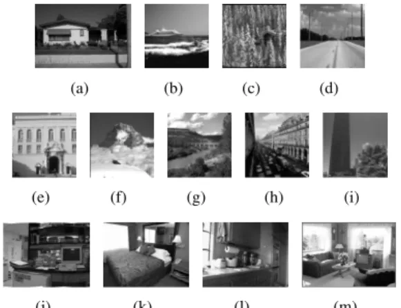
We use the database of 13 scene categories in order to compare our method with conventional studies [11, 12, 2, 13, 14]. The database includes only gray-level im-ages with various sizes. Each scene category has dif-ferent number of images. Examples of 13 scene cate-gories are shown in Figure 4. There are various scene categories such as outdoor and indoor. The within-class variance in scene classification is larger than that in face recognition problem because camera angle and objects in images are not static.In this paper, the images of each scene category are divided into two sets; training and test sets. 100 images selected randomly are used as training set. The remain-ing images of each scene category are used as test set. This protocol is the same as [11, 12, 2, 13, 14].
Each scene category has the different number of test images. The minimum and maximum number of test image of a class is 110 and 310. To reduce the bias of different number of test images, the mean of the clas-sification rate of each scene category is used in evalu-ation. This is also the same as conventional methods. We repeat this evaluation 3 times with different initial seed of a random function, and the mean classification rate of 3 runs is used as a final result.
3.2 Evaluation results
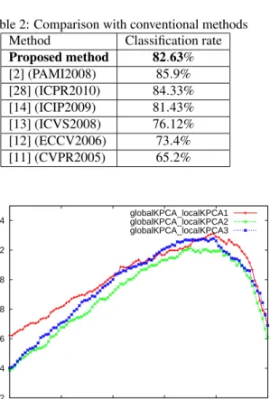
First, the proposed integration method is evaluated while changing the weightγin equation (13). Figure 5 shows the result in which horizontal axis isγ and the vertical axis is the correct classification rate. Note thatγ =0 means the use of only global KPCA andγ=1 means the use of only local KPCA. The 3 lines in the Figure
(a) (b) (c) (d)
(e) (f) (g) (h) (i)
(j) (k) (l) (m)
Figure 4: Examples of 13 scene images. (a) suburb (b) coast (c) forest (d) highway (e) inside-city (f) mountain (g) open-country (h) street (i) tall-building (j) office (k) bedroom (l) kitchen (m) living-room
mean the results with 3 different initial seeds for ran-dom function. The average classification rate of 3 runs is shown in Figure 6. Figures demonstrates that the in-tegration of 2 KPCAs with different role improves ac-curacy. The best accuracy achieves more than 82.5% though the accuracy of only local KPCA or global KPCA is below 77%. Namely, about 6% in accuracy is improved by very simple weighted integration.
Table 1 shows that best accuracy of the proposed method, the accuracy of only local and global KPCA. The best accuracy of the weighted integration method is obtained atγ=0.79. To show the baseline accuracy, we also evaluate the linear SVM of bag-of-visual words [27] which are commonly used in scene classification and object categorization. The basic feature for com-puting the visual words is 4 orientation histograms on 2×2 grid which are same as the proposed method. Ta-ble 1 also shows the accuracy. It achieves below 73%. This result shows the effectiveness of our method.
Finally, our method is compared with the conven-tional methods using the same database [11, 12, 13, 14, 2]. In general, the classification accuracy depends on the features and classifiers. Since each conventional method used different features and classifiers, the direct comparison with our method is difficult. Comparison result is shown Table 2. Note that accuracy of conven-tional methods is obtained from each paper. Since two methods [11, 12] used the bag-of-visual words with the local parts obtained from evenly sampled grid, they are similar with linear SVM of bag-of-visual words imple-mented by us. In [13], orientation histograms were de-veloped from subregions with various sizes. Our simple approach gives much better accuracy than the method. In [14], auto-correlation in KPCA space of visual words is used to give shift-invariance and relative informa-tion with neighboring regions to feature. The proposed method integrates the shift-invariance similarity by lo-5
Table 1: Evaluation result
Method Classification rate
Proposed method 82.63%
local KPCA 76.62%
global KPCA 74.71%
linear SVM of bag-of-words 72.66%
Table 2: Comparison with conventional methods Method Classification rate
Proposed method 82.63% [2] (PAMI2008) 85.9% [28] (ICPR2010) 84.33% [14] (ICIP2009) 81.43% [13] (ICVS2008) 76.12% [12] (ECCV2006) 73.4% [11] (CVPR2005) 65.2% 0.72 0.74 0.76 0.78 0.8 0.82 0.84 0 0.2 0.4 0.6 0.8 1 globalKPCA_localKPCA1 globalKPCA_localKPCA2 globalKPCA_localKPCA3
Figure 5: Accuracy of the proposed integration method
cal KPCA and the similarity with position dependent rough composition by global KPCA. Our simple ap-proach outperforms the result in [14]. Unfortunately, our method is worse than the method [2] using spatial pyramid probabilistic Latent Semantic Analysis and the method [28] using local co-occurrence features. How-ever, those methods used many devices while the pro-posed method is very simple in which the reconstruc-tion errors of 2 KPCAs are integrated by only one pa-rameter. In addition, the simple integration method is comparable to conventional methods though the direct comparison is difficult because of different features and classifiers. This shows the possibility of our approach. The accuracy will be improved further if we extend the proposed approach. This is a subject of future works.
0.74 0.75 0.76 0.77 0.78 0.79 0.8 0.81 0.82 0.83 0 0.2 0.4 0.6 0.8 1
Figure 6: Average accuracy of 3runs
4 CONCLUSIONS AND FUTURE WORKS
We proposed a scene classification method using the integration of rough composition by global KPCA and fine part by local KPCA. By giving the obvious differ-ent role to both KPCAs, the simple weighted integra-tion improved about 6% in comparison with only local and global KPCAs. The proposed method also outper-formed the linear SVM of bag-of-visual words with the same features. Our very simple approach gave com-parable accuracy with conventional methods using the same database. This shows the possibility of our ap-proach.In this paper, the simple weighted integration is used, and the accuracy is evaluated with the fixed weight for all test samples. However, if we select the appropri-ate weight for each test sample, the accuracy will be improved further. We may use the particle filter to se-lect the weight such as [4]. This is a subject for future works.
REFERENCES
[1] D. Lowe, “Distinctive image features from scale-invariant keypoints,” International Journal of Computer Vision60(2), pp. 91–110, 2004. [2] A. Bosch, A. Zisserman, and X. Munoz,
“Scene classification using a hybrid genera-tive/discriminative approach,” IEEE Trans. Pat-tern Analysis and Machine Intelligence 30(4), pp. 712–727, 2008.
[3] L. Fei-Fei, R. Fergus, and P. Perona, “Learning generative visual models from few training exam-ples: An incremental bayesian approach tested on 101 object categories,” inProc. CVPR Workshop of Generative Model Based Vision, 2004.
[4] K. Hotta, “Pose independent classifcation from small number of training samples based on kernel principal component analysis of local parts,”
age and Vision Computing27(9), pp. 1240–1251, 2009.
[5] A. Li, S. Shan, X. Chen, and W. Gao, “Maxmizing intra-indivisual correlations for face recognition across pose differences,” inProc. IEEE CS Con-ference on Computer Vision and Pattern Recogni-tion, 2009.
[6] K. Hotta, “Local normalized linear summation kernel for fast and robust recognition,” Pattern Recognition43(3), pp. 906–913, 2010.
[7] K. Hotta, “View independent face detection based on horizontal rectangular features and accuracy improvement using combination kernel of various sizes,” Pattern Recognition 42(3), pp. 437–444, 2009.
[8] R. P. N. Rao and D. H. Ballard, “Efficient encod-ing of natural time varyencod-ing images produces ori-ented space-time receptive fields,” tech. rep., 97.4, Dept of Comp Sci, Univ of Rochester, 1997. [9] K. Murphy, A. Torralba, D. Eaton, and W.
Free-man, “Object detection and localization using lo-cal and global features,” in Toward Category-Level Object Recognition, pp. 382–400, 2006. [10] T. Ishihara, K. Hotta, and H. Takahashi,
“Es-timation of object position based on color and shape contextual information,” inProc. Interna-tional Conference on Image Analysis and Process-ing, LNCS Vol.5716, pp. 57–62, 2009.
[11] L. Fei-Fei and P. Perona, “A bayesian hierarchi-cal model for learning natural scene categories,” inProc. IEEE CS Conference on Computer Vision and Pattern Recognition, pp. 524–531, 2005. [12] A. Bosch, A. Zisserman, and X. Munoz, “Scene
classification via plsa,” in Proc. 9th European Conference on Computer Vision, pp. 517–530, 2006.
[13] K. Hotta, “Scene classification based on multi-resolution orientation histogram of gabor fea-tures,” inProc. International Conference on Com-puter Vision Systems, LNCS Vol.5008, pp. 291– 301, 2008.
[14] K. Hotta, “Scene classification based on local au-tocorrelation of similarities with subspaces,” in
Proc. IEEE International Conference on Image Processing, pp. 2053–2056, 2009.
[15] 13 Scene categories database. http://vision.cs.princeton.edu/ Datab-sets/SceneClass13.rar.
[16] K.-R. Müller, S. Mika, G. Rätsch, K. Tsuda, and B. Schölkopf, “An introduction to kernel-based learning algorithms,” IEEE Trans. Neural Net-works12(2), pp. 181–201, 2001.
[17] B. Schölkopf, C. Burges, and A. Smola,Advances
in kernel methods: support vector learning, MIT Press, 1998.
[18] R. Debnath and H. Takahashi, “Kernel selection for the support vector machine,” IEICE Trans. Info. & Syst.E87-D(12), pp. 2903–2904, 2004. [19] J. Shawe-Taylor and N. Cristianini,Kernel
Meth-ods for Pattern Analysis, Cambridge University Press, 2004.
[20] K. Hotta, “Non-linear feature extraction by linear principal component analysis using local kernel,”
Pattern Recognition Recent Advances, pp. 99– 109, 2010.
[21] T. Balachander and R. Kothari, “Kernel based subspace pattern classification,” in Proc. Inter-national Joint Conference on Neural Networks, vol. 5, pp. 3119–3122, 1999.
[22] E. Oja,Subspace Methods of Pattern Recognition, Research Studies Press Ltd., 1983.
[23] S. Watanabe,Knowing and Guessing - Quantita-tive Study of Inference and Information, John Wi-ley & Sons, 1969.
[24] S. Watanabe and N.Pakvasa, “Subspace method of pattern recognition,” inProc. 1st International Joint Conference on Pattern Recognition, pp. 25– 32, 1973.
[25] B. Moghaddam and A. Pentland, “Probabilistic visual learning for object representation,” IEEE Trans. Pattern Analysis and Machine Intelligence
19(7), pp. 696–710, 1997.
[26] K. Hotta, “Robust face recognition under partial occlusion based on support vector machine with local gaussian summation kernel,”Image and Vi-sion Computing26(11), pp. 1490–1498, 2008. [27] G. Csurka, C. Dance, L. Fan, J. Willamowski, and
C. Bray, “Visual categoraization with bags of key-points,” inProc. ECCV Workshop on Statistical Learning in Computer Vision, pp. 1–16, 2004. [28] K. Hotta, “Scene classification using local
co-occurrence feature in subspace obtained by kpca of local blob visual words,” inProc. International Conference on Pattern Recognition, pp. 4230– 4233, 2010.