©
DOI: 10.1534/genetics.104.033373
A Genetic Interpretation of the Variation in Inbreeding Depression
Jacob A. Moorad
1and Michael J. Wade
Department of Biology, Indiana University, Bloomington, Indiana 47405
Manuscript received July 13, 2004 Accepted for publication April 12, 2005
ABSTRACT
Inbreeding depression is expected to play an important but complicated role in evolution. If we are to understand the evolution of inbreeding depression (i.e., purging), we need quantitative genetic interpreta-tions of its variation. We introduce an experimental design in which sires are mated to multiple dams, some of which are unrelated to the sire but others are genetically related owing to an arbitrary number of prior generations of selfing or sib-mating. In this way we introduce the concept of “inbreeding depression effect variance,” a parameter more relevant to selection and the purging of inbreeding depression than previous measures. We develop an approach for interpreting the genetic basis of the variation in inbreeding depression by: (1) predicting the variation in inbreeding depression given arbitrary initial genetic variance and (2) estimating genetic variance components given half-sib covariances estimated by our experimental design. As quantitative predictions of selection depend upon understanding genetic variation, our approach reveals the important difference between how inbreeding depression is measured experimentally and how it is viewed by selection.
W
HEN populations experience inbreeding, mean Variation in ID (2ID) has been measured as part of studies investigating the relationship between ID and fitness tends to decline and the among-line
vari-ance in mean fitness increases (Darwin 1877, p. 442; mating system (e.g.,Kalisz1989;AgrenandSchemske
Morton et al. 1956; Charlesworth and Charles- 1993;MutikainenandDelph1998;Takebayashiand
worth 1987; Byers and Waller 1999). Inbreeding Delph2000; reviewed inByersandWaller1999) and
increases homozygosity, causing a decline in mean fit- between ID and the short-term dynamics of purging ness owing to the manifestation of recessive deleterious (PrayandGoodnight1995;Fowler andWhitlock alleles, the reduction in frequency of heterozygotes at 1999). In these latter studies, ID is considered a herita-overdominant loci, or changes in gene interactions, ble trait and2IDis assumed to represent an opportunity such as additive-by-dominance and dominance-by-domi- for selection to act upon and reduce inbreeding load. nance epistasis (Crow and Kimura1970, pp. 78–80). The problem with this perspective is that inbreeding The among-line variance also increases owing to the seg- complicates the concept of heritability by changing the regation among lines of these genetic factors as well as nature of the regression of parents on offspring. Indeed, the additive and additive-by-additive epistatic genetic vari- Falconer (1985, p. 337) states that the concept of ances (CockerhamandWeir1968;Goodnight1988). breeding value, from which narrow sense heritability Inbreeding depression (ID) is believed to play an is measured, has “no useful meaning when mating is important but complicated role in the evolution of mat- nonrandom.” Although the change in the parent-off-ing systems (e.g., Holsinger 1988; Uyenoyama et al. spring regression can be predicted for particular cases 1993). For example, in the evolution of selfing and (e.g., for selfing, see Wright and Cockerham1986), outcrossing in plants, inbreeding initially selects against the variance components affecting selective response in selfing lineages by lowering mean fitness. However, if inbred populations are different from those contribut-the genes responsible for ID are purged by selection ing to2
ID.
from within or among some lineages, then the selective The response to selection with inbreeding has been advantages of selfing may come to outweigh its initial addressed by a large body of theory describing trait disadvantages. The purging process is complicated be- variation among lineswith inbreeding or the within-line cause inbreeding has effects not only on mean fitness covariance among traits with inbreeding (e.g., Cocker-but also on the within-deme genetic variances and co- ham1971, 1983;CorneliusandDudley1976; Cocker-variances of fitness traits. Thus, purging of ID depends hamandWeir1983, 1984;CockerhamandMatzinger upon the within- and among-line genetic variances. 1985;WrightandCockerham1986;Cornelius1988).
Kelly (2004) noted that 2
ID includes several within-family covariances, e.g., the covariances between out-1Corresponding author:Department of Biology, Indiana University,
bred relatives, between outbred and inbred relatives, Jordan Hall, 1001 E. 3rd St., Bloomington, IN 47405-7005.
E-mail: [email protected] and between inbred relatives. However, only the
Figure 1.—Lineage-spe-cific inbreeding depression with selfing and sib-mating. (A) Each selfing line begins with an outbred hermaphro-dite at generation 0. Follow-ingg ⫺1 consecutive gen-erations of selfing in which a single hermaphrodite is se-lected for crossing, a sire is simultaneously crossed to
Mooutbred and unrelated fe-males and to itself (the sire is the dam used to generate inbred progeny in genera-tiong). With this design, re-lated dam replication is not possible with selfing (the sire must be the dam for selfing to occur). (B) Each sib-mating line begins with two outbred and unrelated individuals at generation 0. Followingg⫺1 consecutive generations of sib-mating in which a single pair of siblings is selected for crossing, a sire is simultaneously crossed toMo outbred and unrelated females andMfsisters. The most recent ancestors through which inbred individuals may be made identical by descent are indicated by an asterisk. With selfing, this designation is given to only the sire. With sib-mating, it is given to both paternal grandparents (generationg⫺2).
ance between inbred relatives contributes to the among- tively understand the evolution of ID we need genetic variance estimates. In this way, the translation of the line variance in the inbred phenotype. This distinction
arises because ID is a group-level phenotype, defined variation in inbreeding depression into genetic variance components serves two purposes. The first is interpreta-as adifferencebetween inbred and outbred mean
pheno-types. The ID of an individual’s progeny depends upon tive: we may use the variation in inbreeding depression as a quantitative tool with which to estimate variance its own genotype as well as that of its mates. As a result,
selection among individuals in an inbreeding popula- components. The second is predictive: by understand-ing how genetic variation generates variation in inbreed-tion may not have a commensurate effect on ID.
Differ-ently put, trait evolution with inbreeding is different ing depression, we may predict future2
IDafter selection and/or inbreeding.
from the evolution of inbreeding depression.
This is not to say that inbreeding depression cannot In this article, we develop a general quantitative ge-netic framework for evaluating the gege-netic causes of evolve. However, a quantitative genetic model for the
evolution of ID requires refinements to our current 2ID. Because the evolution of mating systems depends upon the trade-off between kinship and ID, the develop-understanding of the genetic basis of ID. First, estimates
of ID appropriate for predicting a response to selection ment of this theory is a necessary step in the quantitative study of the evolution of mating systems. Specifically, must be made. For example, within-line replication of
mates is critical for quantifying the genetic variation we introduce an experimental design (Figure 1) for analyzing the genetic components ofID2 , when inbreed-available for mitigating inbreeding depression.
Never-theless, within-line mate replication is seldom (if ever) ing is caused by either selfing or sib-mating. Our ap-proach is a half-sib design, with sires mated to groups employed in practice.LynchandWalsh(1998, p. 268)
recommend that experimenters consider a replicated of related and unrelated dams. It permits ID to be de-fined for each sire as the difference between outbred nonrandom mating system (i.e., inbreeding) in the
con-text of similarly replicated panmixia: “A central problem and inbred dam means and addresses the need identi-fied byLynchandWalsh(1998, pp. 268–269) for an
is that inbreeding depression is not just a property of the
indi-vidual, but of the prospective mates as well . . . the fitness of ANOVA-based procedure for estimating the expected variation in ID : “. . . [genetic] variance in inbreeding de-progeny from full-sib matings will depend upon which sibs are
employed as mates. . .” and “. . .one would like an estimate of pression can [presumably] be estimated using ANOVA ap-proaches, treating differences between replicate pairs of inbred the fitness of outcrossed progeny averaged over all potential
mates. . . .” We argue that replication of mates is essen- and outcrossed matings within lineages as the units of observa-tions, but the procedures remain to be worked out.” We show tial for assessing evolutionarily relevant variation in
inbreeding depression, just as it is in experiments for that2IDconsists of predictable components of genetic variance and is sensitive to type and duration of inbreed-estimating variation in breeding values. To assess the
variation in inbreeding depression, we propose a modi- ing. The variation in inbreeding depression can be caused by varying F, the probability of identity by de-fication to the classic paternal half-sib design.
Parent-offspring regressions require estimates of com- scent, across lines. As we consider a design with invariant
quantita-differences, we find the total variation in inbreeding
depres-TABLE 1
sion across sires. This willoverestimatethe variation in
inbreed-Genetic effects on phenotypes ing depression effects because there will be contributions from
dam and individual (error) effects. Replication at the level of
Symbol Parameter dam (related and unrelated) and the offspring (inbred and
outbred) within each line provides a statistical means for ac- Mean of outbred and inbred populations counting for the extraneous variance components and
allow-b Mean inbreeding depression ing for unbiased estimates of2
IDE. If there areNsires,Mo
un-sio Effect of sireiwhen crossed to unrelated dams related dams,Mfrelated dams,nooutbred offspring, andnf
sif Effect of sireiwhen crossed to related dams inbred offspring, then
diok Effect of damkwhen crossed to unrelated sirei
difk Effect of damkwhen crossed to related sirei 2(zio..⫺zif..)⫽ 2 IDE⫹
1
Mo 2
do⫹
1
Mf 2
df⫹
1
noMo 2
eo⫹
1
nfMf 2
ef.
eiokl Deviation of individuall from the mean of cross
(4) sireiby unrelated damk
eifkl Deviation of individuall from the mean of cross The variance in inbreeding depression effectswithdam effect sireiby related damk variance has been measured in some experiments that do not
replicate at the level of the dam (e.g.,PrayandGoodnight
1995). This parameter contains variance components not rele-vant to a response to selection. We remove these components MATERIALS AND METHODS
by running two separate analyses of variances (ANOVAs) on the outbred and inbred individuals. Each is a two-factor ANOVA
The linear model:ConsiderNindependent lines, each
con-with random dam effects nested con-within random sire effects. taining one sire crossed toMfrelated females andMo
unre-This is different from previous approaches (Johnstonand lated and random-mated females. Each cross generatesno
out-Schoen1994;PrayandGoodnight1995) in which inbreed-bred offspring or nf inbred offspring (Figure 1). Let ziokl
ing level has been treated as a fixed effect. This alteration is represent the value of the phenotype of thelth outbred
indi-desirable asKelly(2004) points out that change in genetic vidual from the cross between theith sire and thekthunrelated
variation with inbreeding will violate the assumptions of homo-dam and, similarly,zifklrepresent the value of the phenotype
scedasticity upon which these early ANOVAs depend. Our dual-for an inbred offspring from the same sire but thekthrelated
ANOVA approach makes no such assumption. Note that there dam. We can decompose the phenotype of each outbred (o)
are no shared aspects between the outbred and inbred individ-and inbred (f ) individual into fixed individ-and rindivid-andom effects,
ualsexceptfor common alleles transmitted through the shared
ziok l⫽ ⫹1⁄2b⫹sio⫹doi k⫹eiok l and zifk l⫽ ⫺1⁄2b⫹sif⫹dfi k⫹eifk l, sires. Because the resulting covariance between outbred and (1) inbred sire effects is a desired component of2
IDE(Equation 3), no sort of joint ANOVA is more appropriate than the dual-where the terms in Equation 1 are defined in Table 1. We
ANOVA approach. define inbreeding depression for some sireito be the
expecta-tion of the phenotypic difference between outbred progeny
io .. and inbred progenyif .., or in terms of genetic effects,
RESULTS IDi⫽E((zio..⫺zif..)|si)⫽b⫹sio⫺sif. (2)
Interpretation of variance:Interpretations of the
pa-Since we are interested in the variation in the differential
effectsof inbreeding across breeding individuals, we define the rameters in Equation 4 are given in terms of genetic
variation ininbreeding depression effects(IDE),i.e., those trans- components described in Table 2. The variance terms
mitted by sires, to be in the ANOVAs can be expressed in terms of covariances
between relatives; these are affected by the type and
du-2
IDE⫽ 2(so)⫺2(so,sf)⫹ 2(sf). (3a)
ration of inbreeding. Each of these covariances can be
Sire effects are defined in part by the hypothetical
distribu-solved independently byCockerham(1971) for selfing
tion of paternal gametes across the entire population relevant
to that of the inbreeding treatment. Forsothis population is or byCockerham(1983) for sib-mating. Alternatively, the entire pool of unrelated individuals but forsfthis is only we may synthesize expressions that describe the appro-those individuals who share a specific type of relationship with priately weighted sums of these covariances and directly the sire. In the case of sib-mating, the sire’s gametes are
imag-yield the variance components used to estimate2 IDE. In ined to be combined with an infinite number of full sisters.
the appendix, we derive formulas for variation in
in-With selfing, however, the pool of appropriate mates is
re-stricted to the hermaphroditic sire itself. In this case, no mean- breeding depression effects as well as accessory variances
ingful distinction can be made between inbred sire effects (i.e., dam and error variances) in terms of genetic vari-and related dam effects (see Equation 4). This is reflected in ance components. These formulas are summarized in our definition for variation in inbreeding depression effects
Table 3. Variance components2
A,D1, andD*2 all have with selfing,
nonzero coefficients and contribute to2IDE. We show 2
IDE(selfing)⫽ 2(so)⫺2(so,sf)⫹ 2(sf)⫹ 2(df). (3b) below thatD
1andD*2 are often the predominant con-tributors to the variance in inbreeding depression. In
The terms2(s
f) and2(df) must be distinguished because the
latter contains genetic components and special environmental Table 4, we summarize the results for the first three components (maternal effects) not included in the former. generations of inbreeding and for inbreeding to
com-Adjusted estimator for the variance of inbreeding
depres-plete homozygosity. This illustrates the rate with which sion effects:The variation of inbreeding depression may be
the various components of variance change their
con-estimated by taking, for each sire, the mean outbred
TABLE 2
Definitions of genetic variance components
Genetic parameter General definition k⫽2
2
A: additive genetic variance 2兺ki⫽1pi␣2i 2p1p2(a⫺d(p1⫺p2)*)2
D1: covariance between additive and 兺ki⫽1pi␣i␦ii 2p1p2(p1⫺p2)*(a⫺d(p1⫺p2)*)d homozygous dominance deviations
D*2: variance of homozygous dominance 兺k
i⫽1pi␦2ii⫺(兺ki⫽1pi␦ii)2 4p1p2(p31⫹p23⫺p1p2)d2 deviations
2
D: dominance variance 兺ki⫽1兺kj⫽1pipj␦2ij 4p21p22d2
H*: squared sum of homozygous (兺k
i⫽1pi␦ii)2 4p 2 1p
2 2d2 dominance deviations
Parameters are defined in terms of allelic frequencies (pi), additive effects (␣i), and dominance effects (␦ij) assigned tokarbitrary alleles segregating at a locus. Quantitative definitions followHarris(1964) and Cocker-ham(1983). Notation for the two-allele case followsFalconerandMackay(1996, p. 118) and describes ad-ditive effects (a) and dominance deviations in the heterozygote (d). We usep1to represent the frequency of the high-valued allele. We assume that this allele is dominant; otherwise the difference marked with * is reversed.
Expected magnitude of the variation in inbreeding ance, then the vector describing the components of
2
IDE can be approximated by three elements: 2A, D1,
depression effects at mutation-selection balance:If
ge-netic variation is maintained by mutation-selection bal- andD*2. This follows from Table 2, last column, where
TABLE 3
Genetic composition of variation in inbreeding depression forggenerations of inbreeding
Source of
Variance Selfing Sib-mating
Inbreeding depression effects
2 A
D1
D*2 2 D H* ⎛ ⎜ ⎜ ⎜ ⎜ ⎜ ⎝ 1⁄ 2 1⁄4
2 1⁄
2
1 1⁄
8
0 1⁄
4
0 1⁄
8 ⎞ ⎟ ⎟ ⎟ ⎟ ⎟ ⎠
· r⫺
⎛ ⎜ ⎜ ⎜ ⎜ ⎜ ⎝ 0 0 0 0 F2 ⎞ ⎟ ⎟ ⎟ ⎟ ⎟ ⎠ ⎛ ⎜ ⎜ ⎜ ⎜ ⎜ ⎝ 1⁄
2 1⁄4 5⁄16 3⁄16 5⁄16 3⁄16 1⁄4 3⁄16 1⁄8
2 1⁄
2 7⁄8 5⁄16 7⁄8 5⁄16 1⁄2 5⁄16 1⁄8
1 1⁄
8 23⁄64 5⁄64 23⁄64 5⁄64 3⁄16 7⁄64 1⁄32
0 1⁄
4 5⁄32 11⁄64 5⁄32 11⁄64 1⁄4 21⁄128 1⁄8
0 1⁄
8 3⁄64 1⁄16 3⁄64 1⁄16 1⁄16 5⁄128 1⁄32
⎞ ⎟ ⎟ ⎟ ⎟ ⎟ ⎠
· r⫺
⎛ ⎜ ⎜ ⎜ ⎜ ⎜ ⎝ 0 0 0 0 F2 ⎞ ⎟ ⎟ ⎟ ⎟ ⎟ ⎠ Source of
Variance Outbred Inbred Outbred Inbred
Dam
NA
2 A
D1
D*2 2 D H* ⎛ ⎜ ⎜ ⎜ ⎜ ⎜ ⎝ 1⁄ 4 1⁄4
0 0
0 0
1⁄ 2 1⁄4
0 0 ⎞ ⎟ ⎟ ⎟ ⎟ ⎟ ⎠ · r ⎛ ⎜ ⎜ ⎜ ⎜ ⎜ ⎝ 1⁄
4 1⁄4 1⁄4 1⁄4 1⁄4 1⁄4 1⁄4 1⁄4 1⁄4
0 0 0 0 0 0 0 0 0
0 0 0 0 0 0 0 0 0
1⁄
2 1⁄4 3⁄8 1⁄4 3⁄8 1⁄4 3⁄8 5⁄16 1⁄4
0 0 0 0 0 0 0 0 0
⎞ ⎟ ⎟ ⎟ ⎟ ⎟ ⎠ · r ⎛ ⎜ ⎜ ⎜ ⎜ ⎜ ⎝
0 0 1⁄
16 1⁄16 1⁄16 1⁄16 1⁄8 1⁄8 1⁄8
0 0 1⁄
8 1⁄16 1⁄8 1⁄16 1⁄4 3⁄16 1⁄8
0 0 3⁄
64 1⁄64 3⁄64 1⁄64 3⁄32 1⁄16 1⁄32
0 0 1⁄
32 3⁄64 1⁄32 3⁄64 1⁄16 5⁄64 3⁄32
0 0 ⫺1⁄
64 0 ⫺1⁄64 0 ⫺1⁄32 ⫺1⁄64 0
⎞ ⎟ ⎟ ⎟ ⎟ ⎟ ⎠ · r Error 2 A D1
D*2 2 D H* ⎛ ⎜ ⎜ ⎜ ⎜ ⎜ ⎝ 1⁄ 4 1⁄2
0 0
0 0
1⁄ 2 3⁄4
0 0 ⎞ ⎟ ⎟ ⎟ ⎟ ⎟ ⎠ · r ⎛ ⎜ ⎜ ⎜ ⎜ ⎜ ⎝
0 1⁄
2
0 1
0 3⁄
8
0 1⁄
4
0 ⫺1
⁄8 ⎞ ⎟ ⎟ ⎟ ⎟ ⎟ ⎠ · r ⎛ ⎜ ⎜ ⎜ ⎜ ⎜ ⎝ 1⁄
4 1⁄2 3⁄8 1⁄2 3⁄8 1⁄2 3⁄8 7⁄16 1⁄2
0 0 0 0 0 0 0 0 0
0 0 0 0 0 0 0 0 0
1⁄
2 3⁄4 5⁄8 3⁄4 5⁄8 3⁄4 5⁄8 11⁄16 3⁄4
0 0 0 0 0 0 0 0 0
⎞ ⎟ ⎟ ⎟ ⎟ ⎟ ⎠ · r ⎛ ⎜ ⎜ ⎜ ⎜ ⎜ ⎝
0 1⁄
2 1⁄4 1⁄2 1⁄4 1⁄2 1⁄4 3⁄8 1⁄2
0 1 1⁄
2 3⁄4 1⁄2 3⁄4 1⁄2 1⁄2 1⁄2
0 3⁄
8 7⁄32 9⁄32 7⁄32 9⁄32 7⁄32 13⁄64 3⁄16
0 1⁄
4 3⁄16 13⁄32 3⁄16 13⁄32 3⁄16 49⁄128 17⁄32
0 ⫺1
⁄8 ⫺1⁄32 ⫺1⁄16 ⫺1⁄32 ⫺1⁄16 ⫺1⁄32 ⫺3⁄128 ⫺1⁄32
⎞ ⎟ ⎟ ⎟ ⎟ ⎟ ⎠ · r
Variances matrices are simplified forms of Equations A3 and A5. The vectorrdescribes the relationship in Jacquard identity coefficients
(Table A1) between the most recent ancestors through which inbred individuals may be made identical by descent (Figure 1). The
vector isrgiven by Equations A1 for sib-mating and A4 for selfing.Fis the probability of identity by descent of inbred individuals and
can be obtained by Equation A2. Sire effects variances and covariance are not given separately in this table (although they may be
derived using Equation A2). Instead, they are pooled into a single matrix to give2
TABLE 4
Contributions to variation in ID forggenerations of consecutive inbreeding
Source of Selfing: Sib-mating:
variance g⫽(1 2 3 ∞) g⫽(1 2 3 ∞)
Inbreeding depression effects 2
A
D1
D*2 2 D H* ⎛ ⎜ ⎜ ⎜ ⎜ ⎜ ⎝ 1⁄
4 3⁄8 7⁄16 1⁄2 1⁄
2 5⁄4 13⁄8 2 1⁄
8 9⁄16 25⁄32 1 1⁄
4 1⁄8 1⁄16 0 ⫺1⁄
8 ⫺1⁄2 ⫺47⁄64 ⫺1 ⎞ ⎟ ⎟ ⎟ ⎟ ⎟ ⎠ ⎛ ⎜ ⎜ ⎜ ⎜ ⎜ ⎝ 1⁄
8 3⁄16 1⁄4 1⁄2 1⁄
8 5⁄16 19⁄32 2 1⁄
32 7⁄64 61⁄256 1 1⁄
8 45⁄256 351⁄2048 0 ⫺1⁄
32 ⫺25⁄256 ⫺415⁄2048 ⫺1 ⎞ ⎟ ⎟ ⎟ ⎟ ⎟ ⎠ Source of
variance Outbred Inbred Outbred Inbred
Dam
NA 2
A
D1
D*2 2 D H* ⎛ ⎜ ⎜ ⎜ ⎜ ⎜ ⎝ 1⁄
4 1⁄4 1⁄4 1⁄4
0 0 0 0
0 0 0 0
1⁄
4 3⁄8 7⁄16 1⁄2
0 0 0 0
⎞ ⎟ ⎟ ⎟ ⎟ ⎟ ⎠ ⎛ ⎜ ⎜ ⎜ ⎜ ⎜ ⎝ 1⁄
4 1⁄4 1⁄4 1⁄4
0 0 0 0
0 0 0 0
1⁄
4 5⁄16 11⁄32 1⁄2
0 0 0 0
⎞ ⎟ ⎟ ⎟ ⎟ ⎟ ⎠ ⎛ ⎜ ⎜ ⎜ ⎜ ⎜ ⎝ 1⁄
8 1⁄8 3⁄32 0 1⁄
8 3⁄16 5⁄32 0 1⁄
32 1⁄16 7⁄128 0 3⁄
32 5⁄64 7⁄128 0 0 ⫺1⁄64 ⫺1⁄64 0 ⎞ ⎟ ⎟ ⎟ ⎟ ⎟ ⎠ Error 2 A D1
D*2 2 D H* ⎛ ⎜ ⎜ ⎜ ⎜ ⎜ ⎝ 1⁄
2 3⁄8 5⁄16 1⁄4
0 0 0 0
0 0 0 0
3⁄
4 5⁄8 9⁄16 1⁄2
0 0 0 0
⎞ ⎟ ⎟ ⎟ ⎟ ⎟ ⎠ ⎛ ⎜ ⎜ ⎜ ⎜ ⎜ ⎝ 1⁄
2 1⁄4 1⁄8 0 1 1⁄
2 1⁄4 0 3⁄
8 3⁄16 3⁄32 0 1⁄
4 1⁄8 1⁄16 0 ⫺1⁄
8 ⫺1⁄16 ⫺1⁄32 0 ⎞ ⎟ ⎟ ⎟ ⎟ ⎟ ⎠ ⎛ ⎜ ⎜ ⎜ ⎜ ⎜ ⎝ 1⁄
2 7⁄16 13⁄32 1⁄4
0 0 0 0
0 0 0 0
3⁄
4 11⁄16 21⁄32 1⁄2
0 0 0 0
⎞ ⎟ ⎟ ⎟ ⎟ ⎟ ⎠ ⎛ ⎜ ⎜ ⎜ ⎜ ⎜ ⎝ 1⁄
2 3⁄8 5⁄16 0 1⁄
2 1⁄2 1⁄2 0 3⁄
16 13⁄64 53⁄256 0 17⁄
32 95⁄256 561⁄2048 0 ⫺1⁄
32 ⫺7⁄256 ⫺65⁄2048 0 ⎞ ⎟ ⎟ ⎟ ⎟ ⎟ ⎠
With selfing, inbred dam effects are included in2
IDE. Otherwise, dam effect variance coefficients are obtained by subtracting half-sib covariances from full-sibs covariances. Error variance coefficients are obtained by subtracting full-sib covariances from individuals’ covariance with themselves.
we see that these components are roughly proportional p2, with expectation in terms of mutational parameters to the frequency of the rare allele. In contrast, the re- and s, then we may approximate the variation in maining two components,2
DandH*, are proportional inbreeding depression effects by finding the con-to the square of that frequency and can be ignored. tribution of D*2. With one generation of inbreeding, When genetic variation is maintained by the balance from Equation 5 and Table 4, we find the variation in between mutation and purifying selection, we expect inbreeding depression effects to be
thatp2Ⰶ p1when the effects of allele 1 are dominant
to the effects of allele 2 (CharlesworthandCharles- 2
IDE(selfing)⬵ s
4 2
A and 2IDE(sibbing)⬵ s
16 2 A. worth1987). To predict 2IDE, we assume a per-locus
(6) mutation rate (), selective effect (s), and average
de-gree of dominance (h). Below, we express results for
Thus, with complete dominance we expect enormous the various variance components in terms of additive
variation in inbreeding depression effects relative to2A, genetic equivalents,i.e., in multiples of2Athat segregates
nearly all generated by nonadditive genetic variation. in a random-mated population.
Partial dominance:Following the arguments above, we
Complete dominance ( h⫽0 ) :FollowingFalconerand
can approximate the value of variance components for Mackay(1996, p. 126) and Table 2 with complete
domi-partial dominance with rare alleles: nance (i.e.,d⫽ a), we have proportional values,
D1⬵
d
(a⫺d) 2 A⫽
1⫺2h
2h
2
A and D*2 ⬵
(1⫺2h)2 2h2
2 A. D1⬵
1
p2 2
A and D*2 ⬵ 2
p22 2
A. (5)
(7) Although bothD1 and D*2 ⬎ 2A, D*2 ⰇD1 when p2 is
Equa-Figure2.—Important genetic components that contribute to the variation in inbreeding depression effects (assuming rare alleles). Increasing the number of consecutive generations of selfing or sib-mating (indicated by thex-axis) increases the total variation in inbreeding depression effects (given in units of additive genetic variance equivalents). This incremental change in 2
IDEdiminishes with more generations of inbreeding and more quickly with more intense inbreeding (selfing). Low values ofh (corresponding toincreaseddominance deviations in heterozygotes andincreasedmean inbreeding depression) give more inbreed-ing depression effect variance than do high values of h. Changes in2IDEwithhare positively associated with the relative con-tribution ofD*2 toward that variance. With lowh,D2*will tend to dominate2IDE, althoughD1will still have some effect. In this case, additive genetic variation does not meaningfully contribute to the variation in inbreeding depression effects. At high values ofh, all three variance components become relatively important.
tion 7 and Table 4, the variance in inbreeding depres- high dominance (h⫽0.1), additive genetic variation is never an important source of variation in inbreeding sion effects is
depression effects. The relative contributions of2A,D1, 2
IDE(selfing)⬵ 1 16h2
2
A and 2IDE(sibbing)⬵
1⫹4h2 64h2
2
A. andD*2 stabilize after a few generations of inbreeding.
Using variation in inbreeding depression to estimate (8)
genetic variance components:By contrasting the covari-Usingh ⫽0.1 (suggested by LynchandWalsh1998, ances between different sorts of relatives with selfing and p. 286, as representative of viability in Drosophila), we sib-mating, it is possible to estimate the genetic parame-expect2
IDEto equalⵑ62A(six additive genetic variance ters that contribute to variation in inbreeding popu-equivalents) after one generation of selfing and a little lations (Cornelius and Dudley 1976; Wright and
⬎3⁄
22Aafter one generation of sib-mating. If we reduce Cockerham1986). The inbreeding depression design dominance (h ⫽ 0.3), then 2
IDE decreases relative to illustrated in Figure 1 provides us with a convenient col-additive genetic variance (0.6942
TABLE 5
Dissection of genetic variance using elements of the variation in inbreeding depression effects for one generation of sib-mating
Half-sib covariances Linear combinations
Variance
components A B C 4A 4(2B⫺3A) 16(A⫺4B⫹2C)
2 A
D1
D*2 2
D
H*
⎛ ⎜ ⎜ ⎜ ⎜ ⎜ ⎝ 1⁄
4 0 0 0 0 ⎞ ⎟ ⎟ ⎟ ⎟ ⎟ ⎠
⎛ ⎜ ⎜ ⎜ ⎜ ⎜ ⎝ 3⁄
8 1⁄
8 0 0 0 ⎞ ⎟ ⎟ ⎟ ⎟ ⎟ ⎠
⎛ ⎜ ⎜ ⎜ ⎜ ⎜ ⎝
5⁄ 8 3⁄
8 1⁄
32 1⁄
8 ⫺1⁄ 32
⎞ ⎟ ⎟ ⎟ ⎟ ⎟ ⎠
⎛ ⎜ ⎜ ⎜ ⎜ ⎜ ⎝ 1 0 0 0 0 ⎞ ⎟ ⎟ ⎟ ⎟ ⎟ ⎠
⎛ ⎜ ⎜ ⎜ ⎜ ⎜ ⎝ 0 1 0 0 0 ⎞ ⎟ ⎟ ⎟ ⎟ ⎟ ⎠
⎛ ⎜ ⎜ ⎜ ⎜ ⎜ ⎝
0 0 1 4 ⫺1
⎞ ⎟ ⎟ ⎟ ⎟ ⎟ ⎠
Combinations of half-sib covariances (columnsA,B, andC) after one generation of sib-mating can be used to estimate genetic parameters. CovarianceAis the resemblance between outbred half-sibs,Bis that between outbred and inbred half-sibs, andCis that between inbred half-sibs. The three dominance parameters are not separable by this design (last column).
with one generation of sib-mating, half-sib covariances type. For example, LandeandSchemske(1985) mea-and useful linear combinations thereof are given in Ta- sure themean family-level inbreeding phenotype after ble 5. These can resolve additive genetic variance (by a a period of inbreeding to degreef, as␦ ⫽(zo⫺zf)/zo; conventional outbred paternal half-sib comparison), this is the mean of the individual values of relative in-the covariance between additive and dominance devi- breeding depression for each family. In contrast, like ations in homozygotes, and the dominance contribu- PrayandGoodnight(1995), we consider inbreeding tion toward among-line variance. As this design con- depression on an absolute scale,ID⫽ zo⫺ zf, and find siders only one degree of inbreeding (at a constantF), that variation in inbreeding depression is caused by the it cannot decouple dominance parametersD*2,2D, and stochastic segregation among sire lines of several ge-H* (WrightandCockerham1986) but in most cases netic effects, including additive genetic variation. Thus, (i.e., rare alleles) this composite estimate is dominated even in the absence of dominance, we can expect ID by D*2. Maximum-likelihood approaches are typically to vary among inbred lineages. Our analytical finding used to estimate variance components in inbred popu- agrees with that demonstrated in population genetic lations (e.g., Shaw et al.1998; Edwards andLamkey simulations bySchultz andWillis(1995). However, 2002;KellyandArathi2003) but these analyses are SchultzandWillis(1995), like many other theoreti-probably not necessary when the inbreeding designs are cal studies of mating-system evolution, use the
rela-balanced and not too complex. tive measure of inbreeding depression that has been
shown by Johnston and Schoen (1994) and Lynch andWalsh(1998, p. 268) to generate biased estimates
DISCUSSION
of mean inbreeding depression when estimated with By solving for probabilities specific to a given system limited numbers of offspring. We demonstrate below of inbreeding, variation in inbreeding depression can that even with an infinite number of offspring, the mean be described in terms of genetic variance components. and variance of such relative measures of inbreeding These variance components have been dealt with exten- depression are likely to be biased.
sively by several authors with varying forms of notation Consider the outbred and inbred family means, z o (seeWalshandLynch2000, p. 298;Kelly2004), often andz
f, and population means,zoandzf. Following the in the context of the joint effects of inbreeding and methods ofLynchandWalsh(1998, p. 818) for find-selection. These variance components may be estimated ing the expectation of a ratio,
by using linear combinations of the variance and covari-ance of inbred and outbred paternal half-sib, i.e., sire
冢
zo⫺zf zo冣
⬵
冢
zo⫺ zf zo冣
⫺ zf (zo)3
V(zo)⫹ 1 (zo)2
Cov(zo,zf) . effects. Because our model is general to the number of
inbred generations, the theory is predictive and testable. (9)
For example, if genetic variance components were
esti-Given our results above, we can quantify the bias of this mated after a single generation of sib-mating, the
magni-estimate for any case of regular inbreeding for the typi-tude of variation in inbreeding depression could be
cal experimental study of inbreeding depression in predicted for any subsequent generation.
plants conducted without replication of unrelated dams Usually lineage-specific inbreeding depression is
ad-ditive genetic variance, dominance variance, and the co- nance. Finally, provided that phenotypes are normally distributed within an inbreeding class (or in the outbred variance between additive and homozygous dominance
deviations contribute toward the bias in ratio estimates population), we expect that the distribution of inbreed-ing depression across sires is normally distributed with ofmeaninbreeding depression,
mean equal to the average of all IDi(Equation 2) and variance given in Equation 4. In contrast, Johnston
冢
zo⫺zfzo
冣
⫺
冢
zo⫺zfzo
冣
⬵zo⫺zf 2(zo)3
2 A⫺
zf 4(zo)3
2 D⫹
1 4(zo)2
D1.
andSchoen(1994) report skew for simulated distribu-(10) tions of inbreeding depression, a result they attribute to “nonlinear functions of self- and outcrossed values.” The estimate ofvariancein relative inbreeding
depres-Our Equations 10 and 13 model this nonlinearity for a sion is also biased. FollowingLynchandWalsh(1998,
single generation of selfing. For these reasons, we argue p. 818), mean inbreeding depression changes the way
that relative measures of inbreeding depression are of the variance is calculated:
dubious relevance to evolutionary genetics.
Intuitively, we expect that lineage-level selection would
2
冢
zo⫺zf zo冣
⬵2(zfzo⫺ zozf) (zo)4
. (11a)
operate on an absolute scale without regard for a relative measure of inbreeding depression. For example, lines By expanding the numerator, we see that changes in pop- that enjoy a fitness advantage when outbred (relative ulation means with inbreeding affect the relative weight- to other outbred lines)andan advantage when inbred ings of genetic variance components: (relative to other inbred lines) will have high fitness
regardless of the lines’ proportional inbreeding
depres-2
冢
zo⫺zf zo冣
⬵(zf)22(zo)⫺2(zf)(zo)(zo,zf)⫹(zo)22(zf) (zo)4
.
sion. Alternatively, a line that performs poorly regardless of mating system is unlikely to thrive despite little pro-(11b)
portional inbreeding depression. Lineage-specific fitness Because of the weights of variance and covariance com- depends upon the outbred phenotype, the inbred pheno-ponents on the right-hand side of Equation 11b, it is type, and the covariation between the two (weighted by not likely that the variation in proportional inbreeding the frequencies of the classes). Although not all absolute depression will closely resemble the variance of absolute measures of lineage-specific inbreeding depression (e.g., inbreeding depression. Again, we reconsider the case of PrayandGoodnight1995) are indicative of lineage-unreplicated dams and a single generation of selfing. specific fitness, they do have the advantage of providing From Table 4, we know that variation in inbreeding de- information from which to draw quantitative genetic in-pression taken on the absolute scale is independent of ferences as we have shown above. These inferences are
population means: important because they allow us to make quantitative
predictions regarding the response to selection with
in-2
ID(selfing,Mo⫽1)⫽ 2
IDE(selfing)⫹ 2(do)
breeding (Cornelius andDudley 1976; Cockerham
⫽1⁄ 2
2
A⫹1⁄2D1⫹1⁄8D*2 ⫹1⁄2 2
D⫺1⁄8H*. andMatzinger1985).
(12) Because of the genetic covariance between the out-bred and inout-bred phenotypes, inbreeding depression will On the relative scale, however, variation in inbreeding
evolve as a by-product of natural selection in an out-depression is confounded by population mean
pheno-breeding population, in the same way that hybrid invi-types (Equation 11b), specifically
ability between populations evolves as a by-product of local adaptation within populations. When the genetic
2
冢
zo⫺zfzo
冣
⬵(zo) ⫺4
冢冤
1⁄2(zf)2⫺(zf)(zo)⫹(zo)2
冥
2A.covariance is positive, selection within an outbreeding population will mitigate future inbreeding depression.
⫹(zo)[(zo)⫺1⁄2(zf)]D1 Conversely, the outbred phenotype evolves as a corre-lated response to selection within inbreeding
popula-⫹1⁄
8(zo)2D*2 ⫹1⁄4[(zf)2⫹(zo)2]2D
tions. When the genetic covariance is negative, selection
⫺1⁄
8(zo)2H*
冣
(13) within an inbreeding population could impede a later transition to outbreeding as a correlated response. Be-cause both2AandD1components exclusively contribute These relative genetic variance component weightings
are unbiased only when zo⫽ zf,i.e., when there is no to the covariance between outbred and inbred pheno-types andD1is positive with respect to fitness under the population inbreeding depression! Thus, the most
com-monly used experimental design yields biased estimates deleterious, recessive model of inbreeding depression, we expect the former: lineages that are good outcrossers of both the mean and the variance of inbreeding
depres-sion. Furthermore, the estimates contain components are good inbreeders.
Although inbreeding depression is often thought of of genetic variance irrelevant to the genetic causes of
domi-Cornelius, P. L., 1988 Properties of components of covariance of mal distribution of inbreeding depression effects, just
inbred relatives and their estimates in a maize population. Theor. as it will for any effect with a genetic basis and this dis- Appl. Genet.75:701–711.
Cornelius, P. L., andJ. W. Dudley, 1976 Genetic variance compo-tribution will have both a mean and a variance. Genetic
nents and predicted response to selection under selfing and full-models that translate the first moment of this
distribu-sib mating in a maize population. Crop Sci.16:333–339. tion (mean inbreeding depression) into mean genetic Crow, J. F., andM. Kimura, 1970 An Introduction to Population Genetics
Theory. Alpha Editions, Edina, MN. effects (e.g., additive effects, dominance effects, etc.) have
Darwin, C., 1877 Different Forms of Flowers of Plants of the Same Species. existed for the last half-century (Morton et al. 1956; J. Murray, London.
CrowandKimura1970;Lynch1991). These models Edwards, J. W., and K. R. Lamkey, 2002 Quantitative genetics of inbreeding in a synthetic maize population. Crop Sci.42:1094–1104. are useful for understandingextantpatterns of trait
val-Falconer, D. S., 1985 A note on Fisher’s ‘average effect’ and ‘aver-ues, such as assessing the relative dominance (or epistatic) age excess’. Genet. Res.46:337–347.
contributions toward some trait mean, but, because they Falconer, D. S., andT. F. C. Mackay, 1996 Introduction to Quantita-tive Genetics, Ed. 4. Longman Scientific & Technical, Harlow, UK. do not inform us as to the relationship between genetic
Fowler, K., andM. C. Whitlock, 1999 The variance in inbreeding variation and inbreeding depression, they are not ade- depression and the recovery of fitness in bottlenecked popula-quate for predicting response to selection (such as the tions. Proc. R. Soc. Ser. B266:2061–2066.
Goodnight, C. J., 1988 Epistasis and the effect of founder events mitigation of mean inbreeding depression by purging).
on the additive genetic variance. Evolution42:441–454. In contrast, theory that explicitly links genetic variation Harris, D. L., 1964 Genotypic covariance between inbred relatives. to selection with inbreeding is well developed (Corne- Genetics50:1319–1348.
Holsinger, K. E., 1988 Inbreeding depression doesn’t matter: The
lius and Dudley 1976; Cockerham and Matzinger
genetic basis of mating-system evolution. Evolution42:1235–1244. 1985;WrightandCockerham1986). The deficiency Jacquard, A., 1974 The Genetic Structure of Populations. Springer-Ver-in current Springer-Ver-inbreedSpringer-Ver-ing theory is that the observable varia- lag, New York.
Johnston, M. O., andD. Schoen, 1994 On the measurement of tion in inbreeding depression and the selectively
rele-inbreeding depression. Evolution48:1735–1741.
vant variation in genetic effects have not been recon- Kalisz, S., 1989 Fitness consequences of mating system, seed weight, and emergence date in a winter annual,Colinsia verna.Evolution ciled. In other words, measurements of the variance in
43:1263–1272. inbreeding depression have no quantitatively predictive
Kelly, J. K., 2004 Family level inbreeding depression and the evolu-value in regard to the response to selection with inbreed- tion of plant mating systems. New Phytol.165:55–62.
Kelly, J. K., andH. S. Arathi, 2003 Inbreeding and the genetic ing. Our ANOVA-based approach for inferring the
ge-variance of floral traits inMimulus guttatis.Heredity90:77–83. netic architecture of inbreeding depression from varia- Lande, R., andD. W. Schemske, 1985 The evolution of self-fertiliza-tion in inbreeding depression bridges the empirically tion and inbreeding depression. I. Genetic models. Evolution39:
24–40. measurable and the theoretically useful.
Lynch, M., 1991 The genetic interpretation of inbreeding depres-We thank John Kelly, Bruce Walsh, Elizabeth Housworth, and two sion and outbreeding depression. Evolution45:622–629.
Lynch, M., andJ. B. Walsh, 1998 Genetics and Analysis of Quantitative anonymous reviewers for comments on the article. This work was
Traits. Sinauer Associates, Sunderland, MA. supported by National Science Foundation grant DEB 0206628.
Morton, N. E., J. F. CrowandH. J. Muller, 1956 An estimate of the mutational damage in man from data on consanguineous marriages. Proc. Natl. Acad. Sci. USA42:855–863.
Mutikainen, P, andL. F. Delph, 1998 Inbreeding depression in LITERATURE CITED gynodioeciousLobelia siphilitica: among-family differences
over-ride between-morph differences. Evolution52:1572–1582.
Agren, J., andD. W. Schemske, 1993 Outcrossing rate and
inbreed-Pray, L. A., andC. J. Goodnight, 1995 Genetic variation in inbreed-ing depression in two annual monoecious herbs,Begonia hirsute
ing depression on the red flour beetleTribolium castaneum. Evolu-andB. semiovata.Evolution47:125–135.
tion49:176–188.
Byers, D. L., andD. M. Waller, 1999 Do plant populations purge
Schultz, S. T., andJ. H. Willis, 1995 Individual variation in in-their genetic load? Effects of population size and mating history
breeding depression: the roles of inbreeding history and muta-on inbreeding depressimuta-on. Annu. Rev. Ecol. Syst.30:479–513.
tion. Genetics141:1209–1223.
Charlesworth, D., andB. Charlesworth, 1987 Inbreeding
de-Shaw, R. G., D. L.Byersand F. H.Shaw, 1998 Genetic components pression and its evolutionary consequences. Annu. Rev. Ecol. Syst.
of variation inNemophila menziesiiundergoing inbreeding:
mor-18:237–268.
phology and flowering time. Genetics150:1649–1661.
Cockerham, C. C., 1971 Higher order probability functions of iden- Takebayashi, N., andL. F. Delph, 2000 An association between a tity of alleles by descent. Genetics69:235–246.
floral trait and inbreeding depression. Evolution54:840–846.
Cockerham, C. C., 1983 Covariances of relatives from self-fertiliza- Uyenoyama, M. K., K. E. HolsingerandD. M. Waller, 1993 Eco-tion. Crop Sci.23:1177–1180. logical and genetic factors directing the evolution of
self-ferti-Cockerham, C. C., andD. F. Matzinger, 1985 Selection response lization. Oxf. Surv. Evol. Biol.9:327–381.
based on selfed progenies. Crop Sci.25:483–488. Walsh, J. B., andM. Lynch, 2000 Evolution and Selection of
Quan-Cockerham, C. C., andB. S. Weir, 1968 Sib mating with two linked titative Traits(http://nitro.biosci.arizona.edu/zbook/volume_2/ loci. Genetics60:629–640. chapters/vol2_10.html).
Cockerham, C. C., andB. S. Weir, 1983 Variance in actual inbreed- Wright, A. J., andC. C. Cockerham, 1986 Covariances of relatives ing. Theor. Popul. Biol.23:85–109. and selection response in generations of selfing from an
out-Cockerham, C. C., andB. S. Weir, 1984 Covariances of relatives crossed base population. Theor. Appl. Genet.72:689–694. stemming from a population undergoing mixed self and random
APPENDIX
Sib-mating:The vectorrdescribes the relationship between the most recent common ancestral pair of all related inbred individuals of generationg(Figure 1, asterisks) in terms of Jacquard coefficients (Table A1). Note that all related outbred progeny are related to these grandparents through their common sire.
r⫽ ⎛ ⎜ ⎜ ⎜ ⎜ ⎜ ⎜ ⎜ ⎜ ⎜ ⎜ ⎝
1 0 1⁄
4 0 1⁄4 0 1⁄8 1⁄16 0
0 0 0 0 0 0 1⁄
8 0 0
0 0 1⁄
4 0 1⁄4 0 1⁄4 1⁄8 0
0 0 0 0 0 0 0 1⁄
16 0 0 0 1⁄
4 0 1⁄4 0 1⁄4 1⁄8 0
0 0 0 0 0 0 0 1⁄
16 0 0 1 1⁄
4 1⁄2 1⁄4 1⁄2 1⁄4 3⁄16 1⁄4 0 0 0 1⁄
2 0 1⁄2 0 3⁄8 1⁄2
0 0 0 0 0 0 0 0 1⁄
4
⎞ ⎟ ⎟ ⎟ ⎟ ⎟ ⎟ ⎟ ⎟ ⎟ ⎟ ⎠
g⫺2
· ⎛ ⎜ ⎜ ⎜ ⎜ ⎜ ⎜ ⎜ ⎜ ⎜ ⎜ ⎝ 0 0 0 0 0 0 0 0 1 ⎞ ⎟ ⎟ ⎟ ⎟ ⎟ ⎟ ⎟ ⎟ ⎟ ⎟ ⎠
. (A1)
This vector summarizes all inbreeding prior to generation g⫺ 2. This identity vector serves as a benchmark with which we generate a series of new identity vectors that describe all relationships within and between individuals of generationg. Five vectors correspond to siblings pairs: outbred full-sibs, v(OFS); outbred half-sibs,v(OHS); half-sibs in which one individual is outbred and the other is inbred,v(OF); the alternative,v(FO); inbred full-sibs,v(FFS); and inbred half-sibs,v(FHS). In addition, there are two vectors describing the resemblance within individuals: outbred individuals, v(O), and inbred individuals, v(F). All identity vectors for generationgcan be derived by taking the product ofrand the probability transition matrixAspecific to the type of relationship (given in Table A2).
Once we have the identity vectors for all siblings and individuals in generationg(the variousvvectors), we may translate them into variance components. For any v describing relativesi andj, the genetic covariance between them is (i,j)⫽T · v(i,j)⫺FiFjH* (Harris1964;Cockerham1971;Jacquard1974), where
T⫽
2 A D1 D*2 2
D H*
⎛ ⎜ ⎜ ⎜ ⎜ ⎜ ⎝
2 0 1 0 1 0 1 1⁄
2 0
4 0 1 0 1 0 0 0 0
1 0 0 0 0 0 0 0 0
0 0 0 0 0 0 1 0 0
0 1 0 0 0 0 0 0 0
⎞ ⎟ ⎟ ⎟ ⎟ ⎟ ⎠ and
Fi ⫽(1 1 1 1 0 0 0 0 0)· v, Fj⫽(1 1 0 0 1 1 0 0 0)· v. (A2)
Note that FiFj⬆ 0 if and only if both individuals are inbred. Because all inbred individuals are equally inbred in this design, we may defineFsuch thatF2⫽F
iFj.
We find sire, dam, and error effects variances for outbred and inbred cases by using combinations of these sibling and individual covariances. The sire effect variances are simply the half-sib covariances within outbred and inbred treatments. The covariance between outbred and inbred sire effects is the covariance between outbred and inbred half-sibs. The variation in inbreeding depression effects is a sum of these. Following from Equations 3a and A2,
2
IDE⫽T ·[A(OHS)⫺A(OF)⫺A(FO)⫹A(FHS)]· r⫺F2H*. (A3a)
Dam effect variances are the differences between full-sib and half-sib covariances. Outbred and inbred dam effect variances are
2(d
o)⫽T ·[A(OFS)⫺A(OHS)]· r and 2(df)⫽T ·[A(FFS)⫺A(FHS)]· r. (A3b)
Error variance (the within-full-sib family variation) is found by subtracting the full-sib covariance from the covariance of individuals with themselves. For outbred and inbred cases, these are
2(ε
o)⫽T ·[A(OP)⫺A(OFS)]· r and 2(εf)⫽T ·[A(FP)⫺A(FFS)]· r. (A3c)
All effect variances and covariances are simplified and summarized in Table 3.
TABLE A1
Jacquard’s condensed identity coefficients
Jacquard coefficient Probability that for individualsiandj
⌬1 i1⫽i2⫽j1⫽j2 ⌬2 i1⫽i2⬆j1⫽j2
⌬3 i1⫽i2⫽j1⬆j2ori1⫽i2⫽j2⬆j1 ⌬4 j2⬆i1⫽i2⬆j1andj1⬆j2
⌬5 i1⬆i2⫽j1⫽j2ori2⬆i1⫽j1⫽j2 ⌬6 i2⬆j1⫽j2⬆i1andi1⬆i2 ⌬7 i1⫽j1⬆i2⫽j2ori1⫽j2⬆j1⫽i2
⌬8 Identity is shared betweeniandjthrough only one pair of alleles
⌬9 No identity is shared between any alleles ofiandj
r⫽1 7 ⎛ ⎜ ⎝
1 1⁄ 2 0 1⁄
2
⎞ ⎟ ⎠
g⫺1
· ⎛ ⎜ ⎝ 0 1 ⎞ ⎟
⎠. (A4)
As with sib-mating, we use this vector to generate identity vectors for all relationships within and between individuals of generationg. Because there is only one inbred family per sire, there are no inbred half-sibs. Consequently, we
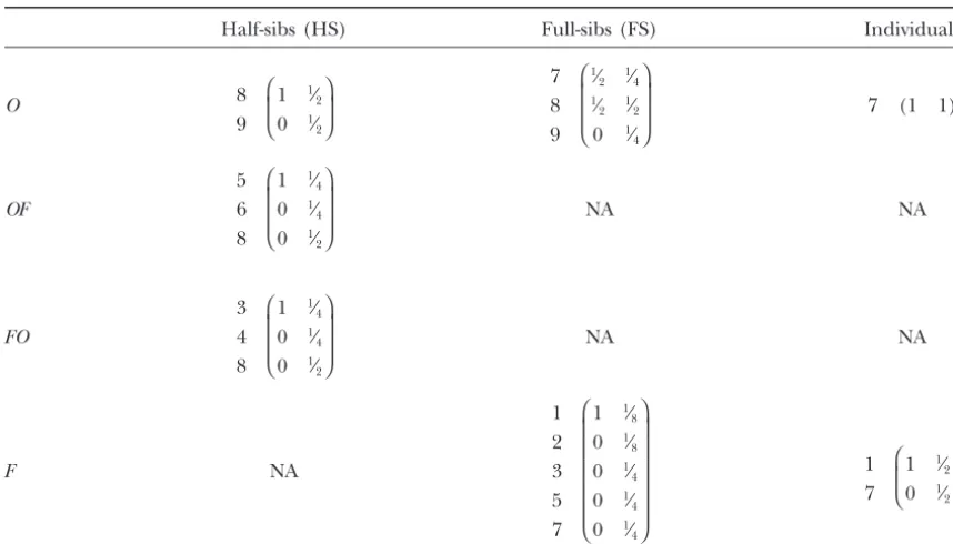
TABLE A2
Probability transition matrices (A) used to derive identity of relatives of generationg after an arbitrary number of sib-mated generations
Half-sibs (HS) Full-sibs (FS) Individuals (P)
O 8 7 (1 1 1 1 1 1 1 1 1)
9 ⎛ ⎜ ⎝
1 1⁄
2 3⁄4 1⁄2 3⁄4 1⁄2 3⁄4 5⁄8 1⁄2
0 1⁄
2 1⁄4 1⁄2 1⁄4 1⁄2 1⁄4 3⁄8 1⁄2
⎞ ⎟ ⎠
7 8 9
⎛ ⎜ ⎜ ⎝
1⁄
2 1⁄4 3⁄8 1⁄4 3⁄8 1⁄4 3⁄8 5⁄16 1⁄4 1⁄
2 1⁄2 1⁄2 1⁄2 1⁄2 1⁄2 1⁄2 1⁄2 1⁄2
0 1⁄
4 1⁄8 1⁄4 1⁄8 1⁄4 1⁄8 3⁄16 1⁄4
⎞ ⎟ ⎟ ⎠
OF NA NA
5 6 8 9
⎛ ⎜ ⎜ ⎜ ⎜ ⎝
1 1⁄
4 1⁄2 3⁄16 1⁄2 3⁄16 3⁄8 1⁄4 1⁄8
0 1⁄
4 1⁄8 3⁄16 1⁄8 3⁄16 1⁄8 1⁄8 1⁄8
0 1⁄
2 3⁄8 1⁄2 3⁄8 1⁄2 1⁄2 1⁄2 1⁄2
0 0 0 1⁄
8 0 1⁄8 0 1⁄8 1⁄4
⎞ ⎟ ⎟ ⎟ ⎟ ⎠
FO NA NA
3 4 8 9
⎛ ⎜ ⎜ ⎜ ⎜ ⎝
1 1⁄
4 1⁄2 3⁄16 1⁄2 3⁄16 3⁄8 1⁄4 1⁄8
0 1⁄
4 1⁄8 3⁄16 1⁄8 3⁄16 1⁄8 1⁄8 1⁄8
0 1⁄
2 3⁄8 1⁄2 3⁄8 1⁄2 1⁄2 1⁄2 1⁄2
0 0 0 1⁄
8 0 1⁄8 0 1⁄8 1⁄4
⎞ ⎟ ⎟ ⎟ ⎟ ⎠
1 7
⎛ ⎜ ⎝
1 1⁄
2 5⁄8 3⁄8 5⁄8 3⁄8 1⁄2 3⁄8 1⁄4
0 1⁄
2 3⁄8 5⁄8 3⁄8 5⁄8 1⁄2 5⁄8 3⁄4
⎞ ⎟ ⎠
F
⎛ ⎜ ⎜ ⎜ ⎜ ⎜ ⎜ ⎜ ⎜ ⎜ ⎜ ⎜ ⎝
1 1⁄
8 23⁄64 5⁄64 23⁄64 5⁄64 3⁄16 7⁄64 1⁄32
0 1⁄
8 3⁄64 1⁄16 3⁄64 1⁄16 1⁄16 5⁄128 1⁄32
0 1⁄
4 7⁄32 3⁄16 7⁄32 3⁄16 1⁄4 3⁄16 1⁄8
0 0 0 3⁄
64 0 3⁄64 0 5⁄128 1⁄16
0 1⁄
4 7⁄32 3⁄16 7⁄32 3⁄16 1⁄4 3⁄16 1⁄8
0 0 0 3⁄
64 0 3⁄64 0 5⁄128 1⁄16
0 1⁄
4 5⁄32 11⁄64 5⁄32 11⁄64 1⁄4 21⁄128 1⁄8
0 0 0 7⁄
32 0 7⁄32 0 15⁄64 3⁄8
0 0 0 0 0 0 0 0 1⁄
16
⎞ ⎟ ⎟ ⎟ ⎟ ⎟ ⎟ ⎟ ⎟ ⎟ ⎟ ⎟ ⎠
⎛ ⎜ ⎜ ⎜ ⎜ ⎜ ⎜ ⎜ ⎜ ⎜ ⎜ ⎜ ⎝
1 1⁄
8 13⁄32 3⁄32 13⁄32 3⁄32 9⁄32 11⁄64 1⁄16
0 1⁄
8 1⁄32 1⁄16 1⁄32 1⁄16 1⁄32 3⁄128 1⁄32
0 1⁄
4 3⁄16 3⁄16 3⁄16 3⁄16 3⁄16 5⁄32 1⁄8
0 0 0 1⁄
32 0 1⁄32 0 3⁄128 1⁄32
0 1⁄
4 3⁄16 3⁄16 3⁄16 3⁄16 3⁄16 5⁄32 1⁄8
0 0 0 1⁄
32 0 1⁄32 0 3⁄128 1⁄32
0 1⁄
4 3⁄16 7⁄32 3⁄16 7⁄32 5⁄16 31⁄128 7⁄32
0 0 0 3⁄
16 0 3⁄16 0 13⁄64 5⁄16
0 0 0 0 0 0 0 0 1⁄
16
⎞ ⎟ ⎟ ⎟ ⎟ ⎟ ⎟ ⎟ ⎟ ⎟ ⎟ ⎟ ⎠
Each 9⫻9 matrix corresponds to the probability transition matrix (in terms of the nine identity coefficients, Table A1) from which
the vectorr(Equation A1) is converted into an identity vector describing a particular relationship in generationg. This relationship is
given by the intersection of the table’s rows and columns. For example, the identity vector for inbred full-sibs isv(FFS)⫽A(FFS)· r,
where matrixA(FFS) is given by rowFand column FS. Row labels are omitted if all identity states are possible; otherwise submatrices
are used to indicate possible identity states. For example, because the identity vector that describes the relationship between an inbred
TABLE A3
Probability transition matrices (A) used to derive identity of relatives of generationg after an arbitrary number of selfed generations
Half-sibs (HS) Full-sibs (FS) Individuals
8 9
⎛ ⎜ ⎝
1 1⁄ 2 0 1⁄
2 ⎞ ⎟ ⎠
O 7 (1 1)
7 8 9
⎛ ⎜ ⎜ ⎝ 1⁄
2 1⁄4 1⁄
2 1⁄2 0 1⁄
4 ⎞ ⎟ ⎟ ⎠
OF NA NA
5 6 8
⎛ ⎜ ⎜ ⎝
1 1⁄ 4 0 1⁄
4 0 1⁄
2 ⎞ ⎟ ⎟ ⎠
FO NA NA
3 4 8
⎛ ⎜ ⎜ ⎝
1 1⁄ 4 0 1⁄
4 0 1⁄
2 ⎞ ⎟ ⎟ ⎠
F NA 1
7 ⎛ ⎜ ⎝
1 1⁄ 2 0 1⁄
2 ⎞ ⎟ ⎠ 1
2 3 5 7
⎛ ⎜ ⎜ ⎜ ⎜ ⎜ ⎝
1 1⁄ 8 0 1⁄
8 0 1⁄
4 0 1⁄
4 0 1⁄
4 ⎞ ⎟ ⎟ ⎟ ⎟ ⎟ ⎠
Each submatrix represents a 9⫻9 matrix with rows removed that correspond to impossible identity states. Because only two identity states are possible in the vectorr(Equation A4), only two columns are shown in each submatrix. For further explanation of this table, see the Table A2 legend.
cannot decouple inbred sire and inbred dam effect variance. As indicated in Equation 3b, both terms are included in our definition of the variation in inbreeding depression effects. All identity vectors for generationgcan be derived by taking the product of the vectorrand the probability transition matrixAspecific to the type of relationship and given in Table A3. We find resemblances between relatives (and within individuals) by using Equation A2 and find effect variances by taking sums and differences of these resemblances (as for sib-mating). Effect variances for selfing are simplified and summarized in Table 3. One important difference noted above is that the inbreeding depression effect variance now includes the inbred dam effect variance. For this reason, we use the covariance between inbred full-sibs rather than that between inbred half-sibs:
2