Frontiers In Global Optimization
C. A. Floudas and P. M. Pardalos, Editors c
2003 Kluwer Academic Publishers
A new approach in deterministic global optimisation of
problems with ordinary differential equations
B. Chachuat
Laboratoire des Sciences du G´enie Chimique, CNRS-ENSIC, 1 rue Grandville, B.P. 451, 54001 Nancy Cedex, France [email protected]
M.A. Latifi
Laboratoire des Sciences du G´enie Chimique, CNRS-ENSIC, 1 rue Grandville, B.P. 451, 54001 Nancy Cedex, France [email protected]
AbstractThis paper presents an alternative approach to the deterministic global optimisation of problems with ordinary differential equations in the constraints. The algorithm uses a spatial branch-and-bound approach and a novel procedure to build convex underestimation of nonconvex problems is developed. Each nonconvex functional in the original problem is
underestimated by adding a separate convex quadratic term. Two approaches are presented to compute rigorous values for the weight coefficients of the quadratic terms used to relax implicitly known state-dependent functionals. The advantages of the proposed underestimation procedure are that no new decision variables nor constraints are introduced in the relaxed problem, and that functionals with state-dependent integral terms can be directly handled. The resulting global optimisation algorithm is illustrated on several case studies which consist in parameter estimation and simple optimal control problems.
Keywords: Deterministic global optimisation, convex relaxations, dynamic optimisa-tion, nonlinear differential system.
1
Introduction
Optimisation problems with ordinary differential equations are frequently used to describe systems dynamic behaviour in many engineering fields. Typical examples which are en-countered in the chemical engineering field in particular are the determination of optimal
operating profiles for batch processes, fed-batch processes or periodic processes that operate at a cyclic steady-state (e.g., PSA processes), or the parameter estimation of differential systems from experimental data. Since these problems generally exhibit nonconvexities, the application of classical dynamic optimisation methods may fail to determine the global op-timum. This is true even for simple dynamic optimisation problems as shown in [20] for the temperature control of a batch reactor. Another illustration of these aspects can be found in [20] and [11] for a bifunctional catalyst example where hundreds of local optima have been identified from a set of random initialisations using control vector parameterisation.
The classical methods used to solve dynamic optimisation problems are based either on variational methods [26, 9] or on discretisation techniques to yield finite dimensional opti-misation problems. This work is focussed on the latter class of methods. Two approaches can be further distinguished: (i) the complete discretisation approach, also known as the simultaneous approach, consists in discretising both state and control profiles based on ei-ther spline or orthogonal collocations (e.g., [24, 34, 5]), and then solving the resulting finite dimensional nonlinear programming (NLP) problem using standard methods; (ii)) in the control parameterisation approach, also termed the sequential approach, only the control profiles are discretised [32, 36, 37]. Since all the aforementioned methods are based on necessary optimality conditions, there is no theoretical guarantee that the global optimum is determined. This deficiency can have a marked impact on the operation of chemical processes from the economical, environmental and/or safety points of view, and motivates the development of global optimisation algorithms.
In order to overcome the convergence to local minima, stochastic search [7] as well as deterministic [17] methods can be applied. The former class of methods [19, 4] consists in sampling the feasible domain to locate the global optimum. But although they improve the likelihood of finding the global optimum, no theoretical guarantee can be given in a finite number of iterations. From this point of view, deterministic methods are more interesting since they guarantee ε-convergence to the global solution in finite time. Global optimisation of dynamic problem based on the simultaneous discretisation approach has been addressed by Smith and Pantelides [31] and, more recently, by Esposito and Floudas [12] who applied the αBB approach [21, 3, 1] with applications to parameter estimation. However, such algorithms are inherently limited to moderately sized optimisation problems, and were shown to perform poorly for nonlinear systems.
On the other hand, Singer and Barton [30] have presented a rigorous global optimisa-tion technique for problems with embedded linear dynamic systems. They exploit special structural properties of linear systems in a composition approach to build convex relax-ation of the original nonconvex problem. In the case of nonlinear dynamic systems, the solution of the NLP problems resulting from the application of control parameterisation has been addressed by Esposito and Floudas [11, 12] based on theαBB algorithm. In order to formulate a convex relaxation of the dynamic problem, real valued decision variables are substituted for each state at a fixed time, and additional equality constraints are defined between the new decision variables and the states. These equality constraints are then relaxed by deriving both convex under-bounding and concave upper-bounding inequalities. This latter point is one of the main issues of the algorithm since a theoretical guarantee of attaining the global solution requires that rigorous convex/concave bounding inequalities are constructed. Papamichail and Adjiman [25] have recently proposed a rigorous method
for the construction of such bounding inequalities; their approach is based on the use of differential inequalities to bound the solutions of ordinary differential equations (ODEs).
In this work, we propose an alternative method to derive convex relaxation for optimisa-tion problems with ODEs in the constraints. Applying the basic concepts of theαBB relax-ation technique, each nonconvex twice continuously differentiable functional of the original problem is relaxed by adding a suitable quadratic term. In order to ensure that the under-estimator is convex, the weight coefficientsα of the added quadratic terms are chosen such that the nonconvexity of the original functionals is overpowered,i.e., such that the Hessians for the combined quadratic terms and nonconvex functionals are positive semi-definite. In this feature, two methods are proposed to compute suitable values of theα coefficients for the implicitly known state-dependent functionals, based on differential inequalities, namely the sensitivity and the adjoint based approaches. The convex-underestimation procedure is then used in a branch-and-bound framework. The main advantages of this procedure are (i) the ability to consider functionals involving state-dependent integral terms and, (ii) the absence of new decision variables or constraints in the relaxed problem formulation.
The remaining of this paper is organised as follows. The formulation of the optimisation problem will be discussed in section 2. The global optimisation approach is presented in section 3 with emphasis placed on the convex-underestimation procedure. An example illus-trating the key points will be considered throughout this section. Finally, both theoretical and computational aspects of the proposed approach will be discussed in section 4 based on a series of test problems taken from the literature.
2
Dynamic optimisation problem formulation
The following notations are used throughout the paper. x ∈ Rnx (n
x ≥ 1) denotes the
state vector, p ∈ Rnp (n
p ≥ 1) denotes the time-invariant parameter vector, and t ∈ R
is the independent variable (e.g., time). The mathematical formulation of the dynamic optimisation problems that are under consideration in this work is stated in Definition 1.
Definition 1 Let P =
pL,pU
be a non-empty compact convex subset of Rnp, and X ⊂ Rnx such that x(t,p) ∈X,∀(t,p) ∈[t
0, tf]×P. The dynamic optimisation problem
con-sidered here is given by: min p∈P J (p) = G0 x t−1,p, . . . ,x t−ns,p,p+ ns X k=1 Z t− k t+k −1 L(k)(x,p)dt s.t. x˙ = f(x,p) , ∀t∈[t0, tns] x(p, t0) = h(p) 0 ≥ Gj x t−1,p , . . . ,x t−ns,p,p+ ns X k=1 Z t− k t+k −1 L(jk)(x,p)dt , j= 1, . . . , nc (P)
wherencis the number of constraints; nsis the number of time intervals; t0 ≤t1 ≤. . .≤tns
are fixed time instants; Gj, L( k)
(j = 1, . . . , nc), Lj(k) : X ×P 7−→ R (j = 1, . . . , nc; k = 1, . . . , ns), fi : X ×P 7−→ R
(i= 1, . . . , nx) and hi :P 7−→R (i= 1, . . . , nx).
The mathematical formulation given in Definition 1 allows to deal with a broad class of problems encountered in dynamic optimisation:
• Problems with time dependent ODE systems, ˙x = f(x,p, t), can be handled by considering the extended state vector ˜xt = t,xt, and then reformulating the dynamic system as ˙˜x= ˜f(˜x,p), where ˜f :Rnx+1×P 7−→Rnx+1is defined as ˜ft = 1,ft. This
transformation can also be applied to deal with problems containing time dependent integrandsL and/or non-integral costs G,
L(x,p, t) = L(˜x,p) G x t−1,p, . . . ,x t−n s,p ,p, t1, . . . , tns = G x˜ t−1,p, . . . ,x˜ t−n s,p ,p
• Problems with time-varying instants t0, t1, . . . , tns may also be reformulated in
or-der to fall into the scope of problem (P). This can be done, e.g., by normalising time t as τ(k) = k −1 + t−tk−1
∆tk , and considering the augmented parameter
vec-tor p˜t = pt,∆t1, . . . ,∆tns
, where ∆tk = tk−tk−1. Any function F with vary-ing time events is then transformed into a function with fixed (normalised) time events. For example, the function F = Pns
k=1 Rt−k t+k −1 L(k)(x,p) dt is transformed into F =Pns k=1 Rk− k−1+∆tkL(k)(x,p) dτ.
• Last but not least, problems containing time dependent control variablesu(t) can be transformed to the form given in Definition 1 by applying standard control param-eterisation techniques [32], such as piecewise constant or polynomial discretisations. The control variables can then be written as functions of the parameters and time, u(t) =U(p, t).
3
Global optimisation approach
For NLPs, many modern deterministic optimisation methods in Euclidean spaces are based on the concepts of branch-and-bound and convex-underestimators to solve non-convex op-timisation problems to global optimality. A non-decreasing sequence of lower bounds and a non-increasing sequence of upper bounds are generated on the global solution, and finite convergence is obtained by successively subdividing the parameter space at each branch-and-bound node. While upper branch-and-bounds can be easily obtained by solving the original nonconvex problem to local optimality, the computation of valid lower bounds needs to build, and then solve, a convex relaxation which underestimates the original problem. This latter point is clearly one of the key issues of such algorithms. Maranas and Floudas [21] have demon-strated that convex underestimators can be built for any twice continuously differentiable nonconvex function by applying a shift to the diagonal elements of its Hessian matrix. Ad-ditionally, several interval-based methods giving rigorous values for the shift coefficients α
can be applied provided that the functions of the optimisation problem are algebraic, known explicitly as elementary functions, and can be manipulated symbolically [1].
For optimisation problems with ODEs in the constraints, these methods cannot be directly used due to the presence of implicitly known state-dependent functionals. A typical example of state-dependent functional arising in dynamic optimisation problems is:
F = G x t−1,p, . . . ,x t−ns,p,p+ ns X k=1 Z t− k t+k −1 L(k)(x,p) dt where x˙ (t,p) = f(x(t,p),p) , ∀t∈[t0, tns] x(t0,p) = h(p) (1)
We propose to build rigorous convex-underestimators for such functionals based on simi-lar considerations to those used for twice-differentiable explicit algebraic functions. Clearly, a functional F^ underestimating F for any p ∈
pL,pU
can be obtained by adding a quadratic term as:
^ F (p) = F(p) + np X i=1 αi pUi −pi pLi −pi (2) where αi ≥ 0, i = 1, . . . , np. The challenging question that arises is to compute values
for the αi coefficients such that ^
F is convex over the set
pL,pU
, i.e., such that the quadratic term overpowers the nonconvexity of the original function. This issue is addressed subsequently. Two methods for computing the second-order derivatives of F with respect to the parameters p are first presented. Then, the concept of differential inequalities is used to generate rigorous bounds on the coefficients of the Hessian matrix of F. At that point, rigorous values for the α coefficients can be deduced from the application of any method proposed by Adjiman et al. [1], e.g., the scaled Gershgorin method. Finally, the convex relaxations of the original dynamic problem are used in the framework of a spatial branch-and-bound algorithm.
3.1 Second-order derivatives of state-dependent functionals The following conditions are imposed on problem (1).
Assumption 1 G, L(k) (k = 1, . . . , ns), fi (i = 1, . . . , nx) and hi (i = 1, . . . , nx) are
twice continuously differentiable with respect to any participating variable over their sets of interest.
A useful result on continuity and differentiability of the solution of parameter dependent ODE systems established in [26] is recalled in Theorem 1.
Theorem 1 Let (S) be the following parametric ODE system: ˙
x(t) = f(x(t,p),p, t) , ∀t∈[t0, tns]
x(t0,p) = h(p) (S) Suppose the partial derivatives of f with respect to the variables x and parameters p exist and are continuous up to themth-order inclusive. Also suppose that the partial derivatives of h with respect to p exist and are continuous up to the mth-order inclusive. Then the solution x(t,p) = ϕ(t,p,h(p)) of (S) has continuous partial derivatives with respect to p up to the mth-order inclusive.
From Theorem 1, Assumption 1 and well-known results on the composition of differen-tiable mappings, it is immediate thatF is twice continuously differentiable with respect to the parameters p.
Two approaches can be used to compute the second-order derivatives, namely the sen-sitivity [15] and the adjoint [9, 28] methods. It should be noted that both are routinely applied to provide the first-order derivatives in optimisation problems with ODE systems in the constraints. In addition, the use of the sensitivity method to compute second-order derivatives has been investigated in [35] and is applied in [25] to derive convex underestima-tors for the state variables x(t,p) at fixed time instants. In this work, we also investigate the application of the adjoint approach in order to compute the second-order derivatives of state-dependent functionals.
3.1.1 Sensitivity approach
The first-order derivatives of F can be obtained by applying a chain differentiation rule with respect to the parameters pi,i= 1, . . . , np,
∂F ∂pi = ∂G ∂pi + ns X k=1 ∂G ∂xt(t k,p) xpi(tk,p) + Z t− k t+k −1 ∂L ∂pi + ∂L ∂xtxpi(t,p) dt !
where the first-order state sensitivities xpi =
∂x
∂pi are defined by the ODE system:
˙ xpi(t,p) = ∂f ∂xtxpi(t,p) + ∂f ∂pi , ∀t∈[t0, tns] xpi(t0,p) = ∂h ∂pi
The second-order derivatives of F are then produced by applying the chain differentiation rule once again with respect to the parameters:
∂2F ∂pj∂pi = ∂ 2G ∂pj∂pi + ns X k=1 " ∂2G ∂pj∂xt(tk,p) xpi(tk,p) +x t pj(tk,p) ∂2G ∂x(tk,p)∂pi + ns X `=1 xtpj(t`,p) ∂2G ∂x(t`,p)∂xt(tk,p) xpi(tk,p) + ∂G ∂xt(t k,p) xpjpi(tk,p) + Z t− k t+ k−1 ∂2L ∂pj∂pi + ∂ 2L ∂pj∂xt xpi(t,p) +x t pj (t,p) ∂2L ∂x∂pi + ∂L ∂xtxpjpi +xtpj(t,p) ∂2L ∂x∂xtxpi(t,p) dt #
with the second-order state sensitivities xpjpi =
∂2 x
∂pj∂pi being the solution of the system:
˙ xpjpi(t,p) = ∂f ∂xtxpjpi(t,p) +x t pj(t,p) ∂2f ∂x2xpi(t,p) + ∂2f ∂pj∂xt xpi(t,p) +xtpj(t,p) ∂2f ∂x∂pi + ∂ 2f ∂pj∂pi , ∀t∈[t0, tns] xpjpi(t0,p) = ∂2h ∂pi∂pj
Illustrative example– Consider the following state-dependent functional:
F(p) = −[x(1, p)]2
where x˙(t, p) = −[x(t, p)]2+p , ∀t∈[0,1]
x(0, p) = 9
(P1) In the sensitivity approach, the second-order derivative ofF with respect topare given by:
∂2F ∂p2 = −2x(1, p)xp2(1, p)−2 (xp(1, p))2 with x˙ (t, p) = −[x(t, p)]2+p ˙ xp(t, p) = −2x(t, p)xp(t, p) + 1 ˙ xp2(t, p) = −2x(t, p)xp2(t, p)−2 (xp(t, p))2 ∀t∈[0,1] x(0, p) = 9 xp(0, p) = 0 xp2(0, p) = 0 3.1.2 Adjoint approach
The adjoint approach may also be applied to compute the second-order derivatives of F with respect to the parameters. The following proposition first recalls results concerning the use of adjoint variables to obtain the first-order derivatives of a state-dependent functional.
Proposition 1 Let F be a Bolza-type functional of the form (1), with G:Xns×P 7−→R,
L(k) : X ×P 7−→ R (k = 1, . . . , n
s), fi : X ×P 7−→ R (i = 1, . . . , nx) and hi : P 7−→ R
(i= 1, . . . , nx) being continuously differentiable. Then, the first-order derivatives of F with
respect to the parameters pi, i= 1, . . . , np, are given by:
∂F ∂pi = ∂G ∂pi +λt(t0,p) ∂h ∂pi + ns X k=1 Z t− k t+ k−1 ∂H(k) ∂pi dt (3)
where the Hamiltonians H(k), k = 1, . . . , n
s, are defined as:
H(k)(x(t,p),λ(t,p),p) = L(k)(x(t,p),p) +λt(t,p)f(x(t,p),p)
and where the adjoint (or costate) variables λ ∈ Rnx are solutions of ODE system (4),
from terminal condition (5) and with transition conditions (6) at time instants tk, k =
1, . . . , ns−1. ˙ λt(t,p) = −λt(t,p) ∂f ∂xt − ∂L ∂xt , ∀t∈ t+k−1, t−k, k= 1, . . . , ns (4) λt t−ns,p = ∂G ∂xt t− ns,p (5) λt t−k,p = λt t+k,p+ ∂G ∂xt t− k,p (6)
Proof. See, e.g., [9, 28].
The same approach can be used to derive the second-order derivatives of F. However, the results given in Proposition 1 (obtained for initial value problems, IVP) are no longer applicable due to the form of the differential system – which is a two-point boundary value problem (TPBVP) in this case –. Therefore, we demonstrate the following result.
Proposition 2 LetF be a Bolza-type functional of the form (1), whereG:Xns×P 7−→R,
L(k) : X ×P 7−→ R (k = 1, . . . , n
s), fi : X ×P 7−→ R (i = 1, . . . , nx) and hi : P 7−→ R
(i= 1, . . . , nx) are twice continuously differentiable. Then, the second-order derivatives of
F with respect to the parameters pi, pj (i, j = 1, . . . , np) are given by:
∂2F ∂pj∂pi = ∂ 2G ∂pj∂pi + ns X k=1 ∂2G ∂pj∂xt t−k,p xpi t − k,p +λt(t0,p) ∂ 2h ∂pj∂pi +λtpi(t0,p) ∂h ∂pj + ns X k=1 Z t− k t+k −1 " ∂2H(k) ∂pj∂pi +xtpi(t,p)∂ 2H(k) ∂x∂pi +λtpi(t,p)∂ 2H(k) ∂λ∂pi # dt
where xpi and λpi denote the first-order sensitivities of the state and costate variables
re-spectively, and are defined by the following TPBVP: ˙ xpi(t,p) = ∂f ∂xtxpi(t,p) + ∂f ∂pi ˙ λtpi(t,p) = −λtpi(t,p) ∂f ∂xt −λ t pi(t,p) ∂2f ∂pi∂xt +∂ 2f ∂x2xpi(t,p) − ∂2L ∂pi∂xt +∂ 2L ∂x2xpi(t,p) ∀t∈t+k−1, t−k, k = 1, . . . , ns xpi(t0,p) = ∂h ∂pi λtpi t−ns,p = ∂ 2G ∂pi∂xt t−ns,p + ns X k=1 xtpi t−k,p ∂ 2G ∂x t−k,p ∂xt t− ns,p xpi t + k,p = xpi t − k,p λtp i t − k,p = λtp i t + k,p + ∂ 2G ∂pi∂xt t−ns,p + ns X `=1 xtpi t−`,p ∂ 2G ∂x t−` ,p ∂xt t− k,p k = 1, . . . , ns
Proof. The proof is obtained by applying a chain differentiation rule to Eq. (3) and the
associated TPBVP (4)–(6).
Remark 1It should be noted that the application of the adjoint system approach twice to derive the second-order derivatives of F yields exactly the same mathematical expressions as those given in Proposition 2. In particular, it was shown that the new costate variables
µx,µλassociated toxandλrespectively correspond to the first-order sensitivities variables λpi and xpi as:
µx =λpi and µλ=−xpi
Further details can be found in [10].
Remark 2 The adjoint approach may also be used as an alternative to the sensitivity approach in the former work of Papamichail and Adjiman [25] to relax the equality state constraints. Indeed, bounds on the second-order state sensitivities at a fixed time instant
tkcan be produced by consideringF(p) =xi(tk,p), and then integrating the state/costate
TPBVP and its associated sensitivities.
Illustrative example(continued) – The example discussed in the previous paragraph is
reconsidered here. From the application of the adjoint approach, the second-order derivative of functional (P1) with respect to p, is given by:
∂2F ∂p2 = Z 1 0 λp(t, p) dt with x˙(t, p) = −[x(t,p)]2+p ˙ λ(t, p) = 2x(t,p)λ(t,p) ˙ xp(t, p) = −2x(t,p)xp(t,p) + 1 ˙ λp(t, p) = 2x(t,p)λp(t,p) + 2xp(t,p)λ(t,p) ∀t∈[0,1] x(0, p) = 9 λ(1, p) = −2x(1, p) xp(0, p) = 0 λp(1, p) = −2xp(1, p)
3.1.3 Comparison between the sensitivity and adjoint approaches
The sensitivity and adjoint approaches both provide accurate estimations of the second-order derivatives of F. However, the use of one method rather than the other may be guided by several considerations. First note that the sensitivity method is easier to im-plement since it only consists in integrating the state/state-sensitivity system forward in time, whereas the costate system must be integrated backward in time in the adjoint ap-proach. In addition, the computational efficiency of both methods strongly depends on the size of the optimisation problem: (i) in the sensitivity approach, the state/state-sensitivity system is a nx × 1 +np+n2p
dimensional system and only needs to be integrated once, regardless of the number of cost/constraints in the optimisation problem; (ii) in the adjoint approach, one needs to solve a 2×nx×(1 +np) (nc+ 1) dimensional differential system,
withncdenoting the number of implicitly known state-dependent cost/constraints. Note in
with the number of optimised parameters in the sensitivity approach, whereas it increases linearly in the adjoint approach but also depends linearly on the number of constraints in the optimisation problem. Therefore, it is clearly advantageous to apply the former for problems with few parameters, whereas the latter might be more computationally efficient for problems with many parameters and relatively few constraints.
At last, one should keep in mind that the mathematical expressions of the second-order derivatives are to be used for the computation of rigorous enclosures of the interval Hessian matrix ofF, forp∈pL,pU. In this context, it is obvious that the enclosures provided by both methods will be different, and the choice of one approach rather than the other will thus be dictated by the tightness of the resulting bounds. These aspects are discussed in the next subsection and illustrated in an example.
3.2 Convex underestimators for state-dependent functionals
In the case of explicitly known algebraic functions, α-based convex-underestimator can be derived for any general nonconvex twice continuously differentiable term f(p), on a given domain
pL,pU
⊂Rnp of the parameter space [21, 3]. This is done by adding a negative
convex quadratic term which overpowers the nonconvexity of the original function as:
^ f (p) = f(p) + np X i=1 αi pUi −pi pLi −pi
Several methods have been developed in [1] for the computation of the positive coefficients
αi. They are based on the use of an interval matrix [Hf] which encloses all the Hessian
matrices of f in a given domain, i.e., [Hf] ⊃
Hf(p) =∇2f(p),∀p∈
pL,pU
In particular, such interval matrices can be calculated by applying natural interval ex-tensions to the analytical expression of each second-order derivative of f. Then, the α
coefficients are deduced from [Hf] by applying either a uniform or a non-uniform shift
diag-onal matrix. For example, the application of the scaled Gerschgorin method (non-uniform shift diagonal matrix) yields,
αi = max 0,−1 2 hLii− X j6=i |h|ij where [Hf] = h hLij, hUijiand |h|ij = maxn h L ij , h U ij o .
We propose to extend this approach to build convex underestimators for the state-dependent functionals encountered in dynamic optimisation problems whenever they are twice continuously differentiable. In this case however, the difficulty arises from the fact that the Hessian matrix of these functionals cannot be written as an analytical function of p. Esposito and Floudas [11, 12] have proposed several methods based on sampling to build an underestimation of the space of the Hessian matrices. But although these methods may
give satisfactory results, it cannot be guaranteed that the corresponding α values lead to valid convex underestimators since the parameter space is only sampled at a finite number of points. More recently, Papamichail and Adjiman [25] have used differential inequalities to derive bounds on the second-order sensitivities of any individual state variable at fixed time instants, and then formulate a convex relaxation of the original optimisation problem by introducing new variables and equality constraints.
In the scope of this work, enclosures for the Hessian matrix of any twice continuously differentiable state-dependent functional are derived by applying the same concept of dif-ferential inequalities. More precisely, the analytical expressions presented in subsection 3.1 combined with differential inequalities are used to compute bounds on the second-order derivatives of state-dependent functionals. Two approaches can thus be used to produce interval matrices enclosing the Hessian of state-dependent functionals, namely the sensi-tivity and the adjoint based approaches. The following results, adapted from [25], provide a practical procedure to construct bounding trajectories for ODE systems subject to mild assumptions.
Theorem 2 Let I = [t0, tf], I0 = (t0, tf] and X be defined as the set of all functions
x : I 7−→ Rnx, continuous on I and differentiable on I0. Consider an ODE system of
the form (S), where f is a continuous mapping and satisfy a uniqueness condition on
X ×pL,pU. If xL(t),xU(t)∈ X satisfy the following relationships: ˙ xL i (t) = infp,x fi(x,p) : pL≤p≤pU,xL≤x≤xU, xi =xLi ˙ xUi (t) = sup p,x fi(x,p) : pL≤p≤pU,xL≤x≤xU, xi =xUi ∀t∈ I0 xLi (t0) = inf p xi(t0,p) : pL≤p≤pU xUi (t0) = sup p xi(t0,p) : pL≤p≤pU i= 1, . . . , nx
then xL(t) is a subfunction and xU(t) is a superfunction on the solutions of ODE system (S), i.e.,
xLi (t) ≤ xi(t,p) ≤ xUi (t) , ∀p∈
pL,pU , ∀t∈ I , i= 1, . . . , nx
Remark 3 Except for quasi-monotone increasing functions f(x,p) on X ×
pL,pU
, the bounds on the state variables resulting from Theorem 2 may be very loose due to the well-known wrapping effect (more details on differential inequalities can be found, e.g., in [38, 23]). Many works have been undertaken in order to reduce (or even eliminate) these effects. But although several methods can provide significant improvements on the bounds of the state variable (see, e.g., [16]), the additional computational efforts are hardly com-patible with the primary objectives of this work.
In the sensitivity approach, the original set of differential equations is augmented by the first and second order sensitivity equations, and bounds on x, xpi and xpipj can be
directly derived from Theorem 2, e.g., by applying natural interval extensions. In the adjoint approach however, a two-step integration procedure is required:
• upper and lower bounds on the state variablesxand their first order sensitivitiesxpi
are first computed by integrating the corresponding differential equations forward in time, and bounds on x and xpi are saved at pre-specified mesh points in each time
subinterval
t−k−1, t+k
, k= 1, . . . , ns;
• then, bounds on λ and λpi are computed by integrating the costate equations and
their first-order sensitivities backward in time, from their optimal terminal conditions, and by interpolating the bounds onxand xpi between two successive mesh points.
Illustrative example (continued) – We apply both sensitivity and adjoint based
ap-proaches in order to derive a convex-underestimator for the functional F defined in prob-lem (P1). Bounds on the variables appearing in the differential systems are first derived based on Theorem 2 via natural interval extensions. Then, values for theα coefficient are computed in each case so that,
^
F (p) = −[x(1, p)]2+α pU−p
pL−p
where x˙(t, p) = −[x(t,p)]2+p , ∀t∈[0,1]
x(0, p) = 9
yields a rigorous convex underestimator ofF for any p∈
pL, pU
Sensitivity based approach – A value for the α coefficient is obtained from:
α = maxnxL(1)xpL2(1), xL(1)xUp2(1), xU(1)xLp2(1), xU(1)xUp2(1) o + maxnxLp (1)2, xUp (1)2o with x˙L = −xL2+pL ˙ xU = −xU2+pU ˙ xLp = −2 max xLxLp, xUxLp + 1 ˙ xUp = −2 min xLxUp, xUxUp + 1 ˙ xLp2 = −2 max n xLxLp2, xUxLp2 o −2 maxnxLp2, xUp2o ˙ xUp2 = −2 min n xLxUp2, xUxUp2 o −2 minnxLp2, xUp2 o ∀t∈[0,1] xL(0) = 9 xU(0) = 9 xLp (0) = 0 xUp (0) = 0 xLp2(0) = 0 xUp2(0) = 0
results: α = Z 1 0 λLp dt with x˙L = −xL2+pL ˙ xU = −xU2+pU ˙ xLp = −2 max xLxLp, xUxLp + 1 ˙ xUp = −2 min xLxUp, xUxUp + 1 ˙ λL = 2 max xLλL, xUλL ˙ λU = 2 min xLλU, xUλU ˙ λLp = 2 max xLλLp, xUλLp +2 max xLpλL, xLpλU, xUpλL, xUpλU ˙ λU p = 2 min xLλU p, xUλUp +2 min xLpλL, xLpλU, xUpλL, xUpλU ∀t∈[0,1] xL(0) = 9 xU(0) = 9 xLp (0) = 0 xUp (0) = 0 λL(1) = −2xU(1) λU(1) = −2xL(1) λLp (1) = −2xUp (1) λU p (1) = −2xLp (1)
It should be noted that the “max” function is used in the expression of ˙λL (instead of the “min” one) since the costate equations and their sensitivities are integrated backward in time. A proof to this assertion can be easily obtained by reversing time (e.g., by using the variable change t → −t), and then applying Theorem 2. This remark also holds for the expressions of ˙λU, ˙λL
p and ˙λUp
The results obtained from the numerical implementation of both approaches are given in Tab. 1 for different parameter ranges
pL, pU
. The values corresponding to the tightest
α-based convex-underestimators are also shown in this table.
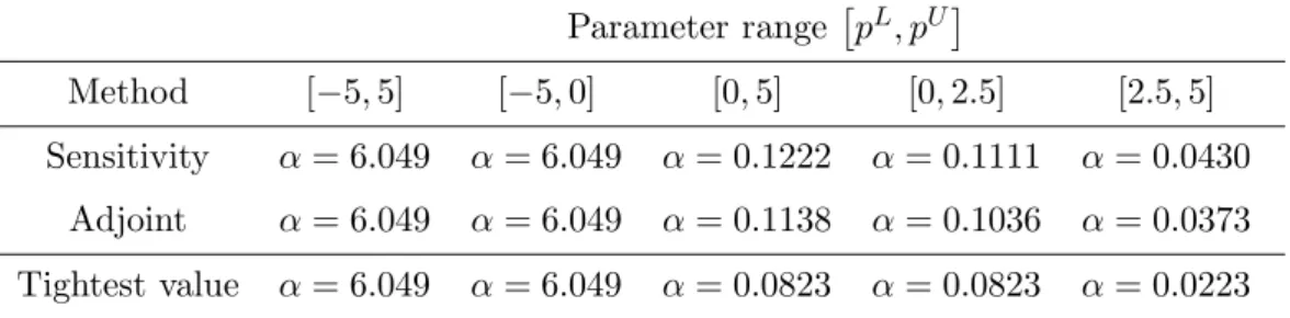
In this example, the application of the adjoint method yields tighter underestimators than the sensitivity method, but the results are close however. On the other hand, compar-isons with the optimal α coefficients indicate that both underestimating strategies provide satisfactory results. In particular, the best α-based underestimator is obtained for both strategies on the domains [−5,5] and [−5,0]. As an illustration, the functional F and its convex relaxation are pictured in Fig. 1 on different parameter domains for the adjoint underestimating procedure.
Table 1: Computation of theα coefficient for different parameter ranges pL, pU. Parameter range pL, pU Method [−5,5] [−5,0] [0,5] [0,2.5] [2.5,5] Sensitivity α= 6.049 α= 6.049 α= 0.1222 α= 0.1111 α= 0.0430 Adjoint α= 6.049 α= 6.049 α= 0.1138 α= 0.1036 α= 0.0373 Tightest value α= 6.049 α= 6.049 α= 0.0823 α= 0.0823 α= 0.0223 -40 -35 -30 -25 -20 -15 -10 -5 0 -4 -2 0 2 4 PSfrag replacements functionalF convex underestimatorF^ functional parameterp -6 -5 -4 -3 -2 -1 0 0 1 2 3 4 5 PSfrag replacements functionalF convex underestimatorF^ functional parameterp
Figure 1: FunctionalFand convex relaxation on different parameter domains for the adjoint underestimating procedure. left plot: p∈[−5,0]∪[0,5]; right plot: p∈[0,2.5]∪[2.5,5].
3.3 Spatial branch-and-bound algorithm
The optimisation problem (P) is solved to global optimality by applying the proposed un-derestimation procedure in the framework of a spatial branch-and-bound algorithm [17]. The structure of the algorithm is similar to those implemented in [11, 12]. The sequence of upper bounds on the global solution is generated by solving problem (P) to local opti-mality (see Definition 1). On the other hand, valid lower bounds on the global optimum are generated by constructing convex-underestimators for any individual function from the approach described in subsection 3.2; the lower bounding problem is thus defined as:
min p∈[pL,pU] ^ J (p) = G0 x t−1,p, . . . ,x t−ns,p,p+ ns X k=1 Z t− k t+k −1 L(k)(x,p) dt + np X i=1 α0i pUi −pi pLi −pi s.t. x˙ = f(x,p) , ∀t∈[t0, tns] x(p, t0) = h(p) 0 ≥ Gj x t−1,p , . . . ,x t−ns,p,p+ ns X k=1 Z t− k t+k −1 L(jk)(x,p) dt + np X i=1 αj i pUi −pi pLi −pi , j = 1, . . . , nc (P^)
In comparison to the convex underestimation procedure described in [11, 12, 25], it should be noted that our procedure (i) is applicable to functionals with state-dependent integral terms and, (ii) does not add any new decision variable or constraint to formulate the relaxed problem (P^). To illustrate this latter point, we consider a parameter estimation problem. For such problems, the objective is typically to minimise the weighted squared error between the observed values and those predicted by the model at given time instants. If hundreds of experimental points were considered, the application of the underestimation procedure developped in [11, 12, 25] would result in a large number of additional variables and equality constraints in the relaxed problem formulation, hence yielding a large-scale optimisation problem (and increasing the computational time). In this work however, the size of the relaxed problem remains unchanged with respect to the original problem.
Since natural interval extensions are used to compute theα values at each branch-and-bound node, the branch-and-bounding operation is improved by successive partitioning the parameter space (e.g., by applying a simple bisection rule). Guaranteedε-convergence of the algorithm is thus obtained in finite time. Note however that, apart from the quality of the lower bounding problem, the convergence of the branch-and-bound algorithm may be affected by the methods used to select the branching variable and determine appropriate variable bounds at each node of the tree.
• Two branching strategies have been investigated in this work [1]. The first one corre-sponds to the classicalleast reduced axis rule. In the second strategy, a measure of the overall influence of each variable on the tightness of the lower bounding problem is calculated, and the variable having the worst measure is selected for further bisection.
• The update of the bounds on some or any of the optimisation parameter can also be addressed at each branch-and-bound node by solving a series of additional dynamic optimisation problems (see, e.g., [11, 12]).
4
Implementation and case studies
The algorithmic procedure is implemented in an extensive Fortran90/95program. A link to the dynamic optimisation program DYNO [13] is used to perform the local optimisations; DYNOhas itself links to various local SQP solvers and integration routines (in this case,NLPQL [29] and DDASSL[8] are used). For the computation of rigorous convex underestimators for the state-dependent functionals, natural interval extensions [22] are used as inclusion func-tions due to their ease of implementation. This is done by using theINTERVAL ARITHMETIC package by Kearfott in Fortran90 [18] which performs directed outward roundings dur-ing the calculations (based on the INTLIB package). Again, the generation of lower and upper bounds on the state/costate variables and their sensitivities uses the integration routine DDASSL. Links between this program and automatic differentiation packages such as ADIFOR [6] are currently being implemented in order to generate all the necessary differentiations. Finally, it should also be noted that, to date, the program is still a proto-type implementation and, consequently, it is not optimised. Therefore, the computational times are reported only for the sake of comparison between the relaxation methods and the branching strategies.
In order to illustrate the theoretical and computational aspects of the proposed ap-proach, four example problems dealing with either parameter estimation problems from time series data or simple optimal control problems are presented. Except the first optimi-sation problem which is the continuation of the illustrative example considered throughout the paper, all other problems are taken from the book of Floudas et al. [14].
4.1 Illustrative example (continued)
In this example, the same dynamic problem used to illustrate the convex-underestimation procedure in section 3 is considered. This problem has also been addressed as an illustrative example in [25] . It is formulated as:
min p J = −x(1) 2 s.t. ˙x(t) = −x2+p , ∀t∈[0,1] x(0) = 9 −5 ≤ p ≤ 5 (P1)
It can be shown that problem P1 has two local optima (p?1,J1?) = (−5,−8.23262) and (p?2,J2?) = (5,−5.13944), i.e., one at each bound of the parameter domain. Details on the procedures applied to buildα-based convex-underestimators for the objective function have been given in section 3. Both adjoint and sensitivity based approaches are implemented here to compute the global solution. The results are given in Tab. 2.
The branching procedure is not specified in this example since the problem is mono-dimensional. For both approaches, the global optimum (p?1,J1?) is reached in 3 iterations.
Table 2: Global optimisation results for the illustrative example using different underesti-mation procedures and branching strategies.
Underestimation Branching Iterations CPU approach strategy time (s)
Sensitivity − 3 2
Adjoint − 3 7
Large differences can however be observed in terms of computational efficiency since the use of the adjoint approach leads CPU times which are three times longer; this is due to the time spent to integrate the TBPVPs. Note in particular that these results are coherent with the considerations discussed in subsection 3.1.3).
4.2 First-order irreversible series reaction
The second example concerns the estimation of the yield coefficients k1 ork2 for a two-step irreversible isothermal liquid-phase chain reaction from times series data:
A −→k1 B −→k2 C
It has been addressed in [33], as well as in [14], [12] and [25]. The parameter estimation problem involves two parametersk1,k2corresponding to the rate constants of each reaction, and two state variables x1, x2 representing the mole fractions of components A and B
respectively; it can be formulated as follow: min k1,k2 J = 10 X k=1 2 X i=1 (xi(tk)−xmesi (tk))2 s.t. ˙x1(t) = −k1x1(t) ˙ x2(t) = k1x1(t)−k2x2(t) ) ∀t∈[0,1] x1(0) = 1 x2(0) = 0 0 ≤ k1, k2 ≤ 10 (P2)
where xmesi (tk) denotes the experimental point for the ith state variable at time tk; these
values are taken from [14].
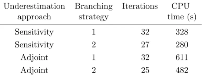
The global optimum in problem P2 is obtained for (k1, k2) = (5.0035,1.0000); the cor-responding value of the objective function at that point is J = 1.18562 10−6. The result of the global optimisation algorithm are shown in Tab. 3 for a relative tolerance of ε= 0.001. These results indicate that the adjoint approach is advantageous in terms of iterations – for the same branching strategy –,i.e., the adjoint approach yields tighter underestimators than those obtained in the sensitivity approach. On the contrary, the adjoint approach
Table 3: Global optimisation results for the first-order irreversible series reaction problem (P2) using different underestimation procedures and branching strategies.
Underestimation Branching Iterations CPU approach strategy time (s)
Sensitivity 1 32 328
Sensitivity 2 27 280
Adjoint 1 32 611
Adjoint 2 25 482
leads to much larger CPU times due to the integration of the TPBVPs (as in problemP1). Recall however that the program which is used is not optimised; we believe in particular that the efficiency of the adjoint approach could be significantly improved. On the other hand, it can be seen that the use of the branching strategy based on the underestimation quality (strategy 2) yields better results than the simple least reduced axis rule (strategy 1) – for the same type of underestimation –; the benefits can be up to 25%. Finally, it should be mentioned that the proposed approach provides the global optimum of problem P2 in fewer iterations than the approach of Papamichail and Adjiman [25] for the same relative tolerance; these results thus validate the proposed approach as a valuable tool to perform global optimisation of problems with ODEs in the constraints.
4.3 Catalytic cracking of gas oil
The third case study deals with the catalytic cracking of gas oil (A) to gasoline (Q) and other products (S). The overall reaction is given by:
A −→k1 Q
k3& .k2
S
The parameter estimation problem has been previously addressed in [33], and is also studied in [12, 25]. It can be formulated as:
min k1,k2,k3 J = 20 X k=1 2 X i=1 (xi(tk)−xmesi (tk))2 s.t. ˙x1(t) = −(k1+k3)x1(t)2 ˙ x2(t) = k1x1(t)2−k2x2(t) ) ∀t∈[0,0.95] x1(0) = 1 x2(0) = 0 0 ≤ k1, k2, k3 ≤ 20 (P3)
wherexmesi (tk) denotes the experimental point for theith state variable at time tk; again,
these values are taken from [14]. In addition,x1 anx2 are the mole fractions of components
A andQ respectively, whereas the molar fraction of componentS is unmeasured.
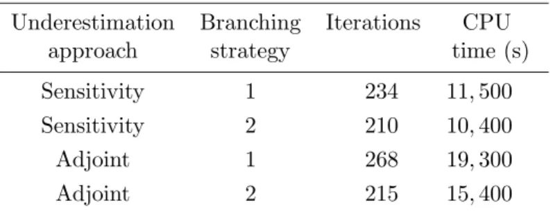
The results obtained by applying the global optimisation algorithm for different un-derestimation and branching strategies are shown in Tab. 4. In any cases, the algorithm converges to the global solution J? = 2.65567 10−3, with parameter values (k?
1, k2?, k?3) = (12.2140,7.9798,2.2217).
Table 4: Global optimisation results for the catalytic cracking problem (P3) using different underestimation procedures and branching strategies.
Underestimation Branching Iterations CPU approach strategy time (s) Sensitivity 1 234 11,500 Sensitivity 2 210 10,400 Adjoint 1 268 19,300 Adjoint 2 215 15,400
On the contrary to the results obtained in the previous examples, the sensitivity ap-proach is here preferable either in terms of iterations or with respect to the overall com-putational time. Additionally, it is also found that the branching strategy which is based on the underestimation quality (strategy 2) yields better results. One should note however, that the results reported in [25], on the same example problem, are better since convergence is obtained in less than 100 hundred iterations.
4.4 Singular optimal control problem
The last example considers a nonlinear singular optimal control problem. This problem has been studied in [19] first, and is also addressed in [27] and [11]. The problem formulation is as follow: min u(t) J = Z 1 0 x1(t)2+x2(t)2+ 0.0005 x2(t) + 16t−8−0.1x3(t) u(t)2 2 dt s.t. ˙x1(t) = x2(t) ˙ x2(t) = −x3(t)u(t) + 16t−8 ˙ x3(t) = u(t) ∀t∈[0,1] x1(0) = 0 x2(0) = −1 x3(0) = −√5 −4 ≤ u(t) ≤ 10, ∀t∈[0,1] (P4)
Note that the original problem contains an integral term which explicitly depends on time
repre-senting time,i.e., ˙x4 = 1, and then replacingtin the integral term byx4(t) (see section 2). In addition, the control variable u(t) was parameterised as a piecewise constant profile (with fixed interval lengths). These modifications reformulate problem (P4) into the form specified in Definition 1.
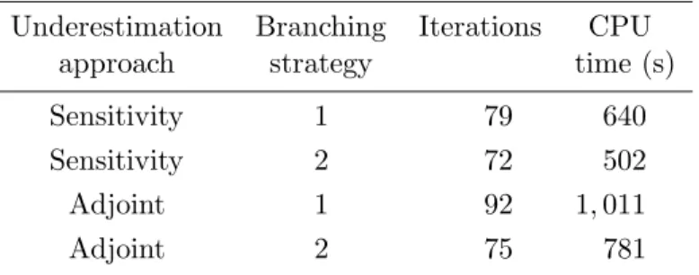
The results computed from the global optimisation algorithm with 2 control intervals are given in Tab. 5 for different underestimation procedures and branching strategies. By applying local optimisation techniques from random starting points, it can be shown that problem (P4) has at least 2 local optima: J?
1 = 0.27711 andJ2? = 0.35175, with the second one being found more frequently.
Table 5: Global optimisation results for the singular control problem (P4) using different underestimation procedures and branching strategies.
Underestimation Branching Iterations CPU approach strategy time (s)
Sensitivity 1 79 640
Sensitivity 2 72 502
Adjoint 1 92 1,011
Adjoint 2 75 781
The applications of the global optimisation approach yields the global optimum J?
1 in any case, with parameters (u?1, u?2) = (5.5748,−4.0000). As in the previous example, the use of the sensitivity based approach is preferable here since it improves the convergence to the global solution; the second branching option also achieves faster convergence results than the standard least reduced axis rule.
5
Conclusions and perspectives
In this paper, a deterministic global optimisation algorithm has been presented to solve problems with ordinary differential equations in the constraints. The algorithm is built on a spatial branch-and-bound framework. The novelty is in the procedure applied to derive convex relaxations of the original nonconvex dynamic optimisation problems. Convex underestimators are derived for each individual nonconvex twice continuously differentiable state-dependent functionals by adding a convex quadratic term of which weight coefficient
α can be computed rigorously based on either a sensitivity or an adjoint based approach. Both uses the concept of differential inequalities to compute bounds on the state trajectories of ODE systems.
A prototype implementation of the algorithm has been realised in Fortran90 and the approach is tested on several simple parameter estimation and optimal control problems taken from the literature. The results suggest that both sensitivity and adjoint based approaches provide accurate convex underestimators for nonconvex functionals. It was found that the use of either one of the approaches may be advantageous depending on
the optimisation problem. It is worth noticing that the results are close in any case. In addition, the branching strategy has a large influence on the convergence of the algorithm. The use of branching strategy quantifying the influence of each variable on the tightness of the underestimator, rather than the standard least reduced axis rule was found to improve the convergence in all case studies. Finally, these theoretical and practical considerations validate the proposed method as an alternative approach to the optimisation of problems with ODEs in the constraints.
Current investigations are focussed on the application of this deterministic global op-timisation algorithm to larger dynamic opop-timisation problems, and in particular problems with many decision variables such as those resulting from the application of control param-eterisation techniques. For these problems, we believe that the application of the adjoint based approach might be preferable since its complexity increases linearly with the num-ber of decision variables. In addition, the need to derive tight convex underestimators will be even more crucial for large-scale optimisation problems in order to compute the global solution in reasonable computational times.
References
[1] Adjiman C. S., Dallwig S., Floudas C. A. and Neumaier A. (1998a), “A global optimiza-tion method, αBB, for general twice differentiable constrained NLPs – I. Theoretical advances”,Computers and Chemical Engineering, 22(9):1137-1158.
[2] Adjiman C. S., Dallwig S. and Floudas C. A. (1998b), “A global optimization method,
αBB, for general twice differentiable constrained NLPs – II. Implementation and com-putational results”,Computers and Chemical Engineering,22(9):1159-1179.
[3] Androulakis I., Maranas C. D. and Floudas C. A. (1995), “αBB: A global optimization method for general constrained nonconvex problems”,Journal of Global Optimization,
7:337-363.
[4] Banga J. R. and Seider W. D. (1996), “Global optimization of chemical processes using stochastic algorithms”, In: “State of the Art in Global Optimization”, C. A. Floudas and P. M. Pardalos Editors, Series in nonconvex optimization and its applications, pp. 563-583, Dordrecht, Kluwert Academic Publishers.
[5] Biegler L. T. (1984), “Solution of dynamic optimization problems by successive quadratic programming and orthogonal collocation”, Computers and Chemical En-gineering, 8(3/4):243-248.
[6] Bischof C., Carle A., Corliss G., Griewank A., Hovland P. (1992), ”ADIFOR- Generating Derivative Codes from Fortran Programs” Scientific Programming, 1:1-29.
[7] Boender C. G. and Romeijn H. E. (1995), “Stochastic methods”, In: “Handbook of Global Optimization”, R. Horst and P. M. Pardalos Editors, Series in nonconvex opti-mization and its applications, pp. 829-869, Dordrecht, Kluwert Academic Publishers. [8] Brenan K. E., Campbell S. E. and Petzold L. R. (1989), “Numerical solution of initial
[9] Bryson A. E. and Ho Y. C. (1975), “Applied Optimal Control”, Hemisphere Publishing Corporation.
[10] Chachuat B. and Latifi M. A. (2002), “GDO: afortran90program for global optimisa-tion of problems with ordinary differential equaoptimisa-tions”,Technical report, LSGC-CNRS (Nancy, France), in preparation.
[11] Esposito W. R. and Floudas C. A. (2000a), “Deterministic global optimization in nonlinear optimal control problems”,Journal of Global Optimization, 17:96-126. [12] Esposito W. R. and Floudas C. A. (2000b), “Global optimization for the parameter
estimation of differential-algebraic systems”, Industrial & Engineering Chemistry Re-search, 39(5):1291-1310.
[13] Fikar M. and Latifi M. A. (2002), “User’s guide for fortran dynamic optimisation codeDYNO”,Technical report, LSGC-CNRS (Nancy, France) & STU Bratislava (Slovak Republic)”.
[14] Floudas C. A., Pardalos P. M., Adjiman C. S., Esposito W. R.,G¨um¨us Z. H., Harding S. T., Klepeis J. L., Meyer C. A. and Schweiger C. A. (1999), “Handbook of test problems in local and global optimization”, Series in nonconvex optimization and its applications, Dordrecht, Kluwert Academic Publishers.
[15] Frank P. M. (1978), “Introduction to System Sensitivity Theory”, Academic Press, New York.
[16] Harrison G. W. (1979), “Compartmental models with uncertain flow rates”, Mathe-matical Biosciences, 43:131-139.
[17] Horst R. and Tuy H. (1996), “Global Optimization. Deterministic Approaches” (3rd edition), Springer-Verlag, Berlin.
[18] Kearfott R. B. (1996), “INTERVAL ARITHMETIC: A Fortran90 module for an interval data type”,ACM Transaction on Mathematical Software, 22(4):385-392.
[19] Luus R. (1990), “Optimal control by dynamic programming using systematic reduction in grid size”,International Journal of Control, 51(5):995-1013.
[20] Luus R. (1992), “Mutiplicity of solutions in the optimization of a bifunctional catalyst blend in a tubular reactor”,Canadian Journal of Chemical Engineering, 70:780-785. [21] Maranas C. D. and Floudas C. A. (1994), “Global minimum potential energy
confor-mations of small molecules”,Journal of Global Optimization, 4:135-170. [22] Moore R. E. (1966), “Interval Analysis”, Prentice-Hall, Engelwood Cliffs, NJ.
[23] Moore R. E. (1979), “Methods and Applications of Interval Analysis”, SIAM, Philadel-phia, PA.
[24] Neuman C. and Sen A. (1973), “A suboptimal control algorithm for constraint problems using cubic splines”, Automatica, 9:601-613.
[25] Papamichail I. and Adjiman C. S. (2002), “A rigorous global optimization algorithm for problems with ordinary differential equations”, Journal of Global Optimization,
24:1-33.
[26] Pontriagin L. (1962), “The Mathematical Theory of Optimal Processes”, Interscience Publishers, New York.
[27] Rosen O. and Luus R.(1997), “Global optimization approach to nonlinear optimal control”,Journal of Optimization Theory & Applications, 73:547-562.
[28] Ruban A. I. (1997), “Sensitivity coefficients for discontinuous dynamic systems”, Jounal of Computer and System Sciences International, 36(4):536-542.
[29] Schittkowski K. (1985), “NLPQL: a Fortran Subroutine Solving Constrained Nonlinear Programming Problems”,Annals of Operations Research”, 5(6):485-500.
[30] Singer A. B. and Barton P. I. (2003), “Global solution of linear dynamic embedded op-timization problems – Part I: Theory”,Journal of Optimization Theory & Applications,
Submitted for publication.
[31] Smith E. M. and Pantelides C. C. (1995), “Global optimisation of general process models”, In: “Global optimization in engineering design”, I.E. Grossmann Editor, Series in nonconvex optimization and its applications, Chapter 12, pp. 355-386, Dordrecht, Kluwert Academic Publishers.
[32] Teo K., Goh G. and Wong K. (1991), “A Unified Computational Approach to Optimal Control Problems”, Pitman Monographs and Surveys in Pure and Applied Mathemat-ics, John Wiley & Sons, Inc., New York, 1991.
[33] Tjoa I. B. and Biegler L. T. (1991), “Simulatneous solution and optimization strate-gies for parameter estimation of differential-algebraic equation systems”,Industrial & Engineering Chemistry Research, 30:376-385.
[34] Tsang T. H., Himmelblau D. M. and Edgar T. F. (1975), “Optimal control via collo-cation and nonlinear programming”, International Jounal of Control, 21(5):763-768. [35] Vassiliadis V. S., Canto E. B. and Banga J. R. (1999), “Second-order sensitivity of
general dynamic systems with application to optimal control problems”,Chemical En-gineering Science, 54(17):3851-3860.
[36] Vassiliadis V. S., Sargent R. W. and Pantelides C. C. (1994a), “Solution of a class of multistage dynamic optimisation problems – 1. Problems without path constraints”, Industrial & Engineering Chemistry Research, 33(9):2111-2122.
[37] Vassiliadis V. S., Sargent R. W. and Pantelides C. C. (1994b), “Solution of a class of multistage dynamic optimisation problems – 2. Problems with path constraints”, Industrial & Engineering Chemistry Research, 33(9):2123-2133.