Data-driven model development in
environmental geography
Methodological advancements and scientific
applications
kumulative
Dissertation
zur Erlangung des Doktorgrades
der Naturwissenschaften
(Dr. rer. nat.)
dem Fachbereich Geographie
der Philipps-Universität Marburg
vorgelegt von
Hanna Meyer
aus Oberhausen
Erstgutachter: Prof. Dr. Thomas Nauß Zweitgutachter: Prof. Dr. Bernhard Seeger Drittgutachter: Prof. Dr. Andreas Huth Tag der mündlichen Prüfung: 08.02.2018
Preface
At the end of a challenging but yet inspiring and special time, I would like to thank those people who supported and accompanied me on this journey. First of all, I would like to sincerely thank Thomas Nauß for providing the opportunity to write this thesis, his great support throughout the entire process and eventually for always allowing more than just a few (spatial and scientific) detours. Further, I would like to express my deep gratitude to Chris Reudenbach for his support in so many ways, that I could always count on and that I appreciate a lot.
I am also very grateful to my colleagues in the working group of environmental informatics. The time would not have been as special without them as they provided a great working (and beyond) environment that is certainly unique. As the first steps are always the hardest, I am especially thankful to Meike Kühnlein for introducing me to the field of rainfall modelling. Further, thanks go to Alice Ziegler for proofreading the envelope of this thesis and her valuable comments.
However, I would not have been there without the early support of Jörg Bendix and Boris Thies who were responsible that I could acquire a taste in science during my studies. In this context, I would further like to thank Lukas Lehnert for many years of fruitful dicussions, sharing knowledge, ideas and field experiences.
This thesis was embedded in the BMBF funded IDESSA project and would not have been possible without this financial support. It further relyed on data from several institutions that I would like to acknowledge at the end of each respective chapter of my thesis. The papers of this thesis were developed in collaboration with several people. I would like to thank all co-authors for their contributions and I am grateful to Caley Gasch, Tom Hengl, Karoline Messenzehl and Marwan Katurji for giving me the chance to contribute to their projects. Special thanks go to Marwan Katurji and Peyman Zawar-Reza for welcoming me in New Zealand several times and for introducing me to the Antarctic research. I am also thankful to the IDESSA team for scientific discussions and help during field work.
Last but not least, the thesis could not have been developed without the gen-eral support of my family and friends. I am very thankful to my neighbours Stefan, Anneke and Lotta for distraction after work and to Nic, for patiently proofreading my papers and much more importantly for being an awesome part-ner for mountain adventures in New Zealand and beyond. Finally, very special thanks go to my sister Nele for never-ending scientific discussions and especially for being an invaluable mate in life.
Hanna Meyer Marburg, July 2017
Abstract
One key task in environmental geography is obtaining information of geo-graphic features in space or in space and time. For this purpose, modelling strategies are needed that allow a delineation of spatio-temporal information based on limited field data. In this context, the nonlinearity and complexity of environmental systems require modelling strategies that allow handling arbitrary relationships and large sets of potential predictor variables. These requirements provoke a paradigm-shift from a parametric towards a non-parametric and data-driven model development which is strengthened by an increasing availability of geographic data. In that respect, machine learning algorithms have been proven to be an important tool to learn patterns in nonlinear and complex systems. While the large number of machine learning applications in scientific journals as well as recent software developments nowadays feign a simplicity of these methods, their application is not a trivial task. This holds especially true for ge-ographic data as they have certain characteristics, especially spatial dependency, that make them stand out against the mass of "ordinary" data. However, this is widely ignored in geographic machine learning applications.
This thesis assesses the potential and the sensitivity of machine learning in environmental geography. In this context, a number of machine learning appli-cations in a broad spectrum of environmental geography have been published, providing a collection of comprehensive knowledge about machine learning in environmental geography. The individual contributions are incorporated in the major hypothesis that, only if characteristics of geospatial data are considered, data-driven modelling strategies lead to a reliable gain of information and to ro-bust spatio-temporal model results. Beside this superior methodological focus, each application aims at providing new insights in its respective field of research. In this thesis, a number of relevant environmental monitoring products have been developed. The results emphasize that a high expertise of the machine learn-ing methods as well as of the scientific field is crucial to advance the environmental geography. The thesis is the first to raise awareness of spatial or spatio-temporal over-fitting in geographic machine learning applications and the significant con-sequences to the outcome. To approach this problem, a new method for model development is provided that is adapted for geographic data and allows for im-proved model results. The thesis is finally an appeal to think beyond the "stan-dard machine learning way" as it proves that applying stan"stan-dard machine learning concepts on geographic data results in considerable over-fitting and misinterpre-tation of the results. Only when characteristics of geographic data are considered, machine learning provides a powerful tool to provide scientifically valuable results in environmental geography.
Zusammenfassung
Die Erfassung räumlich kontinuierlicher Daten und raum-zeitlicher Dynamiken ist ein Forschungsschwerpunkt der Umweltgeographie. Zu diesem Ziel sind Mo-dellierungsmethoden erforderlich, die es ermöglichen, aus limitierten Felddaten raum-zeitliche Aussagen abzuleiten. Die Komplexität von Umweltsystemen er-fordert dabei die Verwendung von Modellierungsstrategien, die es erlauben, be-liebige Zusammenhänge zwischen einer Vielzahl potentieller Prädiktoren zu berück-sichtigen. Diese Anforderung verlangt nach einem Paradigmenwechsel von der parametrischen hin zu einer nicht-parametrischen, datengetriebenen Modellent-wicklung, was zusätzlich durch die zunehmende Verfügbarkeit von Geodaten ver-stärkt wird. In diesem Zusammenhang haben sich maschinelle Lernverfahren als ein wichtiges Werkzeug erwiesen, um Muster in nicht-linearen und kom-plexen Systemen zu erfassen. Durch die wachsende Popularität maschineller Lernverfahren in wissenschaftlichen Zeitschriften und die Entwicklung komforta-bler Softwarepakete wird zunehmend der Fehleindruck einer einfachen Anwend-barkeit erzeugt. Dem gegenüber steht jedoch eine Komplexität, die im Detail nur durch eine umfassende Methodenkompetenz kontrolliert werden kann. Diese Problematik gilt insbesondere für Geodaten, die besondere Merkmale wie vor allem räumliche Abhängigkeit aufweisen, womit sie sich von "gewöhnlichen" Daten abheben, was jedoch in maschinellen Lernanwendungen bisher weitestgehend ig-noriert wird.
Die vorliegende Arbeit beschäftigt sich mit dem Potenzial und der Sensitivität des maschinellen Lernens in der Umweltgeographie. In diesem Zusammenhang wurde eine Reihe von maschinellen Lernanwendungen in einem breiten Spek-trum der Umweltgeographie veröffentlicht. Die einzelnen Beiträge stehen unter der übergeordneten Hypothese, dass datengetriebene Modellierungsstrategien nur dann zu einem Informationsgewinn und zu robusten raum-zeitlichen Ergebnissen führen, wenn die Merkmale von geographischen Daten berücksichtigt werden. Neben diesem übergeordneten methodischen Fokus zielt jede Anwendung darauf ab, durch adäquat angewandte Methoden neue fachliche Erkenntnisse in ihrem jeweiligen Forschungsgebiet zu liefern.
Im Rahmen der Arbeit wurde eine Vielzahl relevanter Umweltmonitoring-Produkte entwickelt. Die Ergebnisse verdeutlichen, dass sowohl hohe fachwissen-schaftliche als auch methodische Kenntnisse unverzichtbar sind, um den Bereich der datengetriebenen Umweltgeographie voranzutreiben. Die Arbeit demons-triert erstmals die Relevanz räumlicher Überfittung in geographischen Lernan-wendungen und legt ihre Auswirkungen auf die Modellergebnisse dar. Um diesem Problem entgegenzuwirken, wird eine neue, an Geodaten angepasste Methode zur Modellentwicklung entwickelt, wodurch deutlich verbesserte Ergebnisse erzielt
werden können. Diese Arbeit ist abschließend als Appell zu verstehen, über die Standardanwendungen der maschinellen Lernverfahren hinauszudenken, da sie beweist, dass die Anwendung von Standardverfahren auf Geodaten zu starker Überfittung und Fehlinterpretation der Ergebnisse führt. Erst wenn Eigenschaften von geographischen Daten berücksichtigt werden, bietet das maschinelle Lernen ein leistungsstarkes Werkzeug, um wissenschaftlich verlässliche Ergebnisse für die Umweltgeographie zu liefern.
VII
Contents
Preface I
Abstract III
Zusammenfassung V
List of Figures XIII
List of Tables XVII
List of Acronyms XIX
1 Introduction 2
1.1 Modeling tasks in environmental geography . . . 2
1.2 Predictive modelling strategies . . . 4
1.2.1 Classic modelling strategies . . . 5
1.2.1.1 Spatial Interpolations . . . 5
1.2.1.2 Statistical parametric models . . . 6
1.2.2 The paradigm shift towards data-driven model development 7 1.3 Machine learning fundamentals and terminology . . . 8
1.4 Machine learning in environmental geography - State of the art . . 9
1.4.1 Biogeography . . . 10
1.4.2 Climatology . . . 10
1.4.3 Soil science and hydrology . . . 11
1.4.4 Geomorphology . . . 11
1.5 Formulation of the scientific problem, aims and hypotheses . . . . 12
1.5.1 Characteristics of geographic data . . . 12
1.5.2 Aims and hypotheses . . . 13
1.5.3 Concept and structure of this thesis . . . 14
2 Comparison of ML algorithms for rainfall retrievals 18 2.1 Introduction . . . 19
2.2 Data and methodology . . . 20
2.2.1 Datasets . . . 21
2.2.1.1 Satellite data . . . 21
2.2.1.2 RADOLAN RW data . . . 22
2.2.2 Preprocessing of SEVIRI and Radar data . . . 22
2.2.3 Predictor variables . . . 23
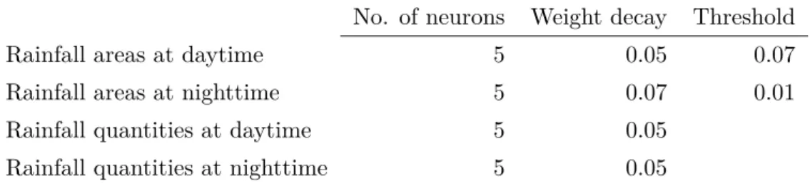
2.2.5 Model tuning . . . 25
2.2.5.1 Random forests tuning . . . 25
2.2.5.2 NNET and AVNNET tuning . . . 26
2.2.5.3 SVM tuning . . . 26
2.2.5.4 Threshold tuning for rainfall area classification models . . . 26
2.2.6 Model prediction and validation . . . 27
2.2.6.1 Validation of rainfall area classification models . . 27
2.2.6.2 Validation of rainfall rates regression models . . . 28
2.3 Results . . . 29
2.3.1 Comparison of predicted rainfall areas . . . 29
2.3.2 Comparison of predicted rainfall rates . . . 30
2.4 Discussion . . . 30
2.4.1 Prediction of rainfall areas . . . 30
2.4.2 Prediction of rainfall rates . . . 32
2.4.3 Technical considerations . . . 35
2.5 Summary and conclusions . . . 36
3 Spectral and textural predictors for rainfall retrievals 40 3.1 Introduction . . . 41
3.2 Methods . . . 42
3.2.1 Satellite and ground truth data . . . 43
3.2.2 Compilation of training and test data sets . . . 44
3.2.3 Neural network training . . . 45
3.2.3.1 Recursive feature selection . . . 45
3.2.3.2 Fine tuning and model training . . . 46
3.3 Results . . . 46
3.4 Discussion and Conclusion . . . 47
4 Satellite-based mapping of rainfall over southern Africa 52 4.1 Introduction . . . 53
4.2 Methods . . . 54
4.2.1 Study area . . . 55
4.2.2 Data and Preprocessing . . . 56
4.2.2.1 Station data . . . 56
4.2.2.2 Satellite data . . . 56
4.2.2.3 Cloud mask . . . 57
4.2.3 Model strategies for rainfall estimation . . . 57
4.2.3.1 General model framework . . . 57
IX
4.2.3.3 Tuning and model training . . . 59
4.2.3.4 Spatial estimations of rainfall . . . 60
4.2.4 Validation . . . 60 4.2.5 Comparison to GPM . . . 61 4.3 Results . . . 62 4.3.1 Model performance . . . 62 4.3.2 Comparison to GPM . . . 63 4.4 Discussion . . . 65 4.5 Conclusions . . . 69
5 Mapping daily air temperature for Antarctica 72 5.1 Introduction . . . 73
5.2 Methods . . . 74
5.2.1 Data and Preprocessing . . . 74
5.2.1.1 LST . . . 74
5.2.1.2 Station Records . . . 75
5.2.1.3 Auxiliary Data . . . 75
5.2.1.4 Compilation of Model Training and Testing Data 76 5.2.2 Modelling . . . 76
5.2.2.1 Algorithms . . . 76
5.2.2.2 Cross-Validation Strategies and Feature Selection to Minimize Overfitting . . . 77
5.2.2.3 Final Model Training, Evaluation and Prediction . 78 5.3 Results . . . 79
5.3.1 Selected Features . . . 79
5.3.2 Model Comparison and Evaluation . . . 80
5.4 Discussion . . . 86
5.5 Conclusions . . . 88
6 From spectral measurements to maps of pasture degradation 92 6.1 Introduction . . . 93
6.2 Data and methods . . . 94
6.2.1 Study area . . . 94
6.2.2 Field work . . . 95
6.2.2.1 Spectral measurements . . . 96
6.2.2.2 Proxies for pasture degradation . . . 97
6.2.3 Satellite data . . . 97
6.2.4 Methodology to remotely derive pasture degradation pa-rameters . . . 97
6.2.4.2 Estimation of pasture degradation parameters
us-ing Random Forests . . . 99
6.2.4.3 Regionalization . . . 100
6.3 Results . . . 101
6.3.1 Feature selection and predictive importance of NBIs . . . . 101
6.3.2 Accuracies of estimations based on hyper- and multispec-tral data . . . 101
6.3.3 Application to satellite data . . . 103
6.4 Discussion . . . 105
6.5 Conclusions . . . 109
7 Classifying woody vegetation in Google Earth images 112 7.1 Introduction . . . 113
7.2 Methods . . . 114
7.2.1 Study area . . . 115
7.2.2 Data and variables . . . 115
7.2.3 Random Forests classification . . . 117
7.2.4 Validation . . . 117
7.2.5 Prediction on new Google Earth images . . . 118
7.3 Results and Discussion . . . 119
7.3.1 Model performance and variable importance . . . 119
7.3.2 Database of training sites . . . 120
7.4 Conclusions . . . 123
8 Spatio-temporal interpolation of soil properties in 3D+T 126 8.1 Introduction . . . 127
8.2 Materials and methods . . . 129
8.2.1 The Cook Agronomy Farm data set . . . 129
8.2.2 Conceptual foundation for 3D+T modeling . . . 131
8.2.3 3D+T random forests model . . . 132
8.2.4 3D+T kriging model . . . 134
8.2.5 Cross-validation . . . 138
8.2.6 Software implementation . . . 139
8.3 Results . . . 140
8.3.1 3D+T random forests model . . . 140
8.3.2 3D+T kriging model . . . 140
8.3.3 Model accuracy . . . 142
8.4 Discussion . . . 144
8.4.1 Model performance . . . 144
XI
8.4.3 Final conclusions and future directions . . . 149
9 Soil respiration based on mid-infrared spectroscopy 154 9.1 Introduction . . . 155
9.2 Material and Methods . . . 156
9.2.1 Study area . . . 156
9.2.2 Soil sampling . . . 157
9.2.3 Determination of physicochemical soil properties . . . 158
9.2.4 Soil respiration measurements and determination of Q10 . . 158
9.2.5 Mid infrared spectroscopy (MIRS) . . . 160
9.2.6 Relation between MIRS spectra and soil respiration param-eters . . . 160
9.2.7 Partial least square regression (PLSR) . . . 160
9.2.8 Random Forest modeling . . . 161
9.3 Results and Discussions . . . 162
9.3.1 MIRS-PLSR based prediction of soil respiration at stan-dardized temperature and moisture . . . 162
9.3.2 MIRS-PLSR based prediction of Q10 values . . . 163
9.3.3 Simultaneous prediction of soil respiration across various levels of soil moisture and temperature by Random Forest modeling . . . 166
9.4 Conclusion . . . 170
10 Regional-scale controls of rockfalls 172 10.1 Introduction . . . 174
10.2 Characteristics of the study area . . . 177
10.3 Modelling approach . . . 178
10.3.1 Data selection and pre-processing . . . 178
10.3.1.1 Response variable . . . 178
10.3.1.2 Predictor variables . . . 179
10.3.2 Validation methodology . . . 182
10.3.3 Principal component analysis and logistic regression mod-elling . . . 183
10.3.4 Random forest model . . . 185
10.4 Results . . . 186
10.4.1 Spatial characteristics of rockfall source areas (rockfall den-sity statistics) . . . 186
10.4.2 Principal components and geomorphic meaning . . . 187
10.4.3 PCLR model and importance of PCs . . . 188
10.4.4 Random forest model and variable importance . . . 191
10.5 Discussion . . . 193
10.5.1 Evaluation of the methodological approach . . . 193
10.5.2 Regional-scale controls on rockfall activity . . . 195
10.5.2.1 The predisposing effect of rock mechanical char-acteristics . . . 195
10.5.2.2 Paraglacial adjustment processes as system inher-ent controls . . . 197
10.5.2.3 Topo-climatic forcing on permafrost rockwalls . . 200
10.6 Perspectives . . . 202
10.7 Conclusion . . . 203
11 Improving the performance of spatio-temporal models 206 11.1 Introduction . . . 207
11.2 Case studies and description of the datasets . . . 209
11.2.1 Case Study I: modelling air temperature in Antarctica . . . 209
11.2.2 Case Study II: modelling volumetric water content of the "Cookfarm", USA . . . 210
11.3 Methods . . . 210
11.3.1 Random Forest algorithm . . . 210
11.3.2 Validation strategies . . . 212
11.3.3 Feature selection . . . 212
11.4 Results and Discussions . . . 214
11.4.1 Target-oriented validation . . . 214
11.4.2 Detecting over-fitting . . . 215
11.4.3 Reducing over-fitting and improving model performances . 215 11.5 Conclusions . . . 221
12 Conclusions 224 12.1 Significance of the developed products . . . 224
12.2 Opportunities of machine learning in geography . . . 226
12.3 Challenges of machine learning in geography . . . 227
12.4 Accounting for space-time dependencies . . . 228
12.5 Practical consequences . . . 229 12.6 Outlook . . . 231 12.7 Concluding remarks . . . 231 References 233 Curriculum Vitae 274 Erklärung 279
XIII
List of Figures
1.1 A very simple interpolation of rainfall . . . 6
1.2 A very brief description of the process of machine learning . . . 9
1.3 Structure of this work . . . 15
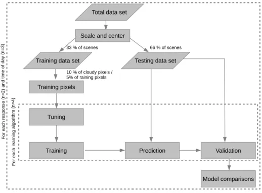
2.1 Flow chart of the main methodology applied in this study . . . 21
2.2 Example of threshold tuning . . . 25
2.3 Comparison of the rainfall area prediction performances of the four ML algorithms . . . 31
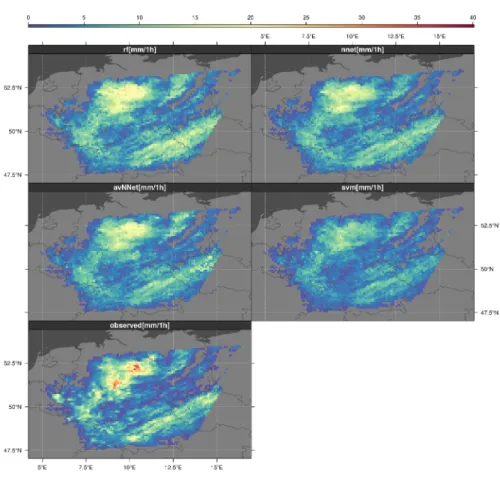
2.4 IR image of the MSG SEVIRI scene from 2010/05/06 14:50 UTC . 32 2.5 Visualization of the rainfall area predictions of the four ML algo-rithms for the exemplary scene . . . 33
2.6 Comparison of the rainfall rate prediction performances of the four ML algorithms . . . 34
2.7 Visualization of the 24-hour aggregated rainfall rate predictions of the four ML algorithms for the exemplary day . . . 35
3.1 Overview of the methods to compare models that use spectral and textural variables with models that use spectral variables only . . . 43
3.2 Dependence of the number of variables on the performance . . . . 47
3.3 Boxplots showing the performance of the full models as well as spectral-only models . . . 48
4.1 Flow chart of the methodology applied in this study . . . 54
4.2 Map of the average annual precipitation sums in the study area as estimated by WordClim . . . 55
4.3 Validation of estimated rainfall areas for 2013 on an hourly basis . 62 4.4 Comparison of POD for different hourly measured rainfall quanti-ties as well as FAR for different predicted rainfall quantiquanti-ties . . . . 63
4.5 Validation of estimated rainfall quantities for 2013 on an hourly basis . . . 63
4.6 Validation of estimated rainfall quantities for 2013 at (a) hourly resolution and on the different aggregation (b) daily, (c) weekly, (d) monthly . . . 64
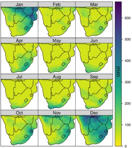
4.7 Monthly precipitation sums in mm of the year 2013 as estimated by this study . . . 65
4.8 Comparison of the performance of the MSG based retrieval and GPM IMERG for rainfall area delineation between March and Au-gust 2014 . . . 66
4.9 Comparison of the performance of the MSG based retrieval and GPM IMERG for hourly rainfall quantities between March and August 2014 . . . 67
4.10 Sample satellite scene from 2014/04/24 10:00 UTC as well as the rainfall estimates for this scene, observed rainfall and GPM IMERG estimates . . . 68
5.1 Map of weather stations used for model training and evaluation . . 76 5.2 Relative variable importance revealed by Cubist . . . 80
5.3 Agreement between measuredTairand predictedTair using Cubist
as modeling tool . . . 81
5.4 Correlation between measured and predictedTair based on LOSOCV 82
5.5 Distribution of measured Tair compared to predictedTair . . . 82
5.6 Measured and predicted time series of three example weather stations 83
5.7 Monthly RMSE ofTair predictions for stations on ice and ice-free
areas . . . 84
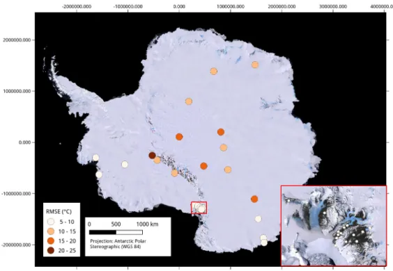
5.8 Spatial distribution of RMSE of predictedTair for the 32 weather
stations . . . 84
5.9 Performance of theTair product on different aggregation levels . . 85
5.10 Monthly aggregates ofTair as predicted by the GBM model . . . . 85
6.1 Map of the study area including vegetation types as well as the position of the sampling locations . . . 95 6.2 Schema of the processing flow . . . 99
6.3 R2 values of linear regressions between NBI and vegetation cover . 102
6.4 R2 values of linear regressions between NBI and AGB . . . 103
6.5 Example of the spatial predictions at the loation "Qumahe" . . . . 104 6.6 Validation of the vegetation cover models . . . 105 6.7 Validation of the AGB models . . . 105 6.8 Distribution of vegetation cover values at the different locations
where satellite data was available . . . 106 6.9 Distribution of biomass values at the different locations where
satellite data was available . . . 106 7.1 Overview of the processing flow . . . 115 7.2 Map of the study area including the location of training images as
well as images used for prediction . . . 116 7.3 Variable importance of 15 highest ranked predictor variables in the
Random Forests model . . . 120 7.4 Reliability of 500 Google Earth images . . . 122 7.5 Three example RGB images, the predicted probabilities for woody
vegetation and the corresponding classification results . . . 122 8.1 Cook Agronomy Farm overview map with soil profile sampling
points and instrumented locations . . . 132 8.2 Sensor values from five depths at one station at Cook Agronomy
Farm . . . 133 8.3 Distribution of observations for water content, temperature, and
electrical conductivity across soil depth . . . 134 8.4 Importance plots (covariates sorted by importance) . . . 141
XV
8.5 Spatio-temporal predictions of soil water content at Cook Agron-omy Farm for the growing season in 2012 using the random forests
(RF) model . . . 142
8.6 Spatio-temporal sample variogram, metric variogram, and isolated 3D spatial and temporal components . . . 144
8.7 Spatio-temporal predictions of soil water content at Cook Agron-omy Farm for the growing season in 2012 using the kriging model . 145 8.8 Hexbin plots for observed and predicted values showing goodness of fit . . . 146
8.9 Types of soil variables in terms of temporal stability or change . . 151
9.1 Comparison between measured and predicted soil respiration (SR) rates at 25°C and 45% of water holding capacity based on leave-one-out cross validation . . . 164
9.2 Correlation between absorption at each wavenumber and SOC, SR25,45, Q10, and SOC-degradability for the general dataset and the individual subsets . . . 165
9.3 Baseline-corrected MIRS spectra of three grassland soils . . . 165
9.4 Comparison between measured and predicted Q10 values based on leave-one-out cross validation . . . 167
9.5 Comparison between measured and predicted soil respiration rates based on leave-one-sampling-point-out cross-validation . . . 168
9.6 Comparison between measured and predicted soil respiration rates based on leave-one-sampling-point-out cross-validation for each land use type separately . . . 169
9.7 Scaled variable importance as revealed by the Random Forest al-gorithm . . . 169
10.1 Process-scale of potential rockfall controls . . . 176
10.2 Study area . . . 178
10.3 Selection of predictor variables . . . 182
10.4 Modelling approach of the multiple logistic regression . . . 184
10.5 Rockfall densities (RD in %) of predictor variables . . . 187
10.6 Variable importance quantified by means of the random forest mode191 10.7 Receiver Operating Characteristic . . . 192
10.8 Typical examples for active talus slope deposition . . . 197
10.9 Possible models for the timing of paraglacial rockfall activity in the Turtmann Valley . . . 199
11.1 Schematic overview of validation strategies considered in this study 213 11.2 Differences in the Leave-Location-Out cross-validation performance of a) the air temperature estimations and b) the volumetric water content estimations using different feature selection strategies . . . 219
11.3 Relative scaled importance of the predictor variables within the Random Forest models for the case study of (a) Tair Antarctica and (b) VW Cookfarm . . . 220
11.4 Differences in the Leave-Location-Out and Leave-Location-and-Time-Out cross-validation performance using no feature selection, a recursive feature elimination and the newly proposed forward feature selection . . . 220
XVII
List of Tables
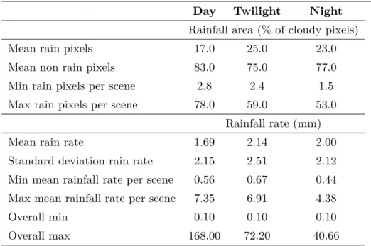
2.1 Summary of rainfall areas and rainfall rates of the three input
datasets . . . 23
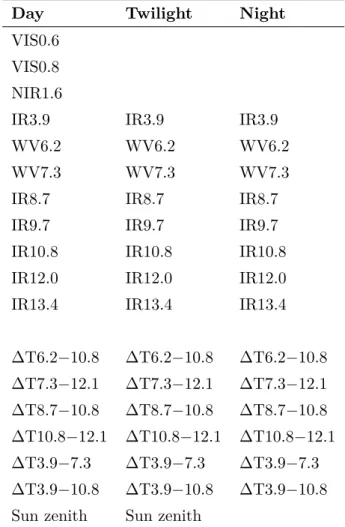
2.2 Overview of the predictor variables used to model rainfall areas and rainfall rates . . . 24
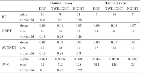
2.3 Optimal tuning parameters . . . 27
2.4 Confusion matrix as baseline for the calculation of the verification scores . . . 28
2.5 Calculation of the confusion matrix-based verification scores . . . . 28
2.6 Processing time in minutes for model tuning and training as well as just model training with the optimal tuning parameters . . . 36
4.1 Optimal hyperparameters for the individual models . . . 60
4.2 Confusion matrix as baseline for the calculation of the verification scores . . . 61
4.3 Categorical metrics for validation of rainfall area estimates . . . 61
5.1 Tested values for the hyperparameters of the different prediction models and the optimal parameters revealed during parameter tuning 79 6.1 Overview of the 18 locations which were sampled during field work in 2011 and 2012 . . . 96
6.2 Summary statistics of the vegetation cover and AGB samples . . . 97
6.3 Overview of the spectral bands of the three satellite sensors Quick-Bird, RapidEye and WorldView-2 . . . 98
6.4 Summary of the satellite images which were available for this study 98 6.5 Cross validated results of the feature selection with RF training for the different models calculated in this study . . . 102
7.1 Confusion matrix . . . 118
7.2 Cross tabulation based validation metrics . . . 119
7.3 Contingency table of the test data set . . . 120
7.4 Performance of the Random Forests model . . . 120
7.5 Excerpt of the training site database for the three example images shown in Fig. 7.5. . . 121
8.1 Cook Agronomy Farm data set spatio-temporal covariates . . . 135
8.2 Parameters of the seasonality functions for water content (VW), soil temperature (C) and electrical conductivity (EC) . . . 143
8.3 Variogram parameters for each variable . . . 143
8.4 Global cross-validation statistics . . . 147
9.1 Environmental soil classes (ESC) and sample set . . . 158
9.2 Prediction accuracy forSR25,45, Q10 values, and C-degradability (i.e.,SR25,45/SOC, SOC normalized soil respiration) based on the different submodels . . . 166
10.2 Diagnostics statistics of multicollinearity between independent pre-dictors . . . 185 10.3 Varimax-rotated principal components of original standardised
pre-dictor variables . . . 189 10.4 Test for goodness-of-fit . . . 190 10.5 Coefficient statistics . . . 190 10.6 Contingency table for the principal component logistic regression
model and the random forest model . . . 192 11.1 Predictor variables used within the two case studies . . . 211 11.2 Regression statistics between observed and predicted values based
XIX
List of acronyms
AGB Aboveground Biomass
AIC Akaike Information Criterion
AUC Area Under the Curve
AVNNET Averaged Neural Network
BLD Bulk density of soil
Bt Occurrence of Bt horizon
cdayt Transformed cumulative day
CLM Community Land Model
CSI Critical Success Index
CV Cross-Validation
DEM Digital Elevation Model
DTM Digital Terrain Model
EC Electrical Conductivity
ESC Environmental Soil Classes
ETS Equitable Threat Score
FAR False Alarm Ratio
FFS Forward Feature Selection
GLCM Grey Level Co-occurance Matrix
GBM Generalized Boosted Regression Models
GPM Global Precipitation Measurement
HKD Hansen-Kuipers Discriminant
HSS Heidke Skill Score
IMERG Integrated Multi-satellite Retrievals for GPM
IR Infrared
LLO Leave-Location-Out
LLTO Leave-Location-and-Time-Out
LOSOCV Leave-One-Station-Out Cross-Validation
LR Logistic Regression
LST Land Surface Temperature
LTO Leave-Time-Out
MAE Mean Absolute Error
ME Mean Error
MIRS Mid-Infrared Spectroscopy
ML Machine Learning
MODIS Moderate-resolution Imaging Spectroradiometer
MSG Meteosat Second Generation
mtry Number of variables randomly sampled at
each split
NBI Narrow-Band Indices
NDRE Normalized Difference Red-Edge Index
NDVI Normalized Difference Vegetation Index
NIR Near Infrared
NNET Neural Network
ntree Number of trees
PC Principal Components
PCLR Principal Component Logistic Regression
PHI Soil pH
PLSR Partial Least Square Regression
POD Probability Of Detection
POFD Probability Of False Detection
Q10 Increase of soil respiration by a 10◦C
XXI
QB Quickbird
QTP Qinghai-Tibet-Plateau
R2
Coefficient of determination
RAMP Radarsat Antarctic Mapping Project
RE Rapid Eye
RF Random Forest
RFE Recursive Feature Elimination
RMSE Root Mean Square Error
ROC Receiver Operating Characteristic
sd Standard deviation
SEVIRI Spinning Enhanced Visible and Infrared Imager
SOC Soil Organic Carbon
SR Soil Respiration
SRREF Soil Respiration at a reference temperature
SVM Support Vector Machines
Tair Air Temperature
TREF Reference Temperature
TRMM Tropical Rainfall Measuring Mission
UTC Coordinated Universal Time
VIF Variation Inflation Factors
VIS Visible
VVI Visible Vegetation Index
VW Volumetric Water Content
WHC Water Holding Capacity
Chapter 1
1
Introduction
One of the key tasks in environmental geography is obtaining information of geographic features in space or in space and time. Considering current trends
towards big data, increasing volume, velocity, and variety of geographic data
(van Zyl, 2014) lead to new opportunities for environmental monitoring that are accompanied with a paradigm shift towards data-driven data analysis. In this context, machine learning algorithms learn patterns in nonlinear and complex systems. That makes them an important tool in environmental geography that is highly associated with nonlinearity and complex underlying interactions. Whilst the number of machine learning applications in environmental geography rapidly increases, the characteristics of geographic data (especially spatial dependencies) remain widely unconsidered in geographic machine learning applications.
The following introduction will give an overview on the modelling tasks in environmental geography and the necessary paradigm shift towards data-driven model development. Based on limitations and challenges of recent machine learn-ing applications, the aim and hypotheses of this thesis are developed followed by a description of the general outline of this thesis.
1.1 Modeling tasks in environmental geography
To understand the potential for data-driven modelling in environmental geog-raphy, it is worth clarifying the major tasks in geography that require modelling approaches.
• Mapping of geographic features
A frequent task in geography is obtaining spatially explicit information of environmental features based on limited field observations. Thus, small scale data records are transferred into space to obtain maps of the feature of interest. Mapping of geographic features is a common task in all fields of environmental geography. In biogeography, mapping of land cover (Gómez
et al., 2016) or biodiversity (Miller, 1994) are common applications. In soil science and geomorphology, mapping of soil characteristics (McBrat-ney et al., 2003; Breviket al., 2016) and geomorphological features (Smith
et al., 2011) are routine. The aims of spatial mapping are diverse and serve several purposes like policy making and planning of e.g. conservation areas according to biodiversity characteristics (Ferrier, 2002). Spatial mapping in geography is further used as a tool for risk assessment, e.g. of
1.1 Modeling tasks in environmental geography 3
flooding (Porter and Demeritt, 2012). In addition, spatially explicit data serve as essential baseline products that subsequent scientific studies can build upon.
• Spatio-temporal monitoring of geographic features
Whilst some geographic features can be considered as being temporally comparably static (e.g. soil types), other features are highly dynamic not only in space but also in time (e.g. soil moisture). Therefore, spatio-temporal monitoring extends the approach of spatio-temporally static mapping of geographic features by considering temporal dynamics. The aim of a spatio-temporal monitoring is to obtain dynamics of a certain feature in space and time. Potential areas for application in environmental geography are the monitoring of dynamic vegetation characteristics as e.g.
phenol-ogy (Zhang et al., 2003). In climatology, most variables of interest are
even more dynamic than vegetation characteristics, as for example air
tem-perature (Hengl et al., 2011) or rainfall (Kidd and Huffman, 2011). The
variability of climate has an impact on other spheres that react in a highly dynamic way. Soil temperature or soil moisture for example react on the dynamic climatic impacts and its spatio-temporal monitoring is an
impor-tant field in soil science (Gasch et al., 2015). Spatio-temporal monitoring
allows analysing dynamics and trends and form valuable tools for planning,
policy making (Ceccatoet al., 2014) and as baseline products for scientific
studies. • Forecasting
Spatio-temporal dynamics are not only studied from past and present times, but predictions are also made into the future. Forecasting is especially rele-vant in the field of climatology with regard to short term weather forecasts and long-term trends. Climate change predictions are the most prominent example in this context (IPCC, 2014). Forecasting also plays a role in other disciplines, for example concerning projections of land use and land cover
change (Veldkamp and Lambin, 2001; Thies et al., 2014). By building
sce-narios of future behaviour, forecasting is an essential tool for policy making and to develop strategies for adaptation (IPCC, 2014).
• Enhancing knowledge about system behaviour
Another aim in environmental geography that requires modelling is the understanding of system behaviour. It is a question of how individual components influence a system and how a system reacts to changing condi-tions (Bossel, 1994). Examples from the field of biogeography and climatol-ogy could be gaining knowledge about vegetation-atmosphere interactions
(Krinner et al., 2005) while in geomorphology the delineation of factors
As it is apparent from the list of modelling tasks, there are two general targets pursued: Mapping, monitoring as well as forecasting of geographic features aim at creating accurate maps, time series or scenarios, while the second target is associated with system understanding and the identification of driving forces that lead to those spatial or spatio-temporal patterns. These two general targets are approached with two different categories of models: predictive models and explanatory models (Shmueli, 2010).
Predictive models (Kuhn and Johnson, 2013a) in environmental geography are mainly statistical. Such models are built upon the statistical relationship be-tween field data of the target and spatially available predictor data (e.g. remote sensing data). As a very simple example, we could assume the task of mapping air temperature using the assumption of decreasing air temperature with increas-ing elevation. The statistical model is established from ground observations of air temperature (i.e. via climate stations) and corresponding information about elevation. The developed model can then be applied on the entire set of the spatially available data (i.e. digital elevation model) to obtain spatially explicit temperature estimates. While predictive models aim at accurate estimations of a feature in space and time (i.e. monitoring of air temperature), the explanatory models aim at an accurate understanding of processes and interactions (i.e. how is elevation related to air temperature?). Explanatory models can be statistical where potential influencing factors are tested for their relationship to the tar-get, or conceptual or physical (Gray and Gray, 2017) where the model aims at representing a simplified representation of a system.
In this thesis, I will focus on predictive models, however, with consideration of explanatory components. Main emphasis will be on modelling strategies for spatial mapping and spatio-temporal monitoring. Though most of the content is applicable to the modelling task of forecasting as well, forecasting is not explicitly considered in this thesis.
1.2 Predictive modelling strategies
In view to the task of spatial mapping and spatio-temporal monitoring, it is a question of how the spatial or spatio-temporal dynamics of a parameter can be obtained. The initial situation is that we usually have point data (e.g. from climate stations) or data from small scale surveys (e.g. vegetation plot records) available that give us the geographic feature of interest for certain spatial locations and at certain points in time. However, initially we do not know anything about the feature’s behaviour beyond the sample locations and beyond the date of the survey.
1.2 Predictive modelling strategies 5
In the following sections, the pathway from point or small scale data to spa-tially explicit and temporally continuous data will be outlined. First, the "classic" approaches will be discussed followed by the delineation of the need towards data-driven model development.
1.2.1 Classic modelling strategies
1.2.1.1 Spatial Interpolations
The most obvious approach to obtain spatially explicit data might evolve from
Tobler’s first law of geography that implies "everything is related to everything
else, but near things are more related than distant things"" (Tobler, 1970). This law established the basis for the concept of spatial interpolations. The principle of spatial interpolations is that the characteristics of a feature are spatially cor-related and therefore, point data can be transferred into space according to the distance.
Let’s consider the task of spatio-temporal monitoring of hourly rainfall to illus-trate the idea and problems associated with the concept of spatial interpolations. As an example, we have a number of climate stations distributed over southern Africa, that measure precipitation on an hourly resolution. However, we want to know rainfall for the entire area of southern Africa. According to the idea of interpolation, recorded rainfall values at a certain point in time (Fig. 1.1A) are interpolated by considering the distance to the climate stations (e.g. using a simple kriging interpolation, Fig. 1.1B). However, two problems are associated with this approach. The first problem becomes obvious by visual interpretation of the resulting map (Fig. 1.1B). Though the interpolation might have produced reliable results in the areas where the density of climate stations was high, the results become highly unreliable in areas with a low density of stations. Ob-viously, as rainfall is a highly dynamic parameter, a spatial interpolation that simply bases on the distance to the weather stations does not produce satisfying results. Admittedly, the example shown here is very simple. Though it could be extended by using a more complex interpolation approach, e.g. including further explanatory predictors as e.g. elevation (Goovaerts, 2000) or by using more
com-plex algorithms (Ly et al., 2011), there is a second problem that is associated
with this concept. Using spatial interpolations, monitoring is restricted to the date where field records are available as the concept relies on the field data. Thus, if no field data are available, no spatial mapping can be performed. Considering the example of rainfall monitoring, this problem might be of low relevance since modern data loggers quasi-continuously produce data. However, other studies rely on temporally restricted data when field surveys are of high temporal and economic costs (e.g. vegetation surveys).
Due to the continuous dependence on field data as well as the lack of a suitabil-ity for dynamic variables, spatial interpolations do not provide a comprehensive and satisfying solution for the task of spatio-temporal monitoring when dealing with highly dynamic features and spatially or temporally limited ground truth data. Therefore, other approaches are required.
m m No Rainfall No Data m m No Rainfall No Data A B
Figure 1.1: A very simple interpolation of rainfall in southern Africa from 2014/04/24 10:00. A shows the measured rainfall from several climate stations (Meyer
et al., 2017a). B shows the results from a simple kriging approach.
1.2.1.2 Statistical parametric models
Another well-established way for spatial mapping or spatio-temporal monitor-ing uses spatially available proxies or predictors for the feature of interest. With regard to remote sensing, there is much information available from space, that can be related to geographical features or processes by regression or classification anal-ysis. Examples include the increase of biomass with increasing satellite-retrieved
NDVI (Gizachew et al., 2016), the relationship between satellite-based surface
temperature and air temperature (Vogtet al., 1997), or the increasing
probabil-ity for rainfall with decreasing cloud temperatures that as well are provided by
satellites (Vicenteet al., 1998).
Once a statistical model is built between satellite data and the response vari-able, it can be applied to the full extent of the satellite scene, or even to a time series, allowing spatial mapping or spatio-temporal monitoring of the response
(e.g. Gizachewet al., 2016; Shiet al., 2016; Loprestiet al., 2015, to mention just
a few). By using this strategy, we got rid of the dependency on continuously available field data because once the model is built, no further ground truth data are required.
A model using just one predictor variable might, however, only in rare cases provide a good estimate of the response variable. Usually more than a single predictor is required to explain a feature’s characteristic. Though common para-metric models can also be of a more complex form and include more than one
1.2 Predictive modelling strategies 7
2012), the parametric approaches have a significant limitation: they are based on an a priori assumption of the data distribution (Breiman, 2001b) as well as of
the form of the relationship between predictors and response (Jameset al., 2013).
This form is often assumed to be linear but can also be exponential or even more complex. While it is still possible to assess the appropriate relationship between predictor and response when only one or very few predictors are used, it becomes nearly impossible to assess the individual relationships when a large number of predictors is considered. A large number of predictors is further problematic in view to multicollinearity (Graham, 2003). Since most geographic data are correlated (e.g. spectral reflectance in different wavelengths), and this behaviour cannot be included in most parametric models, a considerable reduction in the number of predictors is often necessary from a technical perspective. Most sys-tems, however, can only be described by a large number of interacting predictor variables and behave in a nonlinear manner. This problem raises the need for more flexible models that can handle large numbers of predictors, different types of variables and arbitrary relationships.
1.2.2 The paradigm shift towards data-driven model development
As more and more (spatial) data become available the requirement for more flexible models force a paradigm shift towards true data-driven model develop-ment (Miller and Goodchild, 2015). Data-driven model developdevelop-ment, or what
Breiman (2001b) refers to asalgorithmic modelling in contrast todata modelling,
is a designation associated with big data and aims at finding relationships in
the data without an a priori assumption about the system (Breiman, 2001b;
Lary et al., 2016). In this context, machine learning algorithms are applied as a predictive modelling tool to learn arbitrary relationships in the data and to make predictions according to the learned function. The advantage compared to parametric approaches is that machine learning algorithms learn relationships between predictors and responses by themselves. This allows a greater flexibility and the utilization of many, correlated, or even potentially uninformative pre-dictor variables. In this context it is of note that the greater flexibility is at the expense of interpretability. Machine learning algorithms are referred to as a
black box because the exact learned relationship between predictors and response
is difficult to interpret (Laryet al., 2016). However, machine learning algorithms
are advantageous when prediction is in the foreground rather than an exact un-derstanding of underlying relationships. Therefore, they have high potential for mapping or monitoring of geographic features.
In general, we can distinguish between two categories of learning: supervised
learning and unsupervised learning (James et al., 2013). Supervised learning
measurements). The aim of supervised applications is to learn how the predictors can best describe the response. In contrast, unsupervised learning is based on predictor variables solely, thus there is no response variable and the data are
considered to beunlabelled. The aim of unsupervised learning is then to structure
the predictor variables in a way that a subsequent labelling of the data is possible. According to the major modelling tasks outlined in section 1.1, this thesis focus on supervised learning tasks. The fundamentals of supervised machine learning will be explained in the following.
1.3 Machine learning fundamentals and terminology
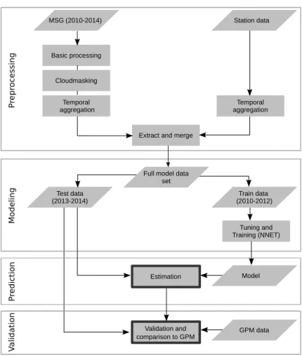
Machine learning is a collective term for a variety of data-driven algorithms that aim at learning the relationship between predictor and response variables and make predictions based on the developed model. A usual modelling task (Fig. 1.2) starts with the acquisition of the target variable which is also referred
to asresponse variable,dependent variable orground truth. Usually this is data
taken from field surveys or data loggers. Predictor variables (also referred to as
independent variables) are then required to estimate theresponse variable. Predictor and response variables form the initial dataset which is then split intotrainingandtesting data, thus into data that is used totrainthe model, and
data that is used to validate or test the model. Based on the training data, a
machine learning algorithm then learns the relationship between predictors and
response which is designated asmodel training. Most machine learning algorithms
have so calledhyperparameters ortuning parametersthat control the model
com-plexity which cannot be directly estimated from the data (Kuhn and Johnson,
2013a). Therefore, atuning of these parameters must be included in the process
of model training.
Both, model tuning and model training, must always be evaluated in view to
independent data, thus the effect of the hyperparameters as well as the perfor-mance of the final model must always be evaluated with held back data. If this is not considered, the resulting model has a high risk of over-fitting because highly complex models are able to fit to noise in the training data. This, however, is not applicable for the general relationship between predictors and response (James
et al., 2013). In this context, cross-validation has been evaluated as a robust tool to tune the complexity of models to avoid over-fitting (Kuhn and Johnson,
2013a; James et al., 2013). For cross-validation, the data are split into several
folds(resamples). For each iteration, a model is trained with a respective set of hyperparameters using all data except for one fold and the performance of the model to predict on the held back fold is then assessed. In this way, the optimal set of hyperparameters can be retrieved and an objective performance metric of
1.4 Machine learning in environmental geography - State of the art 9
the final model can be given.
Once the model is trained, it can be applied on an entire set of predictors
to make predictions in space, or on a new set of predictors to make predictions
in space and time. It is of note, that the term prediction in this context is not
synonymous to the term forecast. Though predictions might be made for future
conditions, the term more generally means to estimate the response variable for unknown data, thus for locations where no ground truth data were available or for unknown points in time (within a defined model domain).
Finally, it is of note that supervised machine learning can aim at two different
tasks: regression orclassification. While the response of classification models is
categorical (e.g. land cover classes), the response of regression models is contin-uous ornumeric.
Algorithm
Learns relations Model
Predictors Response Predictors New set Prediction/ Estimation Data set Validation
Figure 1.2: A very brief description of the process of machine learning. The grey col-ored shapes represent data, orange the modelling procedure and yellow the outcome.
1.4 Machine learning in environmental geography - State of the art
Machine learning algorithms are well-established in environmental sciences
(Lary et al., 2016; Kanevski et al., 2009; Hsieh, 2009) and find application in all
fields of environmental geography. In this context, machine learning is widely used in conjunction with remote sensing (see review in Paola and Schowengerdt, 1995; Lary et al., 2016; Camps-Valls, 2009; Mountrakiset al., 2011) as it provides an excellent source for spatial and spatio-temporal predictor variables for a variety of environmental research tasks. The following section gives a brief - by no means exhaustive - overview where machine learning is used in different fields of environmental geography.
1.4.1 Biogeography
One of the typical applications of machine learning in the field of biogeog-raphy is the mapping of land use/cover based on optical satellite information
(Gislasonet al., 2006; Rodriguez-Galiano et al., 2012). In this context, machine
learning algorithms, as for example neural networks or support vector machines, have shown to be superior compared to traditional methods such as the
maxi-mum likelihood classifier (Huanget al., 2002; Otukei and Blaschke, 2010; Waske
et al., 2009). Using machine learning and multispectral data, land cover could be classified into broad vegetation types and the use of hyperspectral data allowed
further classification down to a species level (Baldecket al., 2015; Lawrenceet al.,
2006). Multispectral, as well as hyperspectral data, in conjunction with machine
learning are further used to map vegetation cover (Lehnert et al., 2015b),
bio-physical characteristics (Verrelst et al., 2012), biomass (Ali et al., 2015) or tree
diversity (Vaglio Laurin et al., 2014). Ground truth data for these studies were
usually provided by field surveys where vegetation characteristics were sampled on a plot scale.
Whilst spectral satellite data can be considered to be directly related to vegeta-tion patterns, machine learning was used in modelling tasks, where more indirect predictor variables were applied. Baltensperger and Huettmann (2015) mod-elled the diversity of mammals in Alaska using derived remote sensing products that included land cover, climatological information as well as terrain properties. Habitat suitability was also modelled with machine learning on derived remote
sensing products, for example to obtain potential habitats forPinus sylvestrison
the Iberian Peninsula (Garzónet al., 2006).
1.4.2 Climatology
Machine learning has a long-term history in the field of spatial atmospheric
sci-ence. Cloud type classifications (Tianet al., 1999; Giannakos and Feidas, 2013),
cloud characteristics (Junget al., 1998) as well as rainfall (Hsuet al., 1997; Hong
et al., 2004; Behrangi et al., 2009a; Kühnleinet al., 2014b) were modelled using
machine learning. With a few exceptions (Kühnlein et al., 2014a,b), artificial
neural networks are the prevailing algorithms in the field of cloud and rainfall modelling. This is in contrast to other fields of environmental geography, where a high variability of algorithms is applied. The idea behind cloud and rainfall
retrievals is that the spectral information (e.g. optical, Kühnleinet al., 2014b) is
related to cloud properties which are further related to rainfall probabilities. As well as monitoring climatic patterns, machine learning was applied as an alter-native statistical downscaling approach for general circulation models (Tripathi
1.4 Machine learning in environmental geography - State of the art 11
As climate provides boundary conditions for other systems (Bonan, 2008), climate monitoring products are of high relevance for subsequent studies, e.g. as important predictors for biodiversity mapping (Baltensperger and Huettmann, 2015).
1.4.3 Soil science and hydrology
The application of machine learning in soil science and hydrology is rather recent but of increasing interest to the scientific community. A large field of
ap-plication is mapping of soil taxonomic units (see review in Heunget al., 2016) but
also mapping of soil properties like soil moisture (Ahmad et al., 2010; Ali et al.,
2015), soil organic carbon (Ließet al., 2016; Hendersonet al., 2005), or nitrogen
and phosphorus content (Henderson et al., 2005). As ground truths, point
obser-vations from soil samples or soil profiles are being used and the response variable is usually predicted from topographic information, spectral satellite data and/or
climate indices (Heung et al., 2016).
Another application of machine learning that also has the aim to provide high resolution soil moisture datasets is the downscaling of low resolution
satellite-based soil moisture products with higher resolution predictors (Srivastavaet al.,
2013; Im et al., 2016).
In regard to hydrology, machine learning finds frequent application in
stream-flow modelling and forecasting (Rasouli et al., 2012; Asefa et al., 2006;
Short-ridgeet al., 2016). However, these applications are usually not spatially explicit
but focus on temporal patterns. Space as well as time, however, recently found consideration in machine-learning based run-off modelling (Gudmundsson and Seneviratne, 2015). Further hydrological applications of machine learning are compiled in Govindaraju and Rao (2000).
1.4.4 Geomorphology
The most common application of machine learning in geomorphology is the
mapping of landslide susceptibility (Micheletti et al., 2014; Catani et al., 2013;
Goetz et al., 2015; Brenning, 2005) which reaches into the field of risk
assess-ment. Machine learning was also applied to map landforms, for example types
of glaciated landscapes (Brown et al., 1998). Machine learning applications for
1.5 Formulation of the scientific problem, aims and hypotheses
As outlined in section 1.4, machine learning is used in all fields of environmen-tal geography and the number of applications is considerably increasing. Machine learning, however, is not a very recent discovery in environmental geography. In contrast, machine learning to obtain spatio-temporal datasets from limited ground truth data was already applied in the 1990s, however, at this time, due to the high complexity of application, it was only used by experts in this field. Major developments in software packages in recent years, allow greater access to machine learning for virtually everyone. Well-known GIS software (ArcGIS, SAGA, QGIS, GRASS, IDRISI, etc) provides easily accessible machine learning functionality for environmental mapping. Especially R, as a frequently used software in natural science, has a variety of machine learning algorithms implemented (Hothorn,
2017). The caret package for R (ClassificationAndREgressionTraining, Kuhn,
2016a) allows access to most of the implemented algorithms via a handy and uni-fied syntax and further provides a variety of functions for data processing, model tuning and evaluation, parallel computing as well as model visualization.
While the large number of machine learning applications in scientific journals, as well as the today user-friendly software, feign a simplicity of machine learning, the complexity of the methods has not changed with time. Underestimating the technical complexity increases the risk of incorrect utilization of algorithms and can lead to false interpretations and conclusions. This is especially problematic in the field of geography since machine learning algorithms were not originally developed for spatial and spatio-temporal data analysis and the common work-books that serve as guidelines on how machine learning is used (e.g. Kuhn and
Johnson, 2013a; James et al., 2013) do not refer to geographic data. Therefore,
machine learning algorithms in geography are usually applied in the same way as in statistical medicine, economics, and other non-spatial fields. However, geo-graphic data have certain characteristics (see section 1.5.1) that make them stand out against the mass of "ordinary" data and this should have serious consequences for the utilization of machine learning in geography.
1.5.1 Characteristics of geographic data
The most obvious and important characteristic of geographic data is surely
its localisation in space (geospatial data). Geospatial data refer to a location
on ground and provide data of a variable at the corresponding location. Vector point data might be the most intuitive example for geospatial data and the most frequent type of ground truth data for prediction models. Point data can be linked to a point on earth by its coordinates and a reference system and include certain information about a geographic feature at this point (e.g. via data loggers
1.5 Formulation of the scientific problem, aims and hypotheses 13
on climate stations). In contrast, the majority of earth observation data and the main source of predictor variables being used in predictive models are provided
by remote sensing (Lary et al., 2016) and typically represented as raster data.
Raster data provide discrete or continuous information of geographic features in a spatially explicit way. Especially such spatially explicit data illustrate one of the key characteristics of geospatial data: they are within a certain degree dependent in space causing spatial patterns to mostly appear as either patches or
gradients (Legendre, 1993). This dependence of a variable in space causesspatial
autocorrelation. Spatial autocorrelation means that samples are more/less similar than what might be expected from a random distribution (Legendre, 1993). The geographic feature at location "x" depends in a certain way on the feature on neighbouring locations and/or on the environmental characteristics not only of the location "x" itself but also of the neighbourhood. Thus, observations (i.e. spatial pixels or points) are not independent of each other.
Autocorrelation of geospatial data does not only happen in space but also in
time (Shen et al., 2016). Especially when time series of geographic features are
to be analysed (e.g. air temperature, soil moisture, vegetation greenness), the
observations at one point often feature a temporal autocorrelation resulting in
dependency in space and time (spatio-temporal autocorrelation).
Though spatial and spatio-temporal autocorrelation is probably the key char-acteristic, geographic data have further characteristics that might be important in view to machine learning applications. The irregularity of many geographic features lead to unbalanced data, e.g. considering the ratio between raining and
non raining clouds (Kühnlein et al., 2014b) which is highly unbalanced as the
averaged proportion of non raining clouds is considerably higher compared to raining clouds. Further, geographic datasets feature a large variability in size. Often large amounts of potential predictor variables (e.g. via remote sensing) contrast with only a few samples of response variables (e.g. vegetation surveys). These characteristics (especially the spatial and/or temporal dependency) make geographic data special when compared to the standard data used in other scientific fields. This raises the question if, and how, these characteristics need to be incorporated in machine learning applications.
1.5.2 Aims and hypotheses
This thesis aims at assessing the potential and sensitivity of machine learning for environmental geography. In this context, as the characteristics of geographic data are being widely ignored in the large amount of recent machine learning applications, the superior aim of this thesis is to advance the field of machine learning in environmental geography by addressing these characteristics. The
thesis is developed in view to the hypothesis that, only if the characteristics of geographic data are considered, data-driven modelling strategies lead to a gain of information and to robust spatio-temporal model results.
Therefore, based on a variety of environmental monitoring applications, the thesis aims at developing adequate modelling strategies with respect to charac-teristics of geographic data, to provide reliable spatio-temporal data from lim-ited field observations that support knowledge about different ecosystem compo-nents. The series of applications provides the basis to discuss the influence of geographic data and consequent modelling strategies in the general context of machine learning-based spatio-temporal monitoring of the environment.
1.5.3 Concept and structure of this thesis
During this thesis, a number of contributions in a broad spectrum of environ-mental geography have been published so that this thesis presents a collection of comprehensive knowledge about machine learning in environmental geogra-phy. The individual contributions are incorporated in the major hypothesis that, if characteristics of geospatial data are not considered, data-driven modelling strategies lead neither to a gain of information nor to robust spatio-temporal model results. Each chapter further provides new insights or monitoring prod-ucts in its respective field of research.
Within this thesis the individual contributions are structured according to their field of research (Fig. 1.3). Chapters 2, 3 and 4 thematically focus on rainfall retrieval based on optical satellite data. Chapter 5 further covers this climatological context and aims at developing a spatio-temporal satellite-based monitoring product of air temperature for Antarctica. From the field of bio-geography, chapter 6 evaluates different hyperspectral and multispectral indices to map vegetation cover and biomass on the Qinghai-Tibet-Plateau. Chapter 7 presents a method to automatically create Google Earth based training data for a larger scale monitoring of bush encroachment in South Africa. From the field of soil science, chapter 8 addresses modelling soil properties in space, time and depth on a farm scale and chapter 9 aims at developing a model to obtain soil respiration estimates from mid-infrared data. In a geomorphological context, chapter 10 aims at identifying factors that lead to rockfall in the Turtmann Val-ley in the Swiss Alps. The final publication in this thesis (chapter 11) wraps up the findings from the individual case studies by addressing the problem of spatio-temporal over-fitting due to the characteristics of geospatial data.
The key findings of this thesis could only be a result of a development process and are consequently maturing over the individual publications. Therefore, the final chapter of this thesis (chapter 12) summarizes the major methodological
1.5 Formulation of the scientific problem, aims and hypotheses 15
developments from this study and discusses them in the broader methodological context. This chapter will further highlight the scientific outcome of the individ-ual chapters and give recommendations for the utilization of machine learning in environmental geography.
Chapter 2
Meyer, H., Kühnlein, M., Appelhans, T., Nauss, T. (2016):Comparison of four machine learning algorithms for their applicability in satellite-based optical rainfall retrievals.Atmospheric Research, 169, Part B, 424–433.
Chapter 3
Meyer, H., Kühnlein, M., Reudenbach, C., Nauss, T. (2017):Reveiling the potential of spectral and textural predictor variables in a neural network-based rainfall retrieval technique.Remote Sensing Letters, 8, 647-656.
Chapter 4
Meyer, H., Drönner, J., Nauss, T. (2017):
Satellite-based high-resolution mapping of rainfall over southern Africa. Atmospheric Measurement techniques, 10, 2009-2019.
Chapter 5
Meyer, H., Katurji, M., Appelhans, T., Müller, M.U., Nauss, T., Roudier, P., Zawar-Reza, P. (2016): Mapping daily air temperature for Antarctica based on MODIS LST.Remote sensing, 8, 732.
Chapter 6
Meyer, H., Lehnert, L.W., Wang, Y., Reudenbach, C., Nauss, T., Bendix, J. (2017): From local spectral measurements to maps of vegetation cover and biomass on the Qinghai-Tibet-Plateau: Do we need hyperspectral information?
International Journal of Applied Earth Observation and Geoinformation, 55, 21-31.
Chapter 7
Ludwig A., Meyer H., Nauss T. (2016):
Automatic classification of Google Earth images for a larger scale monitoring of bush encroachment in South Africa.International Journal of Applied Earth Observation and Geoinformation, 50, 89-94.
Chapter 10
Messenzehl, K., Meyer, H., Otto, J., Hoffmann, T., Dikau, R. (2017):
Regional-scale controls on the spatial activity of rockfalls (Turtmann valley, Swiss Alps) – A multivariate modelling approach.
Geomorphology, 287, 29-45.
Chapter 8
Gasch, C., Hengl, T., Gräler, B., Meyer, H., Magney, T., Brown, D.J. (2015):
Spatio-temporal interpolation of soil moisture, temperature, and electrical conductivity in 3D+T: the Cook Farm data set. Spatial Statistics, 14 (A), 70-90.
Chapter 9
Meyer, N., Meyer, H., Welp, G., Amelung, W. (submitted): Soil respiration and its temperature sensitivity: rapid acquisition using mid-infrared spectroscopy.
Geoderma.
N. Meyer
Chapter 11
Meyer, H., Reudenbach, C., Hengl, T., Katurji, M., Nauss, T. (submitted):
Improving performance of spatio-temporal machine learning models using forward feature selection and target-oriented validation.
Environmental Modelling & Software
Chapter 12
Conclusions
Biogeography
Climatology Soil Science Geomorphology
H.Meyer H.Meyer N.Meyer N.Meyer
Chapter 2
Comparison of four machine learning
algorithms for their applicability in
satellite-based optical rainfall retrievals
Hanna Meyer (1), Meike Kühnlein (1), Tim Appelhans (1), Thomas Nauß (1)
(1) Environmental Informatics, Faculty of Geography, Philipps-University Marburg, Deutschhausstr. 10, 35037 Marburg, Germany
Published in
Atmospheric Research 2016, 169 Part B, 424–433
Received 10 December 2014Revised 19 September 2015 Accepted 22 September 2015 Available online 8 October 2015

![A modular family of phosphine phosphoramidite ligands and their hydroformylation catalysts : steric tuning impacts upon the coordination geometry of trigonal bipyramidal complexes of type [Rh(H)(CO)2(P^P*)]](data:image/gif;base64,R0lGODlhAQABAIAAAP///wAAACH5BAEAAAAALAAAAAABAAEAAAICRAEAOw==)