2018
Some Bayesian methods for univariate density
estimation
Kathleen Rey
Iowa State UniversityFollow this and additional works at:
https://lib.dr.iastate.edu/etd
Part of the
Statistics and Probability Commons
This Dissertation is brought to you for free and open access by the Iowa State University Capstones, Theses and Dissertations at Iowa State University Digital Repository. It has been accepted for inclusion in Graduate Theses and Dissertations by an authorized administrator of Iowa State University Digital Repository. For more information, please [email protected].
Recommended Citation
Rey, Kathleen, "Some Bayesian methods for univariate density estimation" (2018).Graduate Theses and Dissertations. 16866. https://lib.dr.iastate.edu/etd/16866
A dissertation submitted to the graduate faculty in partial fulfillment of the requirements for the degree of
DOCTOR OF PHILOSOPHY
Major: Statistics
Program of Study Committee: Stephen Vardeman, Co-major Professor
Daniel Nordman, Co-major Professor Petrutza Caragea
Heike Hofmann Max Morris
The student author, whose presentation of the scholarship herein was approved by the program of study committee, is solely responsible for the content of this dissertation. The Graduate College will ensure this dissertation is globally accessible and will not permit alterations after a degree is
conferred.
Iowa State University Ames, Iowa
2018
DEDICATION
I would like to dedicate this thesis to my parents, Mary and Tim, for their never-ending support and prayers throughout my graduate school career.
Page
LIST OF TABLES . . . viii
LIST OF FIGURES . . . ix ACKNOWLEDGEMENTS . . . xxiii ABSTRACT . . . xxiv CHAPTER 1. DUOS . . . 1 1.1 Introduction . . . 1 1.1.1 Literature Review . . . 3
1.1.1.1 Non-Bayesian Density Estimation . . . 3
1.1.1.2 Bayesian Density Estimation . . . 6
1.2 Methods . . . 13 1.2.1 Introduction . . . 14 1.2.2 Data Model . . . 16 1.2.3 Priors . . . 18 1.2.4 Posterior Distributions . . . 20 1.2.5 Gibbs Sampling . . . 28 1.2.5.1 Rejection Sampling . . . 30 1.2.6 Gibbs Algorithm . . . 34 1.3 Results . . . 36 1.3.1 Convergence . . . 37 1.3.2 Evaluation . . . 48 1.3.3 PDF and CDF . . . 54 1.3.4 Statistics . . . 61
1.4 Extension . . . 65 1.5 Discussion . . . 70 CHAPTER 2. GOLD . . . 72 2.1 Introduction . . . 72 2.2 Literature Review . . . 73 2.3 Methods . . . 77 2.3.1 Data Model . . . 77 2.3.2 Priors . . . 82 2.3.3 Posterior . . . 83 2.3.4 Metropolis-Hastings Algorithm . . . 85 2.4 Results . . . 86 2.4.1 Convergence . . . 88 2.4.2 Evaluation . . . 94 2.4.3 PDF and CDF . . . 99 2.4.4 Statistics . . . 107 2.5 Discussion . . . 112 CHAPTER 3. R PACKAGE . . . 116 3.1 Introduction . . . 116 3.2 DUOS . . . 119 3.2.1 Methods Background . . . 119 3.2.2 Functions . . . 121 3.2.2.1 duos . . . 122 3.2.2.1.1 y . . . 124 3.2.2.1.2 k . . . 125 3.2.2.1.3 N . . . 126 3.2.2.1.4 alpha . . . 127
3.2.2.2.2 type . . . 133 3.2.2.2.3 parameters . . . 136 3.2.2.2.4 plots . . . 140 3.2.2.2.5 burnin . . . 145 3.2.2.3 duos pp . . . 147 3.2.2.3.1 duos output . . . 147 3.2.2.3.2 parameters . . . 149 3.2.2.3.3 burnin . . . 151 3.2.2.4 duos plot . . . 152 3.2.2.4.1 duos output . . . 153 3.2.2.4.2 type . . . 156 3.2.2.4.3 estimate . . . 157 3.2.2.4.4 burnin . . . 158 3.2.2.4.5 cri . . . 159 3.2.2.4.6 data . . . 160 3.2.2.4.7 interact . . . 165 3.2.2.5 duos pdf . . . 170
3.2.2.5.1 x and duos output . . . 170
3.2.2.5.2 burnin . . . 176
3.2.2.5.3 estimate . . . 176
3.2.2.6 duos cdf . . . 177
3.2.2.6.1 x and duos output . . . 178
3.2.2.7 duos stat . . . 183 3.2.2.7.1 duos output . . . 184 3.2.2.7.2 stat . . . 186 3.2.2.7.3 p . . . 187 3.2.2.7.4 burnin . . . 187 3.2.2.7.5 estimate . . . 188 3.2.3 Summary . . . 189 3.3 GOLD . . . 192 3.3.1 Methods Background . . . 192 3.3.2 Functions . . . 194 3.3.2.1 gold . . . 195 3.3.2.1.1 y . . . 197 3.3.2.1.2 s1, c1, s2, c2 . . . 198 3.3.2.1.3 graves . . . 199 3.3.2.1.4 N . . . 200
3.3.2.1.5 scale l and scale u . . . 201
3.3.2.1.6 poi . . . 203 3.3.2.2 gold mcmcplots . . . 205 3.3.2.2.1 gold output . . . 206 3.3.2.2.2 type . . . 207 3.3.2.2.3 npar . . . 208 3.3.2.2.4 burnin . . . 210 3.3.2.3 gold pp . . . 215 3.3.2.3.1 gold output . . . 215 3.3.2.3.2 npar . . . 216 3.3.2.3.3 burnin . . . 218
3.3.2.4.4 cri . . . 223
3.3.2.4.5 data . . . 225
3.3.2.4.6 interact . . . 227
3.3.2.5 gold pdf . . . 231
3.3.2.5.1 x and gold output . . . 232
3.3.2.5.2 burnin . . . 236
3.3.2.6 gold cdf . . . 237
3.3.2.6.1 x and gold output . . . 238
3.3.2.6.2 burnin . . . 241 3.3.2.7 gold stat . . . 242 3.3.2.7.1 gold output . . . 243 3.3.2.7.2 stat . . . 244 3.3.2.7.3 p . . . 245 3.3.2.7.4 burnin . . . 246 3.3.3 Summary . . . 247 3.4 Overall Summary . . . 249 REFERENCES . . . 251
APPENDIX A. ADDITIONAL MATERIAL . . . 258
LIST OF TABLES
Page Table 1.1 This table shows the sample size and the number of cut-points that results
in the PSRF closest to 1, the minimum number of cut-points that leads to convergence, and the number of cut-points that minimizes the MISE. These three pieces of information are used to create a recommended number of cut-points. . . 50
Table 1.2 The statistic vs. the % of times the credible interval contained the true value. 63
Table 2.1 This table shows the recommendations for a default prior for GOLD based on the sample size. . . 96
Table 2.2 This table shows the statistic being estimated by GOLD verses the percent of times the credible interval contained the true value of the statistic. . . 109
Table A.1 This table shows all distributions used to test DUOS and GOLD. It contains each distributions’s PDF, CDF, expectation, and variance for the distribu-tions in Section1.3. . . 261
Page Figure 1.1 An example of a Bayesian density estimate (in red) from DUOS as a mean
of many step functions (in blue) overlaid over a histogram of the actual data. 15
Figure 1.2 Example of the data model in Equation 1.13 with fixed values for the pa-rameters. . . 18
Figure 1.3 Unnormalized posterior distribution of γ1 when k = 1 for data from four different distributions withn= 50. . . 23
Figure 1.4 Unnormalized posterior distribution of γ1 when k = 1 for data from four different distributions withn= 500. . . 24
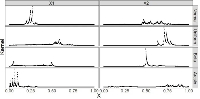
Figure 1.5 Unnormalized joint posterior distribution ofγ1 andγ2 when k= 2 for data from four different distributions withn= 50. . . 25
Figure 1.6 Unnormalized marginal posterior densities for γ1 and γ2 when k= 2 based on data from four different distributions withn= 50. . . 27
Figure 1.7 Example of the unnormalized full conditional distribution of an individualγj. 29
Figure 1.8 A demonstration of the bounding function in red,g, used for rejection sam-pling. . . 31
Figure 1.9 Plots demonstrating the PDF”s of distributions used for testing DUOS. . . . 36
Figure 1.10 Trace plots for the cut-points and four of five bin probability parameters are displayed in the first row. The ACF plots with lag=1000 are plotted in the second row for each set of parameters. These figures are based on results from data simulated from the ‘line’ distribution: n= 50. . . 38
Figure 1.11 Three different chains with diverse starting values were overlaid for each set of parameters. This is based on data simulated from the ‘line’ distribution: n = 50. . . 39
Figure 1.12 Trace plots for the cut-points and four of five bin probability parameters are displayed in the first row. The ACF plots with lag=1000 are plotted in the second row for each set of parameters. This is based on data simulated from the ‘line’ distribution: n= 500. . . 40
Figure 1.13 Three different chains with diverse starting values were overlaid for each set of parameters. This is based on data simulated from the ‘line’ distribution: n= 500. . . 41
Figure 1.14 Trace plots for four of the parameters are displayed in the first row when k = 12. The ACF plots with lag=1000 is plotted in the second row for each set of parameters. This is based on data simulated from the ‘line’ distribution: n= 500. . . 42
Figure 1.15 Three different chains with diverse starting values were overlaid for four of each set of parameters with k = 12. This is based on data simulated from the ‘line’ distribution: n = 500. . . 43
Figure 1.17 A comparison of Gibbs posterior simulations from DUOS to the actual marginal posterior distributions for four distributions where n = 50 and k= 2. . . 44
Figure 1.18 LOESS smoothing curves fit to the number of cut-points verses the PSRF for each sample size and distribution. . . 45
Figure 1.19 LOESS smoothing curves fit to the number of cut-points verses the test statistic from the Geweke diagnostic for each sample size and distribution. . 47
Figure 1.20 Plots LOESS smoothing curve fit to the number of cut-points verses the MISE by each sample size and distribution. . . 49
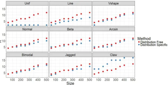
ple size (default for DUOS). The ‘distribution specific’ method is a choice for cut-points based on the size AND distribution. . . 52
Figure 1.23 Plots of LOESS smoothing curves fit to the sample size verses MISE for each distribution and method: DUOS (kbased on table1.1), DPMN, and KDE. 53
Figure 1.24 Plots of the Bayesian density estimate from DUOS for the 9 test distribu-tions: n= 50. . . 54
Figure 1.25 Plots of the Bayesian density estimate from DUOS for the 9 test distribu-tions: n= 400. . . 55
Figure 1.26 Plots of density estimates from DUOS, KDE, and DPMN:n= 400. . . 56
Figure 1.27 Plots a smooth LOESS curve of the sample size verses the MISE on the CDF results for each distribution and methods: DUOS, KDE, and DPMN. . 57
Figure 1.28 Plots of the DUOS Bayesian estimate of the CDF for the 9 test distributions: n= 50. . . 58
Figure 1.29 Plots of the DUOS Bayesian estimate of the CDF for the 9 test distributions: n= 400. . . 59
Figure 1.30 Plots of all CDF estimate from all methods for the 9 test distributions: n= 400. . . 60
Figure 1.31 Plots of the sample size verses the estimate of the mean with the upper and lower bounds of the credible interval. The true value for the mean is at the horizontal red line. . . 63
Figure 1.32 Plots of the sample size verses the estimate of the variance with the upper and lower bounds of the credible interval. The true value for the variance is at the horizontal red line. . . 64
Figure 2.1 A histogram of a sample of data with the grid overlaid in blue and data in red. . . 80
Figure 2.2 A demonstration of how the weights are calculated for the weighted average to estimate the integral. . . 81
Figure 2.3 Plotsy1, ..., ymverses the first row of the prior covariance matrix withs1 = 1 and four different values ofc1: 0.1, 2, 10, and 60. . . 88 Figure 2.5 Convergence plots for data from theN(0,1) distribution: n = 50. The prior
parameters weres1 = 2.15 andc1 = 1. The proposal parameters were s2 = 2.74008 and c2 = 0.5. . . 89 Figure 2.7 Convergence plots for data from the ‘line’ distribution: n= 500. The prior
parameters were s1 = 1 and c1 = 2. The proposal parameters were s2 = 0.0009, andc2 = 1. . . 90 Figure 2.9 Convergence plots for data from the N(0,1) distribution: n = 500. The
prior parameters were s1 = 1 and c1 = 10. The proposal parameters were
s2 = 0.0474264 andc2 = 5. . . 91 Figure 2.10 Plotsc1 verses the ACF for a single parameter at lag 100. A separate LOESS
curve was fit for each value ofs1. . . 92 Figure 2.11 Plotsc1 verses the mean Geweke statistic. A separate LOESS curve was fit
for each value ofs1. . . 93 Figure 2.12 Plotsc1 verses the MISE. A separate LOESS curve was fit for each value of
s1. . . 95 Figure 2.13 LOESS curves fit to the sample size verses a variety of statistical summaries
on the PSRFs. . . 97
Figure 2.14 Plots of the sample size verses MISE for GOLD compared to DUOS, DPMN, and KDE. . . 98
400. The prior parameters were set to s1 = 1.10 and c1 = 8, the proposal correlation parameter was set to c2 = 4, and s2 is chosen by the Graves method. . . 101
Figure 2.17 Plots of the density estimates from GOLD and DUOS for all distributions: n = 400. For GOLD, s1 = 1.10, c1 = 8, c2 = 4, and s2 is chosen by the Graves method. For DUOS, the number of cut-points was set tok= 11. . . 102
Figure 2.18 Plots of the sample size verses MISE on the CDF from GOLD compared to DUOS, DPMN, and KDE. . . 104
Figure 2.19 Plots of the CDF estimates from GOLD for all test distributions: n = 50. The prior parameters were set to s1 = 1.10 and c1 = 8, the proposal correlation parameter was set to c2 = 4, and s2 was chosen by the Graves method. . . 105
Figure 2.20 Plots of the CDF estimates from GOLD for all test distributions: n = 400. The prior parameters were set to s1 = 1.10 and c1 = 8, the proposal correlation parameter was set to c2 = 4, and s2 was chosen by the Graves method. . . 106
Figure 2.21 Plots of the size of the data set verses the estimate of the mean with the upper and lower bounds of the credible interval. The actual value for the mean is represented by a horizontal red line. . . 110
Figure 2.22 Plots of the size of the data set verses the estimate of the variance with the upper and lower bounds of the credible interval. The actual value for the variance is represented by a horizontal red line. . . 111
Figure 3.2 The test distributions used to demonstrate the functions to implement DUOS and GOLD and analyze the output. . . 118
Figure 3.3 Histograms of data simulated from four of the test distributions. . . 122
Figure 3.4 Trace plots for 4 cut-points overlaid on a single graph for the output from
duos on the unif(0,1) data: n= 50. . . 132
Figure 3.6 Trace plots for 5 cut-points overlaid on a single graph for the output from
duos on the N(0,1) data: n = 100. Compares two different ways to scale the data between 0 and 1. . . 134
Figure 3.7 Running mean plots for 15 cut-points overlaid on a single graph for the output fromduos on the‘claw’ data: n= 400. . . 135
Figure 3.9 ACF plots for 8 cut-points overlaid on a single graph for the output from
duos on ‘trimodal’ data: n= 200. Compares the default alpha to an more informedalpha. . . 136
Figure 3.10 ACF plots for 4 cut-points overlaid on a single graph for the output from
duos on the unif(0,1) data: n= 50. . . 137
Figure 3.12 Running means for 6 bin probabilities overlaid on a single graph for theduos
output on theN(0,1) data: n= 100. Compares two different ways to scale the data between 0 and 1. . . 138
Figure 3.14 Running mean plots for 9 bin probabilities overlaid on a single graph for the output from duos on the ‘trimodal’ data: n = 200. Compares the default
alpha to an informative alpha. . . 139
Figure 3.15 ACF plots for the 16 bin probabilities overlaid on a single graph for the output fromduos on the ‘claw’ data: n= 400. . . 140
Figure 3.16 Trace plots for the 5 bin probabilities on separate graphs for theduos output on the unif(0,1) data: n= 50. . . 141
the duos output on the ‘trimodal’ data: n = 200. Compares the default
alpha to a more informativealpha. . . 143
Figure 3.21 Trace plots for the first 6 of 15 cut-points on separate graphs from duos
output on the ‘claw’ data: n= 500. . . 144
Figure 3.23 Running mean plots for 6 of the 15 cut-points on individual graphs from the
duos output on the ‘claw’ data: n= 500. Compares the results from only 20,000 iterations to 50,000 iterations. . . 145
Figure 3.25 Trace plots for 6 of the 7 cut-points on individual graphs fromduosoutput on the ‘trimodal’ data: n= 200. Compares the defaultalpha to an informative
alpha. . . 146
Figure 3.26 The histograms of the posterior draws for the cut-points from the duos
output compared to their priors for data fromunif(0,1): n= 50. . . 148
Figure 3.28 Posterior verses prior plots for 5 cut-points from the duos output on the N(0,1) data: n = 100. Compares two different ways to scale the data between 0 and 1. . . 149
Figure 3.30 Posterior verses prior plots for 6 of 8 bin probabilities from the duos out-put on the ‘trimodal’ data: n = 200. Compares the default ‘alpha’ to an informative ‘alpha’. . . 150
Figure 3.32 Posterior verses prior plots for 6 of the 15 cut-points fromduos output on the ‘claw’ data: n= 500. Compare 20,000 iterations to 50,000 iterations. . . 152
Figure 3.35 The Bayesian estimate of the PDF on data simulated from theN(0,1) dis-tribution: n= 100. Compares the results with default scaling to alternative scaling. . . 154
Figure 3.36 The Bayesian estimate of the PDF based on data simulated from the ‘tri-modal’ distribution: n= 200. . . 155
Figure 3.38 The Bayesian estimate of the CDF on data simulated from the unif(0,1) distribution withn= 50 and theN(0,1) distribution with n= 100. . . 156
Figure 3.40 The posterior mean and median estimate of the density on the unif(0,1) distribution: n= 50. . . 157
Figure 3.41 The Bayesian estimate of the PDF on data simulated from from‘claw’: n = 500. 20,000 iterations were discarded for calculating the estimate. . . 158
Figure 3.43 The posterior mean estimates of the PDF with credible intervals on data simulated fromunif(0,1) withn= 50 and N(0,1) withn= 100. . . 159
Figure 3.45 The posterior mean estimates of the CDF with credible intervals on data simulated from the ‘trimodal’ distribution with n = 200 and the ‘claw’ distribution withn= 400. . . 160
Figure 3.46 The posterior mean estimates of the PDF with histograms of the samples on data simulated from unif(0,1) with n = 50, N(0,1) with n = 100, ‘trimodal’ withn= 200, and ‘claw’ with n= 500. . . 161
Figure 3.47 The Bayesian estimates of the CDF with the ECDF of the samples on data simulated from unif(0,1) with n = 50, N(0,1) with n = 100, ‘trimodal’ withn= 200, and ‘claw’ with n= 500. . . 163
Figure 3.48 The posterior median estimate of the PDF with the credible intervals and histogram of the sample data simulated from N(0,1): n = 100. . . 164
Figure 3.49 The posterior median estimate of the CDF with the credible intervals and ECDF of the sample data simulated from unif(0,1): n = 50. . . 165
Figure 3.52 An interactive plot of the posterior mean estimate of the PDF, credible intervals, and histogram of the data simulated from theN(0,1) distribution:
n= 100. . . 168
Figure 3.53 The Bayesian estimate of the CDF on data simulated from the ‘claw’: n = 500 in an interactive graph. . . 169
Figure 3.54 The posterior draws for the estimate of the density at (0.2, 0.4, 0.6, 0.8) for the data from unif(0, 1): n = 50. . . 173
Figure 3.55 A variety of convergence plots created on the simulations of the posterior density at 1.926 for the ‘trimodal’ data: n= 200. . . 175
Figure 3.56 Histograms of the posterior estimate of the probabilities of being in each mode based on the ‘claw’ data: n= 400. . . 182
Figure 3.57 The histogram of the posterior simulations for the expectation of the density estimate on theunif(0,1) data: n= 50. . . 185
Figure 3.58 The posterior mean densities from DUOS on samples of size 250. . . 189
Figure 3.59 The posterior mean CDFs from DUOS on samples of size 250. . . 191
Figure 3.60 Histograms of data simulated from four of the test distributions. . . 195
Figure 3.61 Histogram of the posterior samples for unnormalized log density at a 4 dif-ferent locations. . . 205
Figure 3.62 Trace plots for the output fromgold on the unif(0,1) data: n= 50. . . 206
Figure 3.63 Trace plots for the output fromgold on the N(0,1) data: n= 100. . . 207
Figure 3.64 Running means for the output fromgold on the N(0,1) data: n= 100. . . . 208
Figure 3.67 Running mean plots for 12 parameters from gold on the ‘bimodal’ data: n= 400. . . 210
Figure 3.68 ACF plots for parameters fromgold on the unif(0,1) data: n= 50. . . 211
Figure 3.69 ACF plots for parameters fromgold on the exp(1) data: n= 200. . . 212
Figure 3.70 Trace plots of the last 20,000 iterations for 6 parameters from thegold output on the ‘bimodal’ data: n= 400. . . 213
Figure 3.72 Trace plots and ACF plots fromgold on thebeta(2,5) data: n= 500. . . 214
Figure 3.73 Posterior verses prior plots for the results from gold on theunif(0,1) data: n= 50. . . 216
Figure 3.74 Posterior verses prior plots for the results fromgold on the ‘bimodal’ data: n= 400. . . 217
Figure 3.76 Posterior verses prior plots for the npar = 10 parameters requested from
gold on the N(0,1) data: n= 100. . . 218
Figure 3.77 Posterior verses prior plots for the results from gold on the exp(1) data: n= 200. . . 219
Figure 3.78 Posterior verses prior plots for the results from gold on thebeta(2,5) data: n= 500. . . 220
Figure 3.79 The Bayesian estimate of the PDF on data simulated from fromN(0,1): n = 100. . . 221
Figure 3.80 The Bayesian estimate of the CDF on data simulated from unif(0,1): n = 50.222
Figure 3.81 The Bayesian estimate of the PDF on data simulated from theexp(1) data : n = 200. A burnin of 5,000 iterations were discarded for calculating the estimate. . . 223
Figure 3.82 The Bayesian estimates of the PDF or CDF on data simulated fromunif(0,1) withn= 50, ‘bimodal’ withn= 400,exp(1) withn= 200, andN(0,1) with n= 100. . . 224
from unif(0,1) with n = 50, N(0,1) with n = 100, exp(1) with n= 200, and ‘bimodal’ withn= 400. . . 226
Figure 3.86 The Bayesian estimates of the PDF and CDF with the credible intervals and histogram or ECDF of the sample on data simulated from ‘bimodal’: n= 400.227
Figure 3.87 The interactive Bayesian estimate of the CDF on data simulated from the N(0,1) data: n= 100. . . 228
Figure 3.88 The interactive Bayesian estimate of the PDF on data simulated from the unif(0,1) data: n= 50. . . 229
Figure 3.89 The interactive Bayesian estimate of the CDF and credible intervals on data simulated from the ‘bimodal’ data: n= 100. . . 230
Figure 3.90 The interactive Bayesian estimate of the CDF on data simulated from the exp(1) data: n= 200. . . 231
Figure 3.91 The posterior draws for the estimate of the density at (-2.111, 1.153, 6.234) for the ‘bimodal’ data: n= 400. . . 235
Figure 3.92 The posterior draws for the estimate of the CDF for P(x< -0.52) and P(x >4) on the ‘bimodal’ data: n= 400. . . 241
Figure 3.93 A histogram of the posterior simulations for the expectation of the estimated density on theN(0,1) data: n= 100. . . 245
Figure 3.94 The posterior mean densities from GOLD on all test distributions: n= 250. 247
Figure 3.95 The posterior mean CDF estimates from GOLD on all test distributions: n= 250. . . 248
Figure B.1 Plots of the trace plots for four cut-point parameters for results from DUOS on all distributions withk= 4: n= 50. . . 266
Figure B.2 Plots of the trace plots for four of the five bin probability parameters for results from DUOS on all distributions with k= 4: n= 50. . . 267
Figure B.3 Plots of the overlaid chains with diverse starting values on trace plots for the cut-point parameters for results from DUOS on all distributions with k= 4: n = 50. . . 267
Figure B.4 Plots of the overlaid chains with diverse starting values on trace plots for the cut-point parameters for results from DUOS on all distributions with k= 10: n = 50. . . 268
Figure B.5 Plots of the trace plots for four cut-point parameters for results from DUOS on all distributions withk= 4: n= 500. . . 268
Figure B.6 Plots of the trace plots for four of the five bin probability parameters for results from DUOS on all distributions with k= 4: n= 500. . . 269
Figure B.7 Plots of the overlaid chains with diverse starting values on trace plots for the cut-point parameters for results from DUOS on all distributions with k= 4: n = 500. . . 269
Figure B.8 Plots of the trace plots for four of the cut-point parameters for results from DUOS on all distributions withk= 12: n= 500. . . 270
Figure B.9 Plots of the trace plots for four of the bin probability parameters for results from DUOS on all distributions with k= 12: n= 500. . . 270
Figure B.10 Plots of the overlaid chains with diverse starting values on trace plots for the cut-point parameters for results from DUOS on all distributions with k= 12: n = 500. . . 271
Figure B.11 Plots of the ACF plots for four cut-point parameters for results from DUOS on all distributions: n = 50. . . 271
Figure B.12 Plots of the ACF plots for four of the five bin probability parameters for results from DUOS on all distributions: n = 50. . . 272
Figure B.15 Running mean plots for k = 4 cut-points and 4 of the 5 bin probability parameters on the ’line’ data: n = 50. . . 273
Figure B.16 Running mean plots for k = 4 cut-points and 4 of the 5 bin probability parameters on the ’line’ data: n = 500. . . 274
Figure B.17 Running mean plots for 4 of thek = 12 cut-points and 4 of bin probability parameters on the ’line’ data: n = 500.. . . 275
Figure B.18 Comparing histograms of posterior simulations from the cut-points with k= 2 to the true unnormalized marginal densities for these same parameters for samples of size 50. . . 276
Figure B.19 Comparing histograms of posterior simulations from the cut-points with k= 2 to the true unnormalized marginal densities for these same parameters for samples of size 500. . . 276
Figure B.21 A comparison of Gibbs posterior simulations from DUOS to the actual marginal posterior distributions for five distributions where n = 50 andk= 2.277
Figure B.22 Plots of the sample size verses the MSE for each distribution for four different methods: DUOS1 (cut-point choice specific to size and distribution), DUOS2 (DUOS with the number of cutpoints based on table 1.1 determined by size, but not Distribution, DUOS3 (10 cut-points for all examples)), DPMN (Dirichlet Process Mixture of Normals), KDE1 (kernel density estimation using ’nrdo’), and KDE2 (kernel density estimation using ’SJ’) . . . 277
Figure B.23 Trace plots for data of size 50 from all distributions from GOLD output: s1 = 1,c1 = 2,c2 = 1, ands2 chosen by the Graves algorithm. . . 278
Figure B.24 Trace plots for data of size 500 from all distributions from GOLD output: s1 = 1,c1 = 2,c2 = 1, ands2 chosen by the Graves algorithm. . . 278 Figure B.25 ACF plots for data of size 500 from all distributions from GOLD output: s1
= 1,c1 = 10,c2 = 5, ands2 chosen by the Graves algorithm. . . 279 Figure B.26 ACF plots for data of size 50 from all distributions from GOLD output: s1
= 1,c1 = 2,c2 = 1, ands2 chosen by the Graves algorithm. . . 279 Figure B.27 ACF plots for data of size 500 from all distributions from GOLD output: s1
= 1,c1 = 2,c2 = 1, ands2 chosen by the Graves algorithm. . . 280 Figure B.28 ACF plots for data of size 500 from all distributions from GOLD output: s1
= 1,c1 = 10,c2 = 5, ands2 chosen by the Graves algorithm. . . 280 Figure B.29 Plots of the sample size verses the estimate of the median with the upper
and lower bounds of the credible interval. The true value for the median is at the horizontal red line. . . 281
Figure B.30 Plots of the sample size verses the estimate of the median from GOLD with the upper and lower bounds of the credible interval. The true value for the median is at the horizontal red line. . . 282
I want to thank Dr. Vardeman and Dr. Nordman for their help and guidance and dedicating their time to be my advisors. I also want to thank my committee and other teachers I have had who provided a wonderful education during my time at Iowa State. I offer a final thank to all my family members and friends who provided encouragement and long talks on the phone whenever I needed them.
ABSTRACT
Density estimation is a standard tool for investigating attributes of a continuous distribution assumed to have generated a finite sample of data. Performing density estimation in a Bayesian framework allows for prior information about the underlying distribution to be used in the esti-mation. However, unless the size of the sample is very small, it is typically not desirable for the prior information to overwhelm information provided by the sample. Under consideration are Bayes methods for univariate density estimators on (0,1), where prior information does not dominate the outcome, and the resulting estimates are flexible and not constrained to belong to any standard parametric class of densities. The first method, referred to as DUOS, is based on a Distribution
of Uniform Order Statistics prior. DUOS uses a class of step functions with a prior on the bin endpoints to allow for random bin widths and locations. The second method is called GOLD which applies a Gaussian Process on a pre-Log-Density to a class of continuous functions. A full inves-tigation of each Bayes density estimator is presented, including the use of Markov Chain Monte Carlo to simulate from the posterior distributions, inference on the results, and extensive simula-tion studies establishing their competitiveness with other methods. These simulasimula-tion studies also functioned as a guide to the development of defaults for the prior parameters. Finally, the package
biRdinR(R Core Team (2017)) provides the functions necessary to implement both methods and completely assess the Bayesian estimates of the density, the cumulative distribution function, and a variety of statistical summaries of the density estimate.
1.1 Introduction
Density estimation has long been applied as the primary means of assessing various properties of data sets. Due to the continued importance in understanding the underlying distributions of random variables, it has been described as a “fundamental concept” by Silverman, B. (1998). The histogram is one of the earliest forms of visually estimating a density. The use and development of histograms was seen throughout the mid to late 1800’s (Pearson, K. (1895); Friendly, M. (2005)) and possibly as early as the 1600’s (Westergaard, H. (1968)).
Even though the histogram is the oldest density estimator according to Scott, D., Tapia, R., and Thompson, J. (1977) and (Silverman, B. , 1998, p. 7), it is also among the most extensively applied (Wegman, E. , 1972; Silverman, B. , 1998, p. 7). In fact, it is introduced to students early on in their education as a means of density estimation (Friel, S., Curcio, F., and Bright, G. (2001)) and continues to be taught throughout college today. Outside of academia, the histogram is often used in news outlets as a means of displaying data. This is most likely due to the clarity it provides in explaining the overall picture of the data to those outside of mathematics and statistics fields as stated by (Silverman, B. , 1998, p. 5). Although the histogram is useful for quickly assessing basic aspects of the data, it has several disadvantages, one of them being its lack of smoothness and discontinuities (Gramacki, A. , 2018, p. 8-10). The appearance of the distribution displayed by the histogram also depends heavily on the number of bins, the bin widths, and positioning of the first bin (Gramacki, A. , 2018, p. 8-10). It also cannot estimate the density outside the range of the data as pointed out by Scott, D., Tapia, R., and Thompson, J. (1977). Thus, many different statistical techniques for estimating a density have been and still are being developed.
These density estimates have spread far beyond the histogram in both frequentist and Bayesian statistics. This does not negate the usefulness of the histogram. A simple density estimate can
be useful for presenting various properties of a data set such as multiple modes or skewness. It is also useful for presenting the data back to the client in an understandable manner (Silverman, B. , 1998, p. 5). With the advancement of methods in density estimation, its uses have grown as well. Parzen, E. (1962) mentions using density estimation to estimate hazard (or conditional rate of failure) f(x)/(1-F(x)). The uses of a density estimate extends to an even wider range of methods from discriminant analysis (Fix, E. and Hodges, J. (1989)) and anomaly detection (Pimental, M., Clifton, D, Clifton, L., and Tarassenko, L. (2014)) to applications in bio-assay, regression (Antoniak, C. (1974)) and machine learning (Sugiyama, M., Suzuki, T., and Kanamori, T. (2012)) to name a few.
The focus of the research discussed in Chapters 1 and 2 is the use of Bayesian techniques to produce density estimates without being limited to any standard parametric class of densities. Any further reference to nonparametric Bayesian density estimation is not regarding Bayesian analysis with an infinite number of parameters, although the number of parameters in both presented density estimators is not fixed and can be quite large. The exact number of unknown parameters for the methods in Chapters 1 and 2 is finite, but can fluctuate depending on prior specifications or the size of the data. The advantages of this ‘nonparametric’ approach is that no knowledge is required about the underlying density assumed to have generated the data of interest. Another reason to use nonparametric density estimation as opposed to parametric, according to Gramacki, A. (2018), is “All of the classical parametric densities are unimodal...whereas a number of practical problems involve multimodal densities, making the parametric density estimation unfit for many applications.” Other advantages of Bayesian methods in particular are the ability to include prior information (Leonard, T. (1973)) and the fact that Bayesian methods do not rely on “large sample justification” (Ferguson, T. (1983)).
Although the priors of the proposed methods can be modified to include influential prior in-formation, they are designed to produce results that are dominated by information from the data rather than the priors. These priors and a guide to default prior parameters suggested by a large
Due to the vast area of research concerning density estimation, the following literature review concentrates on nonparametric density estimation. These density estimators are nonparametric in the sense that results are not confined to a specific class of densities. Thus, approaches assuming the data is drawn from a standard parametric family of distributions, using maximum likelihood or a Bayesian approach to estimate the parameters, are not considered. Specific emphasis is placed either on popular nonparametric methods that produce a baseline for comparison or share similarities to the proposed methods.
1.1.1.1 Non-Bayesian Density Estimation
The focus of this section is on the non-Bayesian literature concerning key stages in the devel-opment of nonparametric density estimation. Particular emphasis is placed on the kernel density estimate (KDE), given that it is the most commonly used density estimator after the histogram (Silverman, B. , 1998, p. 17; Gramacki, A. , 2018, p. 3). In order to assess the overall performance of the methods in Chapters 2and 3, results are compared to the kernel density estimator.
Work in nonparametric density estimation began in the late 1800’s. According to Wegman, E. (1972), who surveyed available nonparametric density estimation methods, the first attempt at probability density estimation besides the histogram was most likely the Pearsonian system of densities (Pearson, K. (1895)). In Pearson, K. (1902a) the subject of the paper was not density estimation specifically, but the concept of estimating a set of unknown parameters for a known curve form betweeny andx. In Pearson, K. (1902b), this idea was extended to densities in which data for part of the density is known. He specifically discussed executing this concept when the known curve is normal.
Other early work in the area of nonparametric density estimation was in 1951 (Fix, E. and Hodges, J. (1989)). The authors proposed a method for density estimation to use in discriminant analysis that does not assume any standard parametric forms on the underlying densities. Their goal was - given a new data pointz - to answer the question: doesz come from distributionf org? Their idea was to use the proportion of data in a small neighborhood ofz to estimate the probability. Advantages of this method include that it is easily extended to more than two populations and that this method is consistent with the likelihood ratio if the distribution is known. However, the consistency results are not as reliable when the sample size from either distributionf org is small. The primary obstacle in this method is choosing the width of the neighborhoods. Regions that are too small or too large result in bad approximations. Another issue arises if there are few data points near the z in question.
The earliest forms that led to kernel density estimation were developed by Rosenblatt, M. (1956). He continued to expand nonparametric density estimation by introducing an estimator similar in form to Fix, E. and Hodges, J. (1989), except specifically focusing on density estimation:
ˆ fn(x) =
# of sample points in (x−hn, x+hn)
2nhn
(1.1) wherehn is a function of the sample sizen, and hn → 0 asn → ∞.
Rosenblatt introduced the idea of other kernels, but Parzen, E. (1962) fully developed the use of the kernel in density estimation. The main purpose of this work was to propose a method to estimate a probability density and its mode. The approach was motivated by a comparable problem of working with stationary time series data to estimate the spectral density function (Parzen, E. (1962)). Parzen proposed the classical form of the kernel density estimator seen in Equation 1.2 when trying to study the properties of the form in Equation 1.1. Note that fn(x) is
the authors notation for an estimate of f:
fn(x) = 1 nh n X j=1 K x−Xj h (1.2)
sample sizes, and this method does not require a large sample size. However, he pointed out, and Wegman, E. (1972) confirmed, that the properties of the kernel density estimate depend onh and K(y). Parzen did not directly recommend any of the kernels, but he did point out what value of h minimizes the mean square error for a givenK(y). However, this is only when the form of the true density, f(x) is known. Thus, the primary challenge with this method is choosing the appropriate bandwidth parameter once a suitable kernel is selected.
One of the primary advantages of KDE mentioned above is the smoothness of the result (Sil-verman, B. , 1998, p. 13). Silverman also discussed one of the main disadvantages of KDE, which is that noise often appears in long-tailed distributions unless the density estimate is over smoothed (Silverman, B. , 1998, p. 18). However, there are variable kernel methods created to help with this by allowing the bandwidth to be non-constant (Silverman, B. , 1998, p. 21).
As stated earlier, since kernel density estimation continues to remain the most popular choice for nonparametric density estimation (Aitkin, M. , 2009, p. 458), it is used to measure performance in the results in Sections 1.3.2and2.4.2. Its popularity is most likely due to its ease of implemen-tation and variety of applications including discriminant analysis, cluster analysis, regression, and multidimensional statistical process control (Gramacki, A. , 2018, p. 5). In order to use kernel density estimation, it is necessary to choose a kernel and a bandwidth.
According to (Gramacki, A. , 2018, p. 25) and (Aitkin, M. , 2009, p. 458), the Gaussian kernel is a common choice. This is even though (Scott, D. , 2014, p. 145) determined that it is the bandwidth that primarily influences the results, not the kernel. (Aitkin, M. , 2009, p. 458) confirmed this, and (Silverman, B. , 1998, p. 43) showed there is not much difference between kernels in terms of the mean integrated squared error. Therefore, all results presented from a kernel density estimator in Sections 1.3.2and 2.4.2use the standard normal kernel.
There is not a simple solution for choosing the bandwidth, but there is a considerable amount of research related to this area (Gramacki, A. , 2018, p. 29). Different situations warrant varying estimations for the bandwidth. The bandwidth could be picked and modified based on visualizing the results. But as (Silverman, B. , 1998, p. 43-44) points out, users of the KDE may want automation of the bandwidth choice due to lack of knowledge or because of having to apply KDE numerous times makes it advantageous to have the bandwidth automatically chosen.
Given that Section 1.3 comprises the analysis of over 1000 simulated data sets, and the desire here is to compare a default application of the method discussed in Section 1.2 to a default for KDE, an automatic choice of the bandwidth parameter is preferable. The default in the function
density inR, is from (Silverman, B. , 1998, p. 48), and is given in Equation 1.3:
h= 0.9An−1/5 (1.3)
TheAin equation1.3ismin
sd(y),IQR1.34(y)
where IQR is the interquartile range. This method is easy to apply and works well over a diverse set of densities (Silverman, B. , 1998, p. 48). The h in equation 1.3 has also been stated as either a ‘rule-of-thumb’ or ‘reasonable initial choice’ by (Gramacki, A. , 2018, p. 65) and Scott, D. (2014). According to a sensitivity analysis, as long as h is within 15 to 20 % of the optimal h∗, h is generally satisfactory (Scott, D. , 2014, p. 172). The one drawback of this choice is that it does tend to over smooth in some cases, but some have proposed that a bandwidth calculator that tends to over smooth should be the estimator of choice (Terrell, G. (1990)). Therefore, results from KDE use the bandwidth described in equation1.3.
1.1.1.2 Bayesian Density Estimation
The purpose of this section is the development of Bayesian density estimation with a focus on density estimators similar to that presented in Section 1.2. A non-Bayesian choice for comparison has already been made in the form of the kernel density estimator. Thus, a secondary focus of this section is the evolution of a common Bayesian density estimator. This will establish a means of assessing the performance of the method in Section 1.2.
ˆ
f(x) = wx(y)dn(y) = j
wx(xj)/N (1.4)
wheren(y) is the proportion of observations less thanyandwx(y) is a weighting function regulated
by an optimality criterion (Whittle, P. (1958)). He suggested working with the unnormalized density - ϕ(x) = M f(x) - when the sample size is not predetermined, which is still given the form in Equation 1.4. This method is semi-Bayesian since ϕ(x) or f(x) is assumed to come from some family of curves, thus, incorporating prior knowledge about the shape of the density. Values for ˆϕ(x) or ˆf(x) are then obtained through optimization. Although results show invariance to transformation, this method has a disadvantage, pointed out by Dickey, J. (1968) and Leonard, T. (1973), in that the estimate of the underlying distribution can result in negative values.
Another early reference to Bayesian density estimation was in the work of Good, I., and Gaskins, R. (1971). They carried on the work in smooth density estimates by working with the log-likelihood. Rather than working directly with the maximum likelihood, a roughness penalty is subtracted from the log-likelihood. If maximum likelihood is applied directly to the likelihood, “Nobody accepts this solution because it is too rough” (Good, I., and Gaskins, R. (1971)). Thus, the authors work instead with:
w(f) =X
i
logf(xi)−Φ(f) (1.5)
where Φ is a functional of f. If a fully Bayesian analysis were implemented, the prior on this space would be proportional to e−Φ. For this method, some sort of density function is assumed in the functional. Although a fully Bayesian approach to this is discussed - given interpretations resulting in directly comparing assumed density functions - full results are based on the frequentist version. This is due to the complicated nature of accounting for potentially misclassifying the true
underlying density in Φ(f) . Also, if a Bayesian route were taken, Leonard, T. (1978) points out that it is unclear how prior information is incorporated in the choice of a roughness penalty.
One of the methods that shares a somewhat similar approach to that proposed in Section1.2is the work of Leonard, T. (1973). He implemented a fully Bayesian analysis which does not assume any form for the underlying density. He stated: “A weakness of the Bayesian approach has been its inability to cope with independent observations whose common distribution is not restricted to any particular family” (Leonard, T. (1973)). Assume n observations are independent and identically distributed according to an unknown densityq(y). He chose a histogram approach in that data is divided into sbins of equal width W. Let Ij represent the bins whereIj = (ζj −12W,;ζj +12W].
The midpoints areζ1, ..., ζs such thatζj+1−ζj =W. Thus, the densityq(y) is estimated from the
form in Equation1.6:
q∗(y) =W−1θj, y∈ζj (1.6)
whereθj is the probability associated with thejthbin. The prior on theθ’s allows prior information
about the smoothness ofq(y) to be incorporated into the results. A prior is not directly placed on the θ’s, but rather to the log of the θ’s so that the resulting parameters are on the real number line. The addition of theD(γ) in Equation 1.7is to ensure that theθ’s sum to one.
γj =logθj +D(γ),(j= 1, ..., s)
D(γ) =log(X
g
eγg) (1.7)
A prior is not directly applied toγ. Instead, the form,γ =ηκ+β, is used in order to streamline results without effectingθ. κis ansx 1 vector containing all 1’s. Sinceθj =eβj/Pgeβg, the choice
of prior for κ does not influence θ. Leonard chose the uniform prior over the whole real line as the prior, and assumed η is independent of β. The key here is that a multivariate normal prior is placed on β. The mean µ is chosen so that P
where 0< σ2 <∞ and −1 < ρ <1. This resulting density estimate is nonnegative and Leonard, T. (1973) states that the method is “fairly flexible” in providing a way to integrate information about the smoothness and shape of the density into the prior. However, it may be difficult to choose this information if little is known about the underlying distribution. This method offers a solution by allowing for the placement of priors on the variance and covariance parameters, but the choice of prior mean vector needs to be carefully considered due to its influence on the results.
One of the common Bayesian density estimators used today began with the work of Ferguson in developing the Dirichlet process (Ferguson, T. (1973)). Ferguson specifically addressed the use of Bayesian in nonparametric problems: “The Bayesian approach to statistical problems, though fruitful in many ways, has been rather unsuccessful in treating non-parametric problems” (Ferguson, T. (1973)). Ferguson’s goal in developing Dirichlet process priors was to create a prior that had large support and resulted in a posterior with an analytical solution. Full details of the Dirichlet process can be found in Ferguson, T. (1973). The basics are given below since this concept is used in a density estimator for comparative purposes later on.
Definition 1.1.1. Dirichlet Process: Let H be a space and A be a σ-field of subsets, and let α be a finite non-null measure on (H, A). Then a stochastic process P indexed by elements A of
A, is said to be a Dirichlet process on (H,A) with parameter α if for any measurable partition (A1, ..., Ak) ofH, the random vector (P(A1), ..., P(Ak)) has a Dirichlet distribution with parameter
(α(A1), ..., α(Ak)) Ferguson, T. (1973)).
Results in the paper show that if X1, ...Xn is a sample from P, than P|(X1, ..., Xn) is also a
Dirichlet process. Once a Bayes rule is developed, he proceeds to demonstrate how this Dirichlet prior can be used to estimate the distribution function, mean, variance, and other statistics.
Antoniak, C. (1974) stated the following reason for expanding the Dirichlet process to a mixture of Dirichlet processes: “the basic Dirichlet process defined above does not encompass enough of the situations encountered in Bayesian analysis.” He pointed out that the Dirichlet process developed by Ferguson does not always result in the posterior distribution that is a Dirichlet process. Specifically, if sampling from a mixing distribution, the posterior is not a Dirichlet process, but rather a mixture of Dirichlet processes. What makes a mixture of Dirichlet processes is that the measureαdescribed by Ferguson, T. (1973) is now random.
Definition 1.1.2. Mixture of Dirichlet Processes: Let (Θ,A) be a measurable space, let (U,B, H) be a probability space, called the index space, and let α be a transition measure on U X A. We sayP is a mixture of Dirichlet processes on (Θ,A) with mixing distributionH on the index space (U,B), and transition measure α, if for allk = 1,... and any measurable partitionA1, A2, ..., Ak of
Θ we have
P{P(A1)≤y1, ..., P(AK)≤yk}=
Z
u
D(y1, ..., yk|α(u, A1), ..., α(u, Ak))dH(u) (1.9)
whereD(θ1, ..., θk|α1, ...αk) denotes the distribution function of the Dirichlet distribution with
pa-rameters (α1, ..., αk) Antoniak, C. (1974).
Like Ferguson, he proceeds to show that if the prior is a mixture of Dirichlet processes, the posterior is as well. Antoniak demonstrated a variety of applications of mixtures of Dirichlet processes in regression, bio-assay, and discrimination problems.
In 1983, Ferguson took the idea of mixtures and proposed density estimation by mixtures of normal distributions which uses a(Dirichlet process (Ferguson, T. (1983)). Parameters in the model included the means and variances of a countable number of normal distributions and the weights on the normal distributions.
f(x) = ∞
X
i=1
pih(x|µi, σi) (1.10)
whereh(x|µi, σi)≈N(µi, σi). Thus, the parameters in need of estimates are the countably infinite
whereG is the probability measure on the half-plane (µ, σ): σ >0 that gives mass pi to the point
(µi,σi),i= 1,2, ...(Ferguson, T. (1983)). Gis identifiable ifGis confined to be from the collection
of finite probability measures.
For the priors, he assumed (p1, p2, ...) and (µ1, µ2, ..., σ1, σ2, ...) are independent. A set of pa-rameters, q1, q2, ... is assumed to be iid where qi ∼ Beta(M,1). The p1, p2, ... are obtained from these by p1= 1−q1,p2=q1(1−q2),...,pj = Qj−1 i=1qi (1−qj), ....
The pairs (µ1, σ1),(µ2, σ2), ...are assumed to be iidaccording to the gamma-normal conjugate prior where σ12 i ∼Gamma(α,2/β) and µi|σ12 i ∼N(µ,p21 iτ2 ).
One of the interpretations that Ferguson gives for the prior parameter M for the q1, q2, ... is that small values indicated little prior knowledge, and results are primarily dictated from the data. Large values of M indicated more confidence in the prior information. M also expresses prior beliefs about the sizes of the probabilities.
Under this prior for (p1, p2, ..., µ1, µ2, ..., σ1, σ2, ...), the distribution of G is a Dirichlet process with α = M G0. M is the prior parameter for q1, q2, ... and G0 is the conjugate prior for (µ, σ2). The author proceeds with a Monte Carlo approach to implement this algorithm, demonstrating examples on very small sample sizes.
Escobar, M. and West, M. (1995) continued to extend this idea of using mixtures of Dirichlet processes through situations where the data is also modeled using mixtures of normal distributions. Given the work in MCMC algorithms at this point, they were able to use a Gibbs sampler to simulate from the posterior distribution.
Their set up is similar to Ferguson, T. (1983). AssumeY1, ...Yn are conditionally independent.
whereπi= (µi, Vi): i= 1,...,n.
Assume πi come from some prior distribution:
πi ∼G(·)onRXR+ .
ModelG(·) as a Dirichlet process:
G∼D(αG0)
where α is a positive scalar and G0(·) is a bivariate distribution on R X R+ that is the prior expectation of G(·).
The Dirichlet process mixture of normals (DPMN) is a popular method for Bayesian density estimation according to ( ¨Uhwirth-Schnatter, S. et al. , 2015, p. 4). This is most likely due to the ability of the DPMN to adapt to a wide range of distributions (Rossi, P., Allenby, G., and Mcculloch, R. , 2011, p. 79; Christensen, R. , 2011, p. 386).
Given that the DPMN is a popular choice for nonparametric density estimation, it is chosen as the Bayesian version of density estimation to assess the results of the proposed density estimators in Chapters 1 and 2. The method presented by Escobar and West is implemented in DPpackage
(Jara, A., et al. (2011)) in R. This package specifies theG0(·) as the conjugate normal-Wishart distribution.
G0 =N(µ|m1,(1/k0)σ)|W(σ|ν1, ψ1) .
The function DP density implements these methods using a Gibbs sampling algorithm using auxiliary parameters (Neal, R.M.. (2000)). The values forα,m1, k0, and ψ1 can be input by the user, or hyperpriors can be placed on some or all of them. For comparison purposes, it makes sense to use the hyperpriors since other methods will be run on some sort of default rather than using individual prior information.
α|a0, b0 ∼Gamma(a0= 1, b0 = 1)
m1|m2, s2 ∼N(m2 =mean(y), s2=var(y))
k0|τ1, τ2∼Gamma(τ1/2 = 0.1, τ2/2 = 1)
ψ1|ν2, ψ2 ∼IW(ν2= 1, ψ2= 0.1∗var(y)))
(1.12)
Thus, rather than expressing prior knowledge through the prior parameters, all of them are random. Of the density estimators presented above, those that work with fully Bayesian techniques re-quire a substantial amount of knowledge either about the underlying density or how a fair number of parameters affects the results. It is necessary to specify a mean function, underlying distribu-tion, or individual values for the mean function for the Gaussian process in the work of Leonard, T. (1973). This was shown in some cases to heavily influence the results and therefore, should be chosen carefully. When working with the Dirichlet process mixture of normals, there are a range of parameters to specify starting with at least four. The path to inference is also not clear for some of the results from these density estimators. Although both of these estimators have the advantage of being smooth, and DPMN is known to be flexible, the method in Section1.2 presents a Bayesian density estimate that is simpler to provide prior information for, while at the same time laying a clear path to inference.
1.2 Methods
The goal for the methods presented in this section is to create a Bayesian density estimator that is straightforward to implement, while at the same time being flexible enough to require little to no adjustments to estimate a variety of underlying distributions. This is achieved by using simple and non-informative priors where a single parameter is the only necessary adjustment. The first method is called DUOS. This is based on aDistribution ofUniformOrder Statistics prior distribution for
the locations of a fixed number of points that define bins in a class of step function probability densities on (0,1).
In the subsequent sections, full details are given on the step functions used to create density estimates and the priors necessary to achieve these estimates. The resulting posterior distribution is explored to understand its form. This leads into the choice of MCMC algorithm which is used to simulate from the posterior distribution. A variety of graphical and statistical means are presented to assess convergence on the simulations resulting from the MCMC algorithm. These results com-bined with the mean integrated squared error (MISE) were collected on a wide range of possible choices effecting the prior in order to supply an effective default. Performance of DUOS using this default is then compared to other popular density estimate techniques, and then the functionality of DUOS is demonstrated through inference on a variety of statistical summaries. Another advan-tage of DUOS is that the posterior mean estimate of the density produced is continuous, unlike the step functions being averaged. Finally, an extension to DUOS is described in the form of a likelihood-ratio.
1.2.1 Introduction
The method introduced as DUOS is a histogram-like density estimate which places priors on the parameters for a class of step functions that are also probability density functions on (0,1). It is similar to Leonard, T. (1973) and Fix, E. and Hodges, J. (1989) in that DUOS uses the concept of bins. In the case of Fix, E. and Hodges, J. (1989), the width is fixed and the midpoint is a new data point at which to estimate the density using proportions (non-Bayesian). The width is also fixed in the work of Leonard, T. (1973), but the midpoints are established before the Bayesian analysis is implemented. The primary difficulty with the methods in Fix, E. and Hodges, J. (1989) and Leonard, T. (1973), and potential other histogram-like methods is choosing the bin width as it highly influences the result. A solution to this leads to the primary difference between DUOS and these methods which is that the endpoints - and therefore the widths - of each bin are random. This results in bins whose widths are different from each other rather then equal. The locations
based on prior knowledge. This is the one and only necessary piece of prior information to include. To increase the ease of use of DUOS, a reasonable default is demonstrated in Section 1.3.2. The positions of the bin end points are referred to as cut-points. These are random and a distribution on unif(0,1) order statistics is applied as a prior. From here on, this prior and method will be referred to as DUOS. There are also bin probabilities which require a prior as well, and are explained in Section1.2.2.
Given a finite set of independent and identically distributed data assumed to be generated from a continuous distribution, a MCMC algorithm is implemented to sample from the posterior distributions of the cut-points and bin probabilities. The resulting Bayesian estimate then ends up being the average of thousands of step functions. This idea is demonstrated in Figure 1.1showing a continuous posterior mean density as the average of many step functions.
Figure 1.1: An example of a Bayesian density estimate (in red) from DUOS as a mean of many step functions (in blue) overlaid over a histogram of the actual data.
The mean posterior density estimate in Figure 1.1is straightforward to calculate once simula-tions for the cut-points and bin probabilities are achieved. A key advantage of DUOS is that the form of the step function explained in Section1.2.2provides reasonable solutions to producing other results such as the CDF, quantiles, means, and variances and credible intervals for these values.
1.2.2 Data Model
This section fully describes the class of step function densities that achieves the results seen in Figure 1.1. A full introduction to the cut-points and bin probabilities previously mentioned in Section1.2.1is also provided which leads into the need for priors.
Let ˜
x =x1, x2, ..., xniid∼f where f is a continuous distribution assumed to have generated the
sample. The form of f is estimated using an alternative density. This density in Equation 1.13
takes the pattern of a step function or histogram. This form is also flexible, allowing adaptation to a wide variety of shapes of data. The idea is to apply Bayesian concepts to this form, thus allowing the data to influence and produce reasonable choices for the cut-points and bin probabilities. By applying Bayesian techniques to these sets of parameters, the estimate of the density becomes an average of step functions and is, therefore, continuous and much smoother than the step function. The two sets of parameters are defined by:
Letγj represent a cut-point where a pair (γj, γj−1) controls the bin width and location of the bin
ˆ f ˜ γ, ˜ π(x) = π2 (γ2−γ1) γ1 ≤x < γ2 π3 (γ3−γ2) γ2 ≤x < γ3 ... ...≤x < ... πk (γk−γk−1) γk−1≤x < γk πk+1 (1−γk) γk≤x <1 (1.13) where
k: the number of cut-points
˜ γ : 0< γ1 < γ2 < ... < γk−1< γk<1 ˜ π:πk≥0 and Pk+1 j=1πj = 1
As seen by the range of possibilities for xin Equation 1.13, DUOS is designed to work on data with support (0,1). However, data with any range can still have DUOS applied by scaling the data properly. Let x∗1, x∗2, ..., x∗n represent the scaled data achieved using the process in Equation 1.14.
x∗i = xi−(min(˜x)−scalelower) max(
˜
x) +scaleupper−(min(
˜
x)−scalelower)
, i= 1,2..., n (1.14) For all results in Section1.3,scalelower andscaleupperwere given the values of 0.000001 so that
the resulting ˜
x∗ ∈ (0,1). However, the idea of the scalelower and scaleupper is to allow the range
of where the density can be estimated to extend slightly beyond the maximum and minimum. See Chapter 3 for applications using alternative scaling. These values should typically be fairly small to avoid over-extrapolating. Whether or not the data needs to be scaled, the notationx1, x2, ..., xn
An example of the form of the density in Equation1.13is plotted in Figure1.2. This example is for a fixed set of cut-points and bin probabilities: k= 7,
˜
γ = (0.13,0.25,0.32,0.45,0.58,0.80,0.94), and
˜
π= (0.04, 0.08, 0.1, 0.2, 0.25, 0.22, 0.1, 0.01).
Figure 1.2: Example of the data model in Equation 1.13with fixed values for the parameters.
Note that the example in Figure 1.2visualizes bins of different lengths. The early work of Fix, E. and Hodges, J. (1989), Leonard, T. (1973), and even Rosenblatt, M. (1956) depended on a pre-set widths or number of bins. These are all histogram-like density estimates, and as (Gramacki, A. , 2018, p. 8-10) pointed out, the results of a histogram depend substantially on the number of bins and widths. Rather than having the γ’s be fixed at equal lengths, a prior is placed on these along with the bin probabilities, producing a more flexible density estimate.
1.2.3 Priors
The number of cut-points, k, is the only fixed component of the data model in Equation 1.13. Thus, priors are necessary for
˜ γ and ˜ π. Assume ˜ γ and ˜
π are independent (i.e. p( ˜ γ, ˜ π) =p( ˜ γ)p( ˜ π)).
This is a distribution of uniform order statistics where simulating from this distribution is achieved by drawing k values from unif(0,1) and ordering them. This respects the limits on
˜
γ while at the same time being noninformative and simple to include into a Metropolis Hastings algorithm (Metropolis, U. and Ulam, S. , 1949; Hastings, W. , 1970) or Gibbs sampler (Geman, S., and Geman, D. (1984)) since the density is constant. As mentioned earlier, this is the first differentiating factor between DUOS and the method of Leonard, T. (1973), where his histogram estimator used fixed bin end-points, and only the bin probabilities were random. This gives DUOS the advantage of being able to potentially capture complex forms in an underlying density with fewer bins.
For the bin probability parameters, it is necessary to ensure that πj ≥ 0 for j = 1, ..., k+ 1
and Pk+1
j=1πj = 1. For Leonard, T. (1973) the author’s choice was to use a Gaussian process on
a log transform of the bin probabilities. This was to establish correlation to allow bins close to each other to have similar probabilities. However, in the case of DUOS, two adjacent bins can have very different bin widths resulting in bin probabilities that could be similar, or they could be very different. Thus, a prior is chosen that captures the limits on the values of
˜
π while resulting in a posterior that allows for adjacent bins to have similar or very different values depending on the number of data points in the bin. This is achieved by using a Dirichlet prior:
˜
π ∼Dir(
˜a)where aj = 1f or j = 1, ..., k+ 1 (1.16) A constant value for
˜ain Equation1.16is a noninformative choice. The size of the probabilities should be influenced by the locations of the points and how much data is between those cut-points. Since the cut-points and bin probabilities affect each other in the posterior distributions, non-informative priors are chosen for both to let the data have a large influence over the results.
Setting all parameters to a value of 1 for the Dirichlet distribution indicates that no proportions tend to have higher or lower values than the others.
The value of 1 fora1, .., ak+1is a standard non-informative option chosen in this case to establish reasonable starting values for the bin probabilities. An alternative, a=1/n, results in values for π that are mostly close to 0 with several very large values close to 1. This is not desirable prior information in most cases for the goal of this method. The situation in which the user may prefer to have a stronger influence over the bin probabilities, and therefore the cut-points as well, is demonstrated in Chapter3.
The desire for both priors was to create a posterior distribution whose primary influence is the data. Details on how the data and choice of data model and priors affects the posterior distributions for each set of parameters are given in the next section.
1.2.4 Posterior Distributions
The section describes the form of the posterior distributions for ˜ γ and
˜
π based on the data model and priors. It turns out that the posterior distributions do not provide a simple analytical solutions. As seen below, this is primarily due to complications in integrating over the cut-point parameters either to solve for the normalizing constant or calculate the posterior distribution for only the bin probabilities. In order to better understand the posterior distribution of the cut-points in particular, Monte Carlo techniques are used to examine the shape of the unnormalized marginal distributions for each cut-point. The components of the posterior distribution that are available lead to the choice of MCMC algorithm described in Section1.2.5.
The basic form of the joint posterior distribution for ˜ γ and ˜ π is as follows: p( ˜ γ, ˜ π| ˜ x) = f(˜x|˜γ,˜π)p(˜γ)p(˜π) f( ˜ x) (1.17)
As a reminder, x1, ..., xn is an independent and identically distribution sample from a continuous
distribution. For simplified notation, letγ0 = 0,γk+1= 1, and refer to the likelihood as f( ˜ x| ˜ γ, ˜ π).
= Y j=1 πj γj−γj−1 where 1(γj−1 ≤xi < γj) = 1 if γj−1 ≤xi< γj 0 otherwise
Using this likelihood in Equation 1.18 and the Dirichlet and DUOS priors described in Section
1.2.3, the unnormalized form of the joint posterior distribution is given below:
p( ˜ γ, ˜π|˜x)∝f(˜x|˜γ,˜π)p(˜γ)p(˜π) ∝ k+1 Y j=1 πj γj−γj−1 Pn i=11(γj−1≤xi<γj) ∗ k+1 Y j=1 π1j−1 = k+1 Y j=1 πj γj−γj−1 Pn i=11(γj−1≤xi<γj) (1.19)
Given the non-informative choices for ˜ γ and
˜
π, the only piece left in Equation 1.19 is the likelihood. This result is not the form of any standard distribution, and therefore, attempts were made to consider the separate posterior distributions of
˜ γ and
˜π.
Starting with the cut-points, its join posterior distribution is given below:
p( ˜ γ| ˜x) = f( ˜ x| ˜ γ)p( ˜ γ) f( ˜ x) (1.20)
If order to better assess convergence and accuracy of results, it would be useful to have some understanding of the full form of this posterior distribution of
˜
γ described in Equation 1.20. To achieve this, it is necessary to first integrate out
˜
π from Equation 1.17. Note that the prior for ˜ γ is
constant. Thus, the only remaining piece in the numerator of the full posterior containing ˜ π is the likelihood: f( ˜ x| ˜ γ, ˜
π). The steps to integrate ˜ π out of f( ˜ x| ˜ γ,
˜π) to achieve f(˜x|˜γ) are given below:
f( ˜ x| ˜ γ) = Z π1 Z π2 ... Z πk f( ˜ x| ˜ γ, ˜π)dπ1dπ2...dπk = Z π1 Z π2 ... Z πk k+1 Y j=1 πj γj−γj−1 Pn i=11(γj−1≤xi<γj) dπ1dπ2...dπk = k+1 Y j=1 1 γj−γj−1 Pni=11(γj−1≤xi<γj)Z π1 Z π2 ... Z πk k+1 Y j=1 p Pn i=11(γj−1≤xi<γj) j dπ1dπ2...dπk = k+1 Y j=1 1 γj−γj−1 Pni=11(γj−1≤xi<γj)Z π1 Z π2 ... Z πk k+1 Y j=1 π Pn i=11(γj−1≤xi<γj) j dπ1dπ2...dπk = k+1 Y j=1 1 γj−γj−1 Pni=11(γj−1≤xi<γj) Qk+1 j=1Γ( Pn i=11(γj−1≤xi< γj) + 1) Γ(Pk+1 j=1( Pn i=11(γj−1 ≤xi< γj) + 1)) (1.21) Note that integrating over
˜
π ends up being fairly simple due the fact that the part of the likeli-hood containing
˜
πtakes the form of a Dirichlet distribution with parameters ((Pn
i=11(0≤xi< γ1) + 1),
...,(Pn
i=11(γj ≤xi <1) + 1)).
To find the complete form of the posterior of the ˜
γ, it would be necessary find f( ˜
x) by solving the following integral to calculate the normalizing constant:
f( ˜x) = Z γ1 Z γ2 ... Z γl k+1 Y j=1 1 γj−γj−1 Pni=11(γj−1≤yi<γj) ∗ Qk+1 j=1Γ( Pn i=11(γj−1≤yi< γj) + 1) Γ(Pk+1 j=1( Pn i=11(γj−1≤yi< γj) + 1)) dγ1dγ2...dγk (1.22)
Each parameter in Equation 1.22 would have to be integrated out of a function that has multiple layers that make it extremely difficult to solve analytically. Eachγj is contained in the denominator
of a fraction, in a power containing the sums of indicator functions, and in gamma functions of sums of indicator functions. Even if the integral in Equation1.22had a straightforward analytical solution, it would still be complicated to sample directly from the posterior distribution. However,
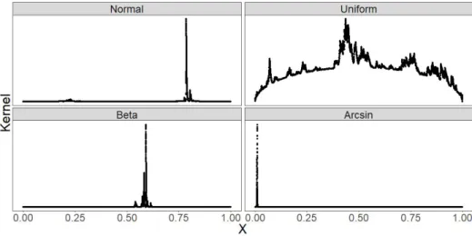
p( ˜ γ| ˜ x)∝ 1 γ1 1 1−γ1 ∗ Γ(Pn i=11(0≤yi< γ1) + 1)Γ(Pni=11(γ1≤yi<1) + 1) Γ(Pn i=11(0≤yi < γ1) +Pni=11(γ1 ≤yi <1) + 2) (1.23)
In order to show a variety of unnormalized posteriors, 50 data points were simulated from each of unif(0,1), N(0,1), beta(2,5), andbeta(0.5,0.5). Figure 1.3 was created by simulating 100,000 points from unif(0,1) and then entering these values into the unnormalized density in Equation
1.23 (refereed to as the ‘Kernel’) using each of these four samples. In the case of the unif(0,1), beta(2,5), andbeta(0.5,0.5) samples, no standardization was applied to the data before calculating the unnormalized posterior density for the cut-point given that the data was already between 0 and 1. TheN(0,1) was standardized, and the effects of the standardization can be seen in the tails of the plot in Figure1.3. Chapter3demonstrates how to use scaling that prevents this from occurring. The exact values of the kernel are not displayed, but the maximum unnormalized density values based on these four samples ranged from 75 to 2X10⁻¹⁰.
Figure 1.3: Unnormalized posterior distribution of γ1 when k = 1 for data from four different distributions with n= 50.