Universal outlier hypothesis testing with applications to anomaly detection

(1)

c

(2)

UNIVERSAL OUTLIER HYPOTHESIS TESTING WITH APPLICATIONS TO ANOMALY DETECTION

BY YUN LI

DISSERTATION

Submitted in partial fulfillment of the requirements

for the degree of Doctor of Philosophy in Electrical and Computer Engineering in the Graduate College of the

University of Illinois at Urbana-Champaign, 2015

Urbana, Illinois Doctoral Committee:

Professor Venugopal V. Veeravalli, Chair Professor Pierre Moulin

Associate Professor Prashant Mehta Assistant Professor Lav R. Varshney

(3)

ABSTRACT

Outlier hypothesis testing is studied in a universal setting. Multiple sequences of observa-tions are collected, a small subset (possibly empty) of which are outliers. A sequence is considered an outlier if the observations in that sequence are distributed according to an “outlier” distribution, distinct from the “typical” distribution governing the observations in the majority of the sequences. The outlier and typical distributions are not fully known, and they can be arbitrarily close. The goal is to design a universal test to best discern the outlier sequence(s). Both fixed sample size and sequential settings are considered in this dissertation. In the fixed sample size setting, for models with exactly one outlier, the gen-eralized likelihood test is shown to be universally exponentially consistent. A single letter characterization of the error exponent achieved by such a test is derived, and it is shown that the test achieves the optimal error exponent asymptotically as the number of sequences goes to infinity. When the null hypothesis with no outlier is included, a modification of the generalized likelihood test is shown to achieve the same error exponent under each non-null hypothesis, and also consistency under the null hypothesis. Then, models with multiple outliers are considered. When the outliers can be distinctly distributed, in order to achieve exponential consistency, it is shown that it is essential that the number of outliers be known at the outset. For the setting with a known number of distinctly distributed outliers, the generalized likelihood test is shown to be universally exponentially consistent. The limiting error exponent achieved by such a test is characterized, and the test is shown to be asymp-totically exponentially consistent. For the setting with an unknown number of identically distributed outliers, a modification of the generalized likelihood test is shown to achieve a positive error exponent under each non-null hypothesis, and consistency under the null hy-pothesis. In the sequential setting, a test with the flavor of the repeated significance test is proposed. The test is shown to be universally consistent, and universally exponentially con-sistent under non-null hypotheses. In addition, with the typical distribution being known, the test is shown to be asymptotically optimal universally when the number of outliers is the largest possible. In all cases, the asymptotic performance of the proposed test when none of the underlying distributions is known is shown to converge to that when only the

(4)

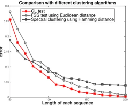
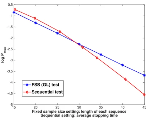
typical distribution is known as the number of sequences goes to infinity. For models with continuous alphabets, a test with the same structure as the generalized likelihood test is proposed, and it is shown to be universally consistent. It is also demonstrated that there is a close connection between universal outlier hypothesis testing and cluster analysis. The per-formance of various proposed tests is evaluated against a synthetic data set, and contrasted with that of two popular clustering methods. Applied to a real data set for spam detection, the sequential test is shown to outperform the fixed sample size test when the lengths of the sequences exceed a certain value. In addition, the performance of the proposed tests is shown to be superior to that of another kernel-based test for large sample sizes.

(5)

To Baba and Mama, who have been there for me since day one. Thank you for everything you have done.

(6)

ACKNOWLEDGMENTS

First and foremost I would like to give special thanks to my advisor Prof. Venugopal Veer-avalli for being a great mentor over the past three years. You are the example that it is not only top-notch research, but also enthusiasm, compassion, and genuine caring for academic advances that make a great scholar. Thank you for providing an encouraging research en-vironment where I had the freedom to pursue various topics and approaches. I could never have made it without your guidance and support, and I am honored to be your student. I also cherish every moment that I shared with you, Starla, and the whole group in GM 3, and I look forward to another round of Pit anytime soon!

I would also like to mention the other members on my doctoral committee, Professors Pierre Moulin, Prashant Mehta, and Lav R. Varshney. Your academic input is greatly appreciated. And your humor made my defense a cheering and enjoyable moment. Thank you.

I would like to express my gratitude to my colleague, Dr. Sirin Nitinawarat. Thank you for your guidance, and your contribution to this work. I admire your humble nature, and your down-to-earth attitude toward research. I am very fortunate to have you as a friend.

A special thanks to my former academic advisor, Prof. Sean P. Meyn. You have been especially helpful in providing academic advices during my first three years as a graduate student. Thank you for being so patient in answering every “silly” question that I had as a fresh graduate.

Last but not least, I would like to thank all the faculty members in the ECE department for giving world-class lectures. I enjoyed every class I took, and I will continue to benefit from what I learnt as a student.

(7)

CHAPTER 1 INTRODUCTION

We consider the following inference problem, which we term outlier hypothesis testing. Among a fixed number of independent and memoryless observation sequences, it is assumed that there is a small subset (possibly empty) of outlier sequences. Specifically, most of the sequences are assumed to be distributed according to a “typical” distribution, while an out-lier sequence is distributed according to an “outout-lier distribution,” distinct from the typical distribution. We are interested in universal settings of this problem, where the outlier and typical distributions are not fully known, and can be arbitrarily close. The goal is to design a test, which does not depend on any unknown distribution, to best identify all the out-lier sequences. Outout-lier hypothesis testing finds possible applications in fraud and anomaly detection in large data sets [1, 2], severe weather prediction, environment monitoring in sensor networks [3], network intrusion and voting irregularity analysis. It also finds appli-cations where the term “outlier” has a positive connotation, such as spectrum sensing and high-frequency trading.

We study both fixed sample size (FSS) and sequential settings of universal outlier hy-pothesis testing. In the FSS setting, the number of observations that are taken before a final decision is made is determined at the outset, and the goal is to identify the outlier sequences with a certain accuracy using as few observations as possible. In the sequential setting, observations are collected sequentially over a period of time. At each time, a test either decides to continue taking one more observation, or to stop and make a final decision. As a result, the number of observations that are collected before the test terminates is not fixed, but rather a random value. The goal in the sequential setting is to achieve a certain accuracy using the fewest observations on average.

1.1

1.2 Dissertation Outline

We now provide a brief overview of each chapter.

• In Chapter 2, we introduce notations, and provide some useful identities and well-known technical facts.

• The FSS setting is studied in Chapter 3, where we show that the GL test is far more efficient for universal outlier hypothesis testing than for the other inference problems, such as homogeneity testing and classification [7–11]. In particular, the GL test is universally exponentially consistent as long as the outlier distributions are distinct from the common typical distribution, and there is indeed an outlier among the sequences. Furthermore, we prove that the GL test is asymptotically efficient in the limit of a large number of sequences in certain settings. When it is also possible that there is no outlier present, a modification of the GL test is shown to be consistent under all hypotheses, and exponentially consistent under every non-null hypothesis.

• In Chapter 4, we generalize our findings in the FSS setting to the sequential setting. We propose a sequential test that has the flavor of the Multihypothesis Sequential Probability Ratio Test [26, 27] and the repeated significance test [28, 29]. The sequen-tial test is shown to be universally consistent, and universally exponensequen-tially consistent

(12)

conditioned on an outlier being present. In addition, when the outliers are identically distributed, it is shown to be asymptotically optimal when the number of outliers is the largest possible, and with the typical distribution being known.

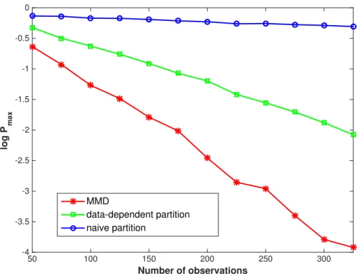
• In Chapter 5, we extend our results to models with continuous alphabets. We pro-pose an FSS test that is of the same spirit as the GL test, and uses non-parametric estimates of the Kullback-Leibler (KL) divergence. The proposed test is shown to be universally consistent for various settings. In addition, we compare the performance of the proposed test with that of a kernel-based test against a synthetic data set. • In Chapter 6, we elaborate on our discussion on the connection between universal

outlier hypothesis testing and cluster analysis. We evaluate the performance of the FSS test and two other clustering algorithms on a synthetic data set, where it is discovered that the FSS test outperforms the clustering algorithms when the sample size is sufficiently large.

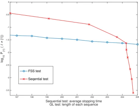
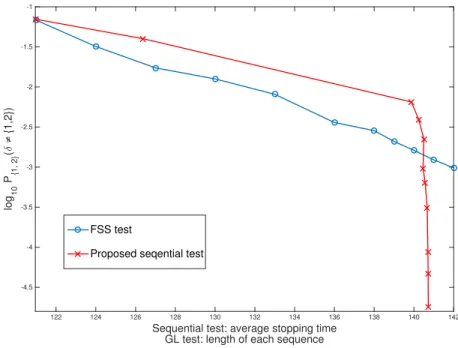
• In Chapter 7, we apply the proposed tests to a real data set for spam detection. The performance of another kernel-based universal test is also evaluated for contrast. The FSS test outperforms three different versions of the kernel-based test for large sample size. And the performance of the sequential test is superior to that of the FSS test when the average stopping time is sufficiently large.

(13)

CHAPTER 2 PRELIMINARIES

Throughout the dissertation, random variables are denoted by capital letters, and their realizations are denoted by the corresponding lower-case letters. All random variables are assumed to take values in finite sets if not specified otherwise, and all logarithms are the natural ones.

For a finite set Y, let Ym _{denote the} _m _{Cartesian product of} _Y_{, and} _P_{(Y) denote the} set of all probability mass functions (pmfs) on Y. The empirical distribution of a sequence

y=ym = (y1, . . . , ym)∈ Ym, denoted by γ =γy ∈ P(Y), is defined as

γ(y) _, 1 m {k = 1, . . . , m:y_k =y} , y∈ Y.

Our results will be stated in terms of various distance metrics between a pair of dis-tribution p, q ∈ P(Y). In particular, we shall consider two symmetric distance metrics: the Bhattacharyya distance and Chernoff information, denoted respectively by B(p, q) and

C(p, q),and defined as (see, e.g., [30])

B(p, q) _, −log X y∈Y p(y)12q(y) 1 2 ! (2.1) and C(p, q) _, max s∈[0,1]−log X y∈Y p(y)sq(y)1−s ! , (2.2)

respectively. Another distance metric, which will be key to our study, is the relative entropy, denoted by D(pkq) and defined as

D(pkq) _, X y∈Y

p(y) log p(y)

(14)

Unlike the Bhattacharyya distance (2.1) and Chernoff information (2.2), the relative entropy in (2.3) is a non-symmetric distance [30].

The following technical facts will be useful; their derivations can be found in [30, Theorem 11.1.2]. Consider random variables Yn _{which are i.i.d. according to} _p_{∈ P(Y). Let} _yn_{∈ Y}n be a sequence with an empirical distribution γ ∈ P(Y). It follows that the probability of such sequenceyn_, _under _p_{and under the i.i.d. assumption, is}

p(yn) = expn−n D(γkp) +H(γ)o, (2.4) where D(γkp) and H(γ) are the relative entropy of γ and p, and entropy ofγ, defined as

D(γkp) _, X y∈Y γ(y) logγ(y) p(y), and H(γ) _, −X y∈Y γ(y) logγ(y),

respectively. Consequently, it holds that for each yn_{, the pmf} _p _{that maximizes} _p₍_yn_{) is}

p=γ, and the associated maximal probability of yn is

γ(yn) = exp−nH(γ) . (2.5)

Next, for each n ≥ 1, the number of all possible empirical distributions from a sequence of length n in Yn _{is upper bounded by (}_n_{+ 1)}|Y|_, _where _|Y| _{denotes the (finite) size of} _Y_. Using this fact, (2.4) and a bound on the size of the set of sequences with the same empirical distribution (see, e.g., [30, Theorem 11.1.3] for details), it can be shown that the probability that the i.i.d. sequence Yn that is distributed according to p has the empirical distribution

γ =q, (for a feasible q) satisfies

P{γ =q} ≤ e−nD(qkp). (2.6) We shall also find the following “sum centroid” inequality and its consequence useful. Con-sider any collection C of distributions on Y :pi, i ∈ C. Then, for any arbitrary distribution

q, X i∈C D pi P j∈Cpj |C| ≤X i∈C D(pikq). (2.7)

(15)

The proof of (2.7) follows from the fact that for any distribution q, X i∈C D pi P j∈Cpj |C| = X i∈C D(pikq)− |C|D P i∈Cpi |C| q .

Now for a pair of distributions p,p¯on Y, particularizing (2.7) to the special case, where C comprises one p distribution andL copies of the ¯pdistribution, and with q in (2.7) being ¯p, we have that D p p+Lp¯ L+ 1 +LD ¯ p p+Lp¯ L+ 1 ≤ D(pkp¯). (2.8)

The proofs in future sections rely on the following lemmas.

Lemma 1. Let Y(1), . . . ,Y(J) be mutually independent random vectors with each Y(j),

j = 1, . . . , J, being n i.i.d. repetitions of a random variable distributed according to pj ∈ P(Y). Let An be the set of all J tuples y(1), . . . ,y(J)

∈ YJ n _{whose empirical distributions} (γ1, . . . , γJ) = γy(1), . . . , γ_y(J)

lie in a closed set E ∈ P(Y)J. Then, it holds that lim n→∞− 1 nlogP n Y(1), . . . ,Y(J)∈An o = min (q1,...,qJ)∈E J X j=1 D(qjkpj). (2.9)

Proof. Let E be the set of all joint distributions in P YJ

with the tuple of their corre-sponding marginal distributions lying inE. It now follows from the closeness ofE inP(Y)J and the compactness of P YJ

that E is also closed in P YJ

. Let An be the set of all

J tuples y(1)_{, . . . ,}_y(J)

= y(1)₁ , . . . , yn(1)

, . . . , y₁(J), . . . , yn(J)

∈ YJ n _{whose joint} empir-ical distribution lies in a closed set E ∈ P YJ

. The lemma then follows by observing that _P n Y(1), . . . ,Y(J)∈ An o = _P n y₁(1), . . . , y(1)n , . . . , y₁(J), . . . , y(nJ) ∈ An o , and by

(16)

invoking Sanov’s theorem to compute the exponent of the latter probability, i.e., lim n→∞− 1 nlogP n Y(1), . . . ,Y(J)∈An o = lim n→∞− 1 nlogP n y₁(1), . . . , y_n(1), . . . , y₁(J), . . . , y_n(J)∈An o = min q∈E D(qkp1× . . . ×pJ) = min (q1,...,qJ)∈E J X j=1 D(qjkpj).

Lemma 2. For any two pmfs p1, p2 ∈ P(Y) with full supports, it holds that

2B(p1, p2) = min q∈ P(Y) D(qkp1) +D(qkp2) . (2.10)

In particular, the minimum on the right side of (2.10) is achieved by

q? = p 1 2 1(y)p 1 2 2(y) P y∈Y p 1 2 1(y)p 1 2 2(y) , y∈ Y. (2.11)

Proof. It follows from the concavity of the logarithm function that

D(qkp1) +D(qkp2) = X y∈Y q(y) log q 2₍_y₎ p1(y)p2(y) =−2X y∈Y q(y) logp 1 2 1(y)p 1 2 2(y) q(y) ≥ −2 log X y∈Y p 1 2 1(y)p 1 2 2(y) (2.12) = 2B(p1, p2).

In particular, equality is achieved in (2.12) by q(y) =q?₍_y_{) in (2.11).}

It is interesting to note that from (2.10), we recover the known inequality discovered in [31]:

(17)

by evaluating the argument distributionqon the right side of (2.10) byp1 andp2,respectively.

Lemma 3. For any two pmfs p1, p2 ∈ P(Y) with full supports, it holds that

C(p1, p2) ≤ 2B(p1, p2).

Proof. The proof follows from an alternative characterization (instead of (2.2)) of theC(p1, p2)

as (cf. [32])

C(p1, p2) = min

q∈P(Y)max (D(qkp1), D(qkp2)), (2.14)

and upon noting that the objective function for the optimization problem in (2.14) is always no larger than that for the one in (2.10).

(18)

CHAPTER 3 FIXED SAMPLE SIZE SETTING

3.1 Exactly One Outlier

ConsiderM ≥3 independent sequences of observations, each of which consists of n indepen-dent and iindepen-dentically distributed (i.i.d.) observations. We denote the k-th observation of the

i-th sequence byY_k(i), which takes values in a finite set denoted byY. It is assumed that only one sequence is the “outlier,” i.e., the observations in that sequence are uniquely distributed (i.i.d.) according to the “outlier” distribution µ ∈ P(Y), while all the other sequences are commonly distributed according to the “typical” distribution π ∈ P(Y). We are interested in a non-parametric setting, in which µ and π are not fully known and can be arbitrarily close. We further assume that bothµandπ have full support over the finite alphabetY. The assumption of µ, π having full support rules out trivial cases where it is straightforward to identify the outlier sequence. Clearly, if M = 2, either sequence can be considered as an outlier; hence, it becomes degenerate to consider outlier hypothesis testing in this case.

It is assumed throughout this section that the outlier distribution is unknown but is independent of the identity of the outlier. In certain applications, it may be natural to consider the model where the outlier distribution can vary depending on the identity of the outlier. This scenario can be viewed as a special case (with the number of outlier sequences being exactly one) of the multiple outlier hypothesis testing problem studied in Section 3.3. Conditioned on the hypothesis that thei-th sequence is the outlier, the joint distribution of all the observations is

pi yM n = pi y(1), . . . ,y(M) = n Y k=1 n µ y_k(i) Y j6=i π y_k(j)o , Li yM n, µ, π , (3.1)

(19)

where y(i) = y₁(i), . . . , y_n(i) , i= 1, . . . , M.

The test for the outlier sequence is done based on a universal rule δ : YM n _{→ {1}_{, . . . , M}_}. In particular, the test δ is not allowed to be a function of (µ, π).

For a universal test, the maximal error probability, which will be a function of the test and (µ, π), is e δ,(µ, π) _, max i=1,...,M X yM n_:_δ₍_yM n₎ ₆₌ _i pi yM n ,

and the corresponding error exponent is defined as

α δ,(µ, π) _, lim n→∞− 1 n loge δ,(µ, π) . (3.2)

Throughout the dissertation, we consider the error exponent as n goes to infinity, while M, and hence the number of hypotheses, is kept fixed. Consequently, the error exponent in (3.2) also coincides with the one for the average probability of error.

A test is termed universally consistent if the maximal error probability converges to zero as the number of samples goes to infinity, i.e.,

e δ,(µ, π) →0, (3.3)

for any (µ, π), µ 6= π as n → ∞. It is termed universally exponentially consistent if the exponent for the maximal error probability is strictly positive, i.e.,

α δ,(µ, π)>0, (3.4)

for any (µ, π),µ6=π.

3.1.1 Generalized Likelihood Test

We now describe the generalized likelihood test in two setups when only π is known, and when neither µ nor π is known, respectively.

For each i= 1, . . . , M, denote the empirical distributions of y(i) _by_γ

i. When π is known and µ is unknown, conditioned on the i-th sequence being the outlier, i = 1, . . . , M, we compute the generalized likelihood ofyM nby replacingµin (3.1) with its maximum likelihood

(20)

(ML) estimate ˆµi ,γi,as ˆ

ptyp_i yM n = Li yM n,µˆi, π

. (3.5)

Similarly, when neither µ nor π is known, we compute the generalized likelihood of yM n

by replacing the µ and π in (3.1) with their ML estimates ˆµi , γi, and ˆπi , P k6=iγk M−1 , i = 1, . . . , M, as ˆ puniv_i yM n = Li yM n,µˆi, πˆi . (3.6)

Finally, we decide upon the sequence corresponding to the largest generalized likelihood to be the outlier. Using (3.5), (3.6), the GL tests in the two cases can be described respectively as

δ yM n = argmax i=1,...,M

ˆ

ptyp_i yM n (3.7)

when onlyπ is known, and

δ yM n = argmax i=1,...,M

ˆ

puniv_i yM n (3.8)

when neither µnor π is known. In (3.7) and (3.8), should there be multiple maximizers, we pick one of them arbitrarily. Using the identity in (2.4), it is straightforward to show that when onlyπ is known, the GL test in (3.7) is equivalent to

δ yM n = argmin i=1,...,M H(γi) + X j6=i [H(γj) +D(γjkπ)] = argmax i=1,...,M D(γikπ), (3.9)

and when neitherπ nor µ is known, the test in (3.8) is equivalent to

δ yM n= argmin i=1,...,M H(γi) + X j6=i h H(γj) +D γj P k6=iγk M−1 i = argmin i=1,...,M X j6=i D γj P k6=iγk M−1 . (3.10)

(21)

3.1.2 Performance of Generalized Likelihood Test

Our first theorem for models with one outlier characterizes the optimal exponent for the maximal error probability when both µand π are known, and when only π is known.

Theorem 1. When µ and π are both known, the optimal exponent for the maximal error probability is equal to

2B(µ, π). (3.11)

Furthermore, the error exponent in (3.11) is achievable by the GL test in (3.7), which uses only the knowledge of π.

Proof. Since we consider the error exponent as n goes to infinity, while M and hence the number of hypotheses is fixed, the ML test, which maximizes the error exponent for the average error probability (averaged over all hypotheses), will also achieve the best error exponent for the maximal error probability. In particular, for any yM n ₌ _y(1)_{, . . . ,}_y(M)

∈ YM n_{, with} _γ

y(i) = γ_i, i = 1, . . . , M, conditioned on the i-th sequence being the outlier,

applying the identity in (2.4), it now follows from (3.1) that the ML test is

δ(yM n) = argmin i=1,...,M

Ui(yM n), where for each i= 1, . . . , M,

Ui(yM n) , D(γikµ) + X

j6=i

D(γjkπ). (3.12)

By the symmetry of the problem, it is clear that _Pi{δ 6=i} is the same for every i = 1, . . . , M; hence,

max

i=1,...,MPi{δ 6=i} = P1{δ6= 1}. It now follows from

P1{δ 6= 1} = P1(∪j6=1{U1 ≥Uj}), (3.13) that P1{U1 ≥U2} ≤ P1{δ6= 1} ≤ M X j=2 P1{U1 ≥Uj}. (3.14)

(22)

Next, we get from (3.12) that

P1{U1 ≥U2} = P1{D(γ1kµ) +D(γ2kπ)

≥D(γ1kπ) +D(γ2kµ)}.

Applying Lemma 1 withJ = 2, p1 =µ, p2 =π, and

E =n(q1, q2) : D(q1kµ) +D(q2kπ)

≥D(q1kπ) +D(q2kµ)

o

,

we get that the exponent for_P1{U1 ≥U2}is given by the value of the following optimization

problem min q1,q2∈ P(Y) D(q1kµ) +D(q2kπ) , (3.15)

where the minimum above is over the set of q1, q2 such that

D(q1kµ) +D(q2kπ) ≥ D(q1kπ) +D(q2kµ).

Note that the objective function in (3.15) is convex in (q1, q2), and the constraint is linear

in (q1, q2). It then follows that the optimization problem in (3.15) is convex. Consequently,

strong duality holds for the optimization problem (3.15) [33]. Then by solving the Lagrangian dual of (3.15), its solution can be easily computed to be 2B(µ, π).

By the symmetry of the problem, the exponents of_P1{U1 ≥Ui}, i6= 1, are the same, i.e.,

for every i= 2, . . . , M,we get lim n→∞−

1

nlogP1{U1 ≥Ui} = 2B(µ, π). (3.16)

From (3.14) and (3.16), using the union bound and that limn→∞ log_nM = 0, we get that lim

n→∞− 1

nlogP1{δ6= 1} = 2B(µ, π). (3.17)

It is now left to prove that when only π is known, the GL test in (3.7) and (3.9) also achieves the optimal error exponent 2B(µ, π).

For each i= 1, . . . , M, denote the test statistic in (3.9) as

(23)

It follows from the same argument leading to (3.17) that lim n→∞− 1 nlogP1{δ 0 _{6= 1}} = lim n→∞− 1 nlogP1 n U₁typ ≤ U₂typ o . (3.18)

The exponent on the right side of (3.18) can be computed by applying Lemma 1 with

J = 2, p1 =µ, p2 =π, and E = (q1, q2) : D(q2kπ)≥D(q1kπ) to be min q1,q2∈P(Y) D(q2kπ)≥ D(q1kπ) D(q1kµ) +D(q2kπ) (3.19)

The optimal value of (3.19) can be computed as follows: min q1,q2∈P(Y) D(q2kπ)≥D(q1kπ) D(q1kµ) +D(q2kπ) (3.20) ≥ min q1 D(q1kµ) +D(q1kπ) (3.21) = 2B(µ, π), (3.22)

where the inequality in (3.21) stems from substituting the constraint in (3.20) into the objective function, and the equality in (3.22) follows from Lemma 2. Since the minimum in (3.21) is achieved by q1 = q? in (2.11) with p1 = µ, p2 = π, and q1 = q2 = q? satisfy the

constraint in (3.20), the inequality in (3.21) is in fact an equality.

Remark 1. It is interesting to note that when only µ is known, one can also achieve the optimal error exponent in (3.11) using a different test that will be presented in Section 3.5. However, we do not yet know if the corresponding version of the GL test, wherein the π in (3.1) is replaced with ˆπi =

P

k6=iγk

M−1 , i= 1, . . . , M, is optimal.

Consequently, in the completely universal setting, when nothing is known about µand π

except that µ6=π, and both µand π have full supports, it holds that for any universal test

δ,

(24)

Given the second assertion in Theorem 1, it might be tempting to think that it would be possible to design a test to achieve the optimal error exponent of 2B(µ, π) universally when neither µnor π is known. Our first example shows that such a goal cannot be fulfilled, and hence we need to be content with a lesser goal.

Example 1: Consider the model with M = 3, and a distinct pair of distributions p6=pon Y with full supports. We now show that there cannot exist a universal test that achieves the optimal error exponent of 2B(µ, π) even just for the two models when µ = p, π = p,

and when µ = p, π = p, both of which have 2B(µ, π) = 2B(p, p). To this end, let us look at the region when a universal test δ decides that the first sequence is the outlier, i.e., A1 = {y3n : δ(y3n) = 1}. Let Pp,p,p denote the distribution corresponding to the first

hypothesis of the first model, i.e., when y(1) _{are i.i.d. according to} _p, _and _y(2) _and _y(3) _are

i.i.d. according top. Similarly, let_Pp,p,p denote the distribution corresponding to the second hypothesis of the second model, i.e., when y(2) _{are i.i.d. according to} _p, _and _y(1) _and _y(3)

are i.i.d. according top.Suppose thatδ achieves the best error exponent of 2B(p, p) for the first model when µ=p, π =p. Then, it must hold that

lim n→∞ − 1 n logPp,p,p{A c 1} ≥ 2B(p, p). (3.24)

It now follows from (3.24) and the classic result of Hoeffding [6] in binary hypothesis testing (see, e.g., [34][Exercise 2.13 (b)]) that

lim n→∞ − 1 nlogPp,p,p{A1} ≤h min q(y1,y2,y3) D(q(y1)kp) +D(q(y2)kp) +D(q(y3)kp) i+ ≤h min q(y1,y2,y3) 2B(p, p) +D(q(y3)kp) −D(q(y3)kp) i+ ≤ 2B(p, p)−D(pkp)+ = 0, (3.25) where each minimum on the right side above is taken over the set ofq(y1, y2, y3) such that

D(q(y1)kp) +D(q(y2)kp) +D(q(y3)kp)≤2B(p, p).

The last equality in (3.25) follows from Lemma 2 in Chapter 2. Consequently, the test cannot yield even a positive error exponent for the second model when µ=p, π =p.

(25)

Remark 2. It is interesting to contrast this example for outlier hypothesis testing with the results (Theorems 2 and 3 in [35]) for universal coding over discrete memoryless channels (DMCs). Specifically, Theorems 2 and 3 in [35] establish that the optimal error exponent at zero rate is universally achieved for all DMCs, whereas the optimal error exponent 2B(µ, π) for outlier hypothesis testing here cannot be universally achieved. The difference between these two results stems from the following distinctions between the nature of these two problems. First, in universal coding, the encoder and decoder are jointly optimized to achieve universality. On the other hand, in outlier hypothesis testing, when properly interpreted, only the decoding is allowed to be optimized, while the encoding scheme is fixed by the structure of the distributions of observations among all hypotheses, and cannot be chosen. Second, the zero-rate error exponent in [35] applies only for the case when the number of messages grows to infinity with the blocklength sub-exponentially. In contrast, the number of hypotheses in outlier hypothesis testing is fixed and does not grow with the number of observations in each sequence.

To summarize, the results in [35] cannot be applied to our problem. Had the results in [35] been applicable, Theorems 2 and 3 in [35] would have implied that the optimal error exponent 2B(µ, π) is achieved universally for outlier hypothesis testing as well. However, Example 1 proves otherwise.

Example 1 shows explicitly that when neitherµnorπis known, it is impossible to construct a test that achieves 2B(µ, π) universally. In fact, the example shows that had we insisted on achieving the best error exponent of 2B(µ, π) for some pairs of µ, π, it might not be possible to achieve evenpositive error exponents for some other pairs ofµ, π. This motivates us to seek instead a test that yields just a positive (no matter how small) error exponent

α(δ,(µ, π)) > 0 for every µ, π, µ 6= π, i.e., achieving universally exponential consistency. One of our main contributions in this chapter is to show that GL tests are indeeduniversally exponentially consistent under various settings, including the current single outlier setting for every fixed M.

Theorem 2. The GL test δ in (3.8) is universally exponentially consistent. Furthermore, for every pair of distributions µ, π, µ 6=π, it holds that

α δ,(µ, π)

= min q1,...,qM

D(q1kµ) +D(q2kπ)

(26)

where the minimum above is over the set of (q1, . . . , qM) such that X j6=1 D qj P k6=1qk M−1 ≥X j6=2 D qj P k6=2qk M−1 . (3.27)

Proof. For each i= 1, . . . , M, denote the test statistic in (3.10) as

U_iuniv _,X j6=i D γj P k6=iγk M−1 . (3.28)

The same argument leading to (3.17) yields that lim n→∞− 1 nlogP1{δ6= 1} = lim n→∞− 1 nlogP1 n U₁univ ≥ U₂univo. (3.29) By applying Lemma 1 withJ =M, p1 =µ, pj =π, j= 2, . . . , M, and

E = (q1, . . . , qM) : X j6=1 Dqj P k6=1qk M−1 ≥ X j6=2 D qj P k6=2qk M−1 , (3.30)

the exponent on the right side of (3.29) can be computed to be min

(q1,...,qM)∈E

D(q1kµ) +D(q2kπ) +. . .+D(qMkπ). (3.31) Unlike the convex optimization problems in (3.15) and (3.19), the optimization problem in (3.31) for the completely universal setting is much more complicated, and a closed-form solution is not available. However, we show that the value of (3.31) is strictly positive for every µ6=π. In particular, it is not hard to see that the objective function is continuous in

q1, . . . , qM and the constraint setE is compact. Therefore the minimum in (3.31) is achieved by some (q?₁, . . . , q?_M)∈E. Note that the objective function in (3.31) is always non-negative. In order for the objective function in (3.31) to be zero, the minimizing (q?

1, . . . , q?M) has to satisfy that q?

1 = µ, qi? = π, i = 2, . . . , M. Since this collection of distributions is not in the constraint set E in (3.30), we get that the optimal value of (3.31) is strictly positive for every µ6=π.

(27)

that the random empirical distributions (γ1, . . . , γM) satisfy lim n→∞Pi n 1 M PM j=1γj− 1 Mµ+ M−1 M π 1 > o = 0, (3.32)

where k · k1 denotes the 1-norm of the argument distribution. Since _M1 µ+ M_M−1π → π as

M → ∞, heuristically speaking, a consistent estimate of the typical distribution can readily be obtained asymptotically in M from the entire observations before deciding upon which sequence is the outlier. This observation and the second assertion of Theorem 1 motivate our study of the asymptotic performance (achievable error exponent) of the GL test in (3.8) when M → ∞(after having taken the limit as n goes to infinity first).

Our last result for models with one outlier shows that for the completely universal setting, the GL test in (3.8) isasymptotically efficient, i.e., as M → ∞, it achieves the optimal error exponent in (3.11) corresponding to the case in which both µ and π are known.

Theorem 3. For each M ≥3, the exponent for the maximal error probability achievable by the GL test δ in (3.8) is lower bounded by

min q∈ P(Y) D(qkπ)≤_M1₋₁ 2B(µ,π)+Cπ 2B(µ , q), (3.33) where Cπ ,−log min y∈Y π(y)

<∞ by the fact that π has a full support.

The lower bound for the error exponent in (3.33) is nondecreasing inM ≥3. Furthermore, asM → ∞, this lower bound converges to the optimal error exponent2B(µ, π); hence, the GL testδ in (3.8) achieves the optimal error exponent asymptotically as the number of sequences approaches infinity, i.e.,

lim

M→∞α δ,(µ, π)

= 2B(µ, π), (3.34)

which from Theorem 1 is equal to the optimal error exponent when both µand π are known. Proof. By the continuity of the objective function on the right side of (3.26) and the com-pactness of the constraint set (3.27), for each M ≥ 3, the optimal value on the right side of (3.26), denoted by V?_{, is achieved by some (}_q?

1, . . . , qM? ). It then follows from (3.26) and (3.27) that

(28)

V? ≥D(q₁?kµ) +X j6=1 D q?_jkπ −X j6=1 Dq_j? P k6=1q?k M−1 +X j6=2 Dq_j? P k6=2q?k M−1 = D(q₁?kµ) +X j6=2 Dq_j? P k6=2q?k M−1 +X j6=1 X y∈Y q_j?(y) log 1 M−1 P k6=1q ? k(y) π = D(q₁?kµ) +X j6=2 D q_j? P k6=2q?k M−1 + (M −1)D P k6=1qk? M−1 π ≥ D(q?₁kµ) +Dq₁? P k6=2qk? M−1 ≥ 2Bµ , P k6=2q?k M−1 = 2Bµ , q?1 M−1 + M−2 M−1 PM k=3q?k M−2 , (3.35)

where the last inequality follows Lemma 2.

On the other hand, it follows from (3.23) that the value on the right side of (3.26), V?, satisfies 2B(µ, π) ≥ V? = D(q₁?kµ) +X j6=1 D q?_j kπ ≥ M X j=3 D q?_jkπ ≥ (M−2)D_M1₋₂PM_k₌₃q?_k π , (3.36)

where the last inequality follows from the convexity of relative entropy.

Combining (3.35) and (3.36), we get that the valueV? on the right side of (3.26) is lower bounded by min q1,q∈ P(Y) (M−2)D(qkπ)≤2B(µ,π) 2Bµ , _M1₋₁q1+ M_M−−21q . (3.37)

(29)

Note that the constraint in (3.37) can be equally written as

D(q1kπ) + (M −2)D(qkπ) ≤ 2B(µ, π) +D(q1kπ).

Also by the convexity of relative entropy, it follows that

D(q1kπ) +(M −2)D(qkπ) ≥ (M −1)D q1+(M−2)q M−1 π .

As a result, the optimal value of (3.37) is further lower bounded by the optimal value of min q1,q∈ P(Y) (M−1)D(_M1₋₁q1+M_M−₋2₁qkπ) ≤ 2B(µ,π)+D(q1kπ) 2Bµ , _M1₋₁q1+ M_M−₋2₁q . (3.38)

By the fact thatπ has full support, it holds that

D(q1kπ) ≤ −log min y∈Y π(y) = Cπ ≤ ∞. (3.39)

Proceeding from (3.38), by using (3.39), we get that the optimal value of (3.26) is lower bounded by min q0_{∈ P}₍_Y₎ D(q0_k_π₎_≤ 1 M−1(2B(µ,π)+Cπ) 2B(µ , q0). (3.40)

For anyµ, π ∈ P(Y) with full supports, it holds that lim M→∞ 1 M −1 2B(µ, π) +Cπ = 0.

This and the continuity ofD(qkπ) inq(πhas a full support) establish (3.34): the asymptotic optimality of the GL test in the regime of large number of sequences.

Furthermore, for any µ, π ∈ P(Y), µ6= π, the value of _M1₋₁(2B(µ, π) +C(π)) is strictly decreasing with M. Consequently, the feasible set in (3.33) is nonincreasing with M, and hence the optimal value of (3.33) is nondecreasing withM.

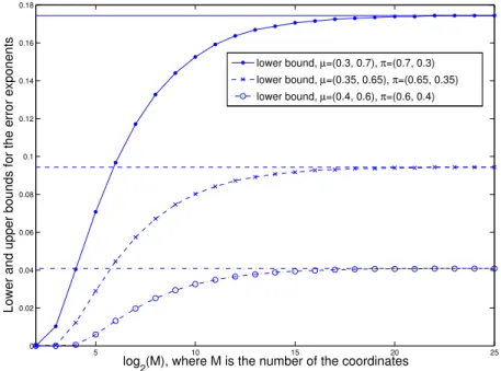
Example 2: We now provide some numerical results for an example with Y = {0,1}. Specifically, the three plots in Figure 3.1 are for three pairs of outlier and typical distributions being µ = (p(0) = 0.3, p(1) = 0.7), π = (0.7,0.3); µ = (0.35,0.65), π = (0.65,0.35); and

(30)

µ= (0.4,0.6), π= (0.6,0.4),respectively. Each horizontal line corresponds to 2B(µ, π), and each curve line corresponds to the lower bound in (3.33) for the error exponent achievable by the GL test in (3.8). As shown in these plots, the lower bounds converge to 2B(µ, π) as

M → ∞, i.e., the GL test in (3.8) is asymptotically optimal for all three pairs of µ, π, and, indeed, for all µ6=π.

5 10 15 20 25 0 0.02 0.04 0.06 0.08 0.1 0.12 0.14 0.16 0.18 log

2(M), where M is the number of the coordinates

Lower and upper bounds for the error exponents

lower bound, µ=(0.3, 0.7), π=(0.7, 0.3) lower bound, µ=(0.35, 0.65), π=(0.65, 0.35) lower bound, µ=(0.4, 0.6), π=(0.6, 0.4)

Figure 3.1: Lower and upper bounds for the achievable error exponent of the GL test

3.2 At Most One Outlier Sequence

A natural question that arises at this point is what would happen if it is also possible that no outlier is present. To answer this question, we now consider models that append an additional nullhypothesis with no outlier to the previous models consider in Section 3.1. In particular, under the null hypothesis, the joint distribution of all the observations is given by p0 yM n = n Y k=1 M Y i=1 π y(_ki).

A universal test δ : YM n _{→ {0}_,₁_{, . . . , M}_} _{will now also accommodate for an additional} decision for the null hypothesis. Correspondingly, the maximal error probability is now

(31)

computed with the inclusion of the null hypothesis according to e δ,(µ, π) _, max i=0,1,...,M X yM n_:_δ₍_yM n₎ ₆₌ _i pi yM n .

With just one additional null hypothesis, contrary to the previous models with one outlier, it becomes impossible to achieve universally exponential consistencyeven with the knowledge of the typical distribution.

Proposition 4. For the setting with the additional null hypothesis, there cannot exist a universally exponentially consistent test even when the typical distribution is known.

Proof. The proposition follows as a special case of the second assertion of Theorem 10, the proof of which is deferred to Section 3.4

In typical applications such as environment monitoring and fraud detection, the conse-quence of a missed detection of the outlier can be much more catastrophic than that of a false positive. In addition, Proposition 4 tells us that there cannot exist a universal test that yields exponential decays for both the conditional probability of false positive (under the null hypothesis) and the conditional probabilities of missed detection (under all non-null hy-potheses). Consequently, it is natural to look for a universal test fulfilling a lesser objective: attaining universally exponential consistency for conditional error probabilities under all the non-nullhypotheses, while seekingonly universal consistency for the conditional error prob-ability under the null hypothesis. We now show that such a test can be obtained by slightly modifying the GL test in (3.8). Furthermore, in addition to achieving universal consistency under the null hypothesis, this new test achieves the same exponent as in (3.26), (3.27) in Theorem 2 for the conditional error probabilities under allnon-null hypotheses.

3.2.1 Proposed Universal Test

We modify the previous test in (3.8) to allow for the possibility of deciding for the null hypothesis as follows: δ(yM n) =        arg max i=1,...,M ˆ puniv i (yM n), if max j6=k 1 n log ˆp univ j (yM n) −log ˆpuniv_k (yM n)> λn, 0, otherwise, (3.41)

where λn = Θ(log_nn) and the ties in the first case of (3.41) are broken arbitrarily. Using the identity in (2.4), it is straightforward to show that test in (3.41) can be equivalently written

(32)

as δ(yM n) =              arg min i=1,...,M P k6=i Dγk P l6=iγl M−1 , if max j6=j0 P k6=j Dγk P l6=jγl M−1 − P k6=j0 Dγk P l6=j0γl M−1 > λn, 0, otherwise. (3.42)

3.2.2 Performance of Proposed Test

Theorem 5. For every pair of distributions µ, π, µ 6= π, the test in (3.41) yields a pos-itive exponent for the conditional probability of error under every non-null hypothesis i = 1, . . . , M, and a vanishing conditional probability of error under the null hypothesis. In par-ticular, the achievable error exponent under every non-null hypothesis is the same as that given in (3.26), (3.27), i.e., for each i= 1, . . . , M, the test in (3.41) achieves

lim n→∞− 1 n log (Pi{δ 6=i}) = min q1,...,qM D(q1kµ) +D(q2kπ) +. . .+D(qMkπ), (3.43) where the minimum above is over the set of (q1, . . . , qM) satisfying (3.27). In addition, the test also yields that

lim

n→∞P0{δ 6= 0} = 0. (3.44)

Proof. We start by establishing universal consistency of the test under the null hypothesis. Applying the identity in (2.4) to the test statistics in (3.41), it holds that

P0{δ6= 0} ≤ P0 ∪M j=1{Ujuniv ≥λn} ≤ M X j=1 P0 U_juniv ≥λn = M_P0 U₁univ ≥λn , (3.45)

where U_juniv is defined in (3.28), and the last equality follows from the fact that all y(i),

(33)

We now proceed to bound _P0{U1univ ≥λn} as follows: P0{U1univ ≥λn} =_P0 X j6=1 Dγj P k6=1γk M−1 ≥λn =_P0 X j6=1 D(γjkπ)−(M−1)D P k6=1γk M−1 π ≥λn ≤_P0 X j6=1 D(γjkπ)≥λn ≤_P0 ∪j6=1 D(γjkπ)≥ 1 M−1λn ≤(M −1)_P0 n D(γ2kπ)≥ 1 M −1λn o , (3.46)

where the first inequality follows from the non-negativity of the relative entropy, and the last inequality follows from the fact that ally(j)_,_j _{6= 1, are identically distributed according}

to π. By the fact that the set of all possible empirical distributions of (y1, . . . , yn) is upper bounded by (n+ 1)|Y| (cf. [30][Theorem 11.1.1]), and (2.4), we get that

P0 n D(γ2kπ)≥ 1 M−1λn o ≤ (n+ 1)|Y|exp(− n M −1λn). (3.47)

It then follows from (3.45), (3.46) and (3.47) that P0{δ 6= 0} ≤M2exp n − n M−1λn+|Y|log(n+ 1) o . (3.48) By choosing λn = 2(M −1)|Y| log (n+1)

n ,we get from (3.48) that lim

n→∞P0{δ 6= 0} = 0.

Next we treat the exponent for the conditional probability of error under every non-null hypothesis. In particular, by the symmetry of the test (3.41) among all the M non-null hypotheses, it suffices to consider the conditional error probability under just the first

(34)

hypothesis, which can be upper bounded as follows: P1{δ 6= 1} ≤ P1 ∪j6=1 n U₁univ ≥ U_juniv−λn o ≤ X j6=1 P1 n U₁univ ≥ U_juniv−λn o ≤ (M−1)_P1 n U₁univ ≥ U₂univ−λn o . (3.49)

For an arbitraryλ0 >0, asλn →0,it holds thatλn ≤λ0 forn sufficiently large and hence

that P1 n U₁univ ≥U₂univ−λn o ≤ _P1 n U₁univ ≥ U₂univ−λ0 o . (3.50)

The exponent of the right side of (3.50) can be computed by applying Lemma 1 withJ =M,

p1 =µ, pj =π, j = 2, . . . , M and (cf.(3.28)) E(λ0) , (q1, . . . , qM) : X j6=1 Dqj P k6=1qk M−1 ≥ X j6=2 Dqj P k6=2qk M−1 −λ0 to be min (q1,...,qM)∈E(λ0) D(q1kµ) +D(q2kπ) +. . .+D(qMkπ). (3.51) Since λ0 can be arbitrarily close to zero, the exponent for the left side of (3.50) is lower

bounded by lim λ0→0 min (q1,...,qM)∈E(λ0) D(q1kµ) +D(q2kπ) +. . .+D(qMkπ). Let E _, (q1, . . . , qM) : X j6=1 Dqj P k6=1qk M−1 ≥ X j6=2 D qj P k6=2qk M−1 .

(35)

in (3.51) is continous, the exponent for the left side of (3.50) is lower bounded by min

(q1,...,qM)∈E

D(q1kµ) +D(q2kπ) +. . .+D(qMkπ), (3.52) as required.

Since under every non-null hypothesis, the modified test in (3.41) achieves the same ex-ponent (the value of the optimization problem in (3.26) and (3.27)) for the conditional error probability as the GL test in (3.8) when the null hypothesis is absent, we get the following corollary by just observing that Theorem 3 was proved by finding a suitable lower bound for the value of the optimization problem in (3.26) and (3.27).

Corollary 6. For each M ≥ 3 and under every non-null hypothesis i = 1, . . . , M, the exponent for the conditional error probability achievable by the test in (3.41) is lower bounded as

lim n→∞−

1

n log (Pi{δ 6=i})≥q∈ Pmin(Y)2B(µ , q), (3.53)

where the minimum above is over the set of q such that

D(qkπ) ≤ 1 M −1 2B(µ, π) +Cπ , and Cπ ,−log min y∈Y π(y)

<∞. Consequently, as M → ∞, this lower bound converges to the optimal error exponent 2B(µ, π), i.e., for every i= 1, . . . , M, the test in (3.41) achieves

lim

M→∞ nlim→∞− 1

n log (Pi{δ 6=i}) = 2B(µ, π),

while also yielding that

lim

n→∞P0{δ 6= 0} = 0.

3.3 Multiple Distinctly Distributed Outliers

We now generalize our results in the previous sections to models with multiple outlier se-quences. With more than one outlier sequence, it may be more natural to consider models for which the different outlier sequences are distinctly distributed, and therefore our models will allow for this possibility.

(36)

We start by describing a generic model with possibly distinctly distributed outliers, the number of which is not known exactly. Specifically, it is assumed that there are up to

K ≥ 1 outliers. Note that the current model with K = 1 corresponds to the single outlier setting where the outlier distribution can vary according to the index of the out-lier sequence. As in Section 3.1, we denote the k-th observation of the i-th sequence by

Y_k(i) ∈ Y, i = 1, . . . , M, k = 1, . . . , n. Most of the sequences are commonly distributed ac-cording to the “typical” distribution π ∈ P(Y) except for a small (possibly empty) subset

S ⊂ {1, . . . , M}of “outlier” sequences, each of which is assumed to be distributed according to an outlier distribution µi, i∈ S. Nothing is known about {µi}M_i₌₁ and π except that each

µi 6=π, i= 1, . . . , M, and that allµi, i= 1, . . . , M, and π have full supports. In the follow-ing presentation, we sometimes consider the special case when all the outlier sequences are identically distributed, i.e., µi =µ,i= 1, . . . , M.

For the hypothesis corresponding to an outlier subsetS ⊂ {1, . . . , M}, |S|< M₂, the joint distribution of all the observations is given by

pS yM n = pS y(1), . . . ,y(M) = n Y k=1    Y i∈S µi y_k(i) Y j /∈S πy_k(j)    , (3.54) where y(i) =y₁(i), . . . , y(_ni), i= 1, . . . , M.

We refer to the unique hypothesis corresponding to the case with no outlier, i.e., S =∅, as the null hypothesis. In the following subsections, we shall consider different settings, each being described by a suitable set S comprising all possible outlier subsets.

The test for the outlier subset is done based on a universal rule δ : YM n _{→ S. In} particular, the test δ is not allowed to be a function of {µi}

M i=1, π

.

For a universal test, the maximal error probability, which will be a function of the test and {µi}M_i₌₁, π , is eδ,{µi} M i=1, π , max S∈S X yM n_:_δ₍_yM n₎ ₆₌_S pS yM n , (3.55)

(37)

and the corresponding error exponent is defined as αδ,{µi}M_i₌₁, π , lim n→∞− 1 nlog e δ,{µi}M_i₌₁, π .

A universal testδis termeduniversally exponentially consistentif for everyµi, i= 1, . . . , M, µi 6=

π, it holds that α δ, {µi}M_i₌₁, π >0.

3.3.1 Necessary Condition for Existence of Universally Exponentially

Consistent Test

Our first result concerns the necessary condition for the existence of a universally exponen-tially consistent test when the outliers can be distinctly distributed in an arbitrary manner. In our model for this section, the assumption of a known number of outliers is in fact critical, as a lack thereof would make it impossible to construct a universally exponentially consistent test even when there are always some outliers.

Theorem 7. When the outliers can be distinctly distributed, with the number of outliers being unknown, there cannot exist a universally exponentially consistent test, even when the typical distribution is known and when the null hypothesis is excluded, i.e., there is at least one outlier regardless of the hypothesis.

Proof. Without loss of generality, we can consider the following two hypotheses. The first hypothesis has S1 as the set of outliers, and the second hypothesis hasS2,whereS1 ⊂S2. It

suffices to prove that even when π and {µi}i∈S1 are known, there cannot exist a universally

exponentially consistent test in differentiating such two hypotheses.

For any test δ : YM n _{→ {1}_,_{2}, let} _δ _{= 1 denote a decision in favor of the hypothesis} with S1 being the outliers, and 2 the hypothesis with S2. We first show that in order to

distinguish betweenS1 and S2, the empirical distributions of all the sequencesγ1, . . . , γM,π and {µi}i∈S1 are sufficient statistics for the error exponent. In particular, we now show that

given any test, there is another test that achieves the same error exponent with its decision being made basedonly onthe empirical distributions of all M sequences,π and {µi}i∈S1. To

this end, for feasible empirical distributions (for certain n) γ1, . . . , γM,let us denote the set of all M sequences conforming to these empirical distributions by T(γ1,...,γM). Among these

observation sequences, let us denote the set of M sequences for which δ decides for S1 by

T₍1_γ,π

1,...,γM),which may depend on π and{µi}i∈S1. Now consider another test δ

0 _{which decides} on one of the two hypotheses based only onγ1, . . . , γM,πand {µi}i∈S1. Specifically, this new

(38)

test is such that for all M sequences with empirical distributions γ1, . . . , γM, it decides for

S1 if |T₍1_γ,π₁_,...,γ_M₎| ≥ ₂1|T(γ1,...,γM)|, and for S2 otherwise. It follows from this construction of δ

0 that for any {µi}Mi=1 and π,

max (_PS1{δ 0 ₆₌ S1},PS2{δ 0 ₆₌ S2}) ≤ 2 max (_PS1{δ6=S1},PS2{δ6=S2}),

where _PS₁ and _PS₂ are the distributions under the hypothesis with S1 and S2 being the set

of outliers, respectively. Consequently, the error exponent achievable by δ0 is the same as that achievable by δ for any {µi}Mi=1 and π, where µi 6=π, i= 1, . . . , M.

We now consider tests that only depend on the empirical distributions of all the sequences

γ1, . . . , .γM, π and {µi}Mi=1. Let assume that for any fixed π and {µi}i∈S1, there exists

= (π,{µi}i∈S1) > 0 such that

lim n→∞−

1

nlogP1{δ6= 1} > , (3.56)

where _P1 is the distribution under the hypothesis withS1 being the outliers. It now follows

from (3.56) and Lemma 1 that the set A of all M tuples y(1)_{, . . . ,}_y(M)

∈ YM n _whose empirical distributions (γ1, . . . , γM) lie in the following set

E _,n(q1, . . . , qM) : X i∈S1 D(qikµi) + X j /∈S1 D(qikπ)≤ 2 o (3.57)

must be such that

A⊆ {δ = 1}. (3.58)

By applying Lemma 1 again, but now with respect to the hypothesis with S2 being the

outliers, we get that lim n→∞− 1 nlogP2{δ6= 2} ≤ min (q1,...,qM)∈E X i∈S1 D(qikµi) + X j∈S2\S1 D(qjkµj) + X k /∈S2 D(qkkπ), (3.59)

where _P2 is the distribution under the hypothesis with S2 being the outliers. Since is

independent of {µj}j∈S2\S1, we can pick {µj}j∈S2\S1 to be such that

P j∈S2\S1

(39)

now follows from the definition of E, (3.59) and Lemma 1 that lim

n→∞− 1

nlogP2{δ6= 2} = 0,

which establishes the assertion.

Remark 3. The negative result in Theorem 7 should not be considered as overly pessimistic. It should be viewed as a theoretical result that holds only when each of the outliers can be arbitrarily distributed. In practice, there will likely be modeling constraints that would confine the set of all possible tuples of the distributions of all outliers. An extreme case of such constraints is when all the outliers are forced to be identically distributed, which is when universally exponential consistency is indeed attained (cf. Theorem 10) if the null hypothesis is excluded. An interesting future research direction would be to characterize the “least” stringent joint constraint on the distributions of the outliers that still allows us to construct universally exponentially consistent tests.

For the rest of this section, we restrict our attention to the case in which the number of outliers, denoted by K ≥ 1, is known at the outset, i.e., |S| =K, for every S ∈ S. Unlike the models in Sections 3.1 and 3.2 where the outlier sequence is always distributed according to a fixed distribution µ 6= π regardless of its identity i = 1, . . . , M, in our model for this section, the distributions of different outlier sequences µi, i∈S,can vary across the indices of the sequences, i∈S.

To contrast with the universal setting, the next result characterizes the optimal error exponent for the maximal error probability when both µ and π are known.

Proposition 8. For every fixed number of outliers K ≥ 1, when all the µi, i = 1, . . . , M, and π are known, the optimal error exponent is equal to

min

1≤i<j≤M C(µi(y)π(y 0

), π(y)µj(y0)). (3.60) When all outlier sequences are identically distributed, i.e., µi =µ6=π, i= 1, . . . , M, this optimal error exponent is independent of M and is equal to

2B(µ, π). (3.61)

Proof. The proposition follows from a well-known result in detection and estimation in the context of the multihypothesis testing problem[36]. In particular, the optimal error exponent for testing M hypotheses with i.i.d. observations with respect top1, p2, . . . , pM is character-ized as min

(40)

When all the {µi}M_i₌₁ and π are known, the underlying outlier hypothesis testing prob-lem is just a multihypothesis testing probprob-lem based on i.i.d. vector observations (with M

independent components) and consequently, the optimal error exponent can be computed as min S6=S0C Y i∈S µi(yi) Y j /∈S π(yj), Y i∈S0 µi(yi) Y j /∈S0 π(yj) = min S6=S0C _Y i∈S\S0 µi(yi) Y j∈S0_\_S π(yj), Y i∈S\S0 π(yi) Y j∈S0_\_S µj(yj) = min S6=S0_smax_∈_[0_,_1]−log " X yi, i∈S\S0 yj, j∈S0\S Y i∈S\S0 µi(yi) 1−s π(yi) s Y j∈S0_\_S π(yj) 1−s µj(yj) s # (3.62) = min

1≤i<j≤M smax∈[0,1] −log

" X yi,yj µi(yi)1 −s π(yi)sπ(yj)1 −s µj(yj)s # (3.63) = min 1≤i<j≤M C(µi(y)π(y 0 ), π(y)µj(y0)),

where the equality in (3.63) follows by virtue of fact that the outer minimum in (3.62) is attained among the pairs ofS, S0,with the largest number of sequences in their intersections:

K−1.

When all the outliers are identically distributed, i.e., µi = µ, i = 1, . . . , M, this optimal error exponent can be further simplified to be

min

1≤i<j≤M C(µi(y)π(y 0

), π(y)µj(y0))

= C(µ(y)π(y0), π(y)µ(y0)) = 2B(µ, π). (3.64)

3.3.2 Generalized Likelihood Test

We now give a summary of the GL test for the current models with a known number of outliers for both the setting when only π is known and for the completely universal setting. Conditioned on the outlier subset being S ∈ S, the likelihood ofyM n _{is a function of the} outlier indices, and the typical and outlier distributions (cf. (3.54)), i.e.,

pS yM n

= L yM n,{µi}i∈S, π

. (3.65)

(41)

(3.65) with its ML estimate ˆµi ,γi, i∈S, as ˆ

ptyp_S yM n = L yM n,{µˆi}i∈S, π

. (3.66)

Similarly, for the completely universal setting, we compute the generalized likelihood of

yM n by replacing the µi and π in (3.65) with their ML estimates ˆµi , γi, i ∈ S, and ˆ πS , P k /∈Sγk M−K , as ˆ p_Suniv yM n = L yM n,{µˆi}i∈S, ˆπS . (3.67)

The test then selects the hypothesis under which the generalized likelihood is maximized (ties are broken arbitrarily), i.e.,

δ yM n = argmax S⊂{1,...,M}, |S|=K

ˆ

ptyp_S (3.68)

for the setting when only π is known, and

δ yM n

= argmax

S⊂{1,...,M}, |S|=K ˆ

puniv_S (3.69)

for the completely universal setting, respectively. It is straightforward to show using (2.4) that when onlyπ is known, the GL test in (3.68) is equivalent to

δ yM n = argmin S⊂{1,...,M}, |S|=K

X

j /∈S

D(γjkπ), (3.70)

and when neitherπ nor {µi}M_i₌₁ is known, the test in (3.69) is equivalent to

δ yM n = argmin S⊂{1,...,M}, |S|=K X j /∈S D γj P k /∈Sγk M−K . (3.71)

3.3.3 Performance of Generalized Likelihood Test

Theorem 9. For every fixed number of outliers K ≥1, when only π is known but none of

µi, i= 1, . . . , M is known, the error exponent achievable by the GL test in (3.66) is equal to min

(42)

When all outlier sequences are identically distributed, i.e., µi = µ, i = 1, . . . , M, this achievable error exponent is equal to

2B(µ, π), (3.73)

which, from Proposition 8, is the optimal error exponent when µ is also known. Proof. For each S ⊂ S, denote the test statistic in (3.70) as

U_Styp _,X

j /∈S

D(γjkπ). (3.74)

Consider the test δ in (3.68) and (3.70). It follows from the fact that for every S ∈ S,

PS{δ6=S} = PS ∪ S0₆₌_S U_Styp ≥U_Styp0 that max S6=S0 PS n U_Styp ≥U_Styp0 o ≤max S∈S PS{δ 6=S} ≤max S∈S X S0₆₌_S PSUStyp ≥U typ S0 ≤(|S| −1) max S6=S0PS U_Styp ≥U_Styp0 . (3.75)

Next, we get from (3.74) that for any S 6=S0 ∈ S,

PSUStyp ≥U typ S0 =PS ( X i /∈S D(γikπ)≥ X i /∈S0 D(γikπ) ) .

Applying Lemma 1 withJ =M, pi =µi, i∈S, pj =π, j /∈S,and

E = ( (q1, . . . , qM) : X i /∈S D(qikπ)≥ X i /∈S0 D(qikπ) ) , (3.76)

we get that the exponent for _PS

(43)

optimization problem: min {qi}i∈S\S0,{qj}j∈S0\S X i∈S\S0 D(qikµi) + X j∈S0_\_S D(qjkπ), (3.77)

where the minimum above is over the set of {qi}_i∈S\S0, {qj}_j_∈_S0_\_S, such that

X j∈S0_\_S D(qjkπ) ≥ X i∈S\S0 D(qikπ).

We now show that the optimum value in (3.77) is equal to P i∈S\S0

2B(µi, π). First, we show that the latter is a lower bound for the former. Substituting the constraint in (3.77) into the objective function, we get that the value of (3.77) is lower bounded by

min {qi}i∈S\S0 X i∈S\S0 D(qikµi) +D(qikπ) = X i∈S\S0 2B(µi, π), (3.78)

where the equality follows from Lemma 2. Second, note that |S\S0| is always equal to |S0\S|, and, hence, we can make a suitable correspondence between elements of S\S0 to those of S0\S. The converse implication now follows by assigning for every i ∈ S\S0, and the corresponding j ∈ S0\S, qi = qj = µi(y)

1/2_π₍_y₎1/2

P

y0∈Y

µi(y0)1/2π(y0)1/2

, and note that this assignment trivially satisfies the constraint in (3.77) and gives rise to the objective function being equal to P

i∈S\S0

2B(qi, π).

Lastly, it follows from (3.75) that lim n→∞− 1 nlog max S∈S PS{δ6=S} = min S6=S0 X i∈S\S0 2B(µi, π) = min 1≤i≤M 2B(µi, π). When µi =µ,i= 1, . . . , M, min 1≤i≤M 2B(µi, π) = 2B(µ, π).

Remark 4. Since the tester in Proposition 8 is more capable (with the typical and outlier distributions known) than that in Theorem 9, the optimal error exponent in (3.60) must be no smaller than that in (3.72). This is verified simply by noting that for every i, j, 1≤i <

(44)

j ≤M, we get from (2.2) that C(µi(y)π(y0), π(y)µj(y0)) = max s∈[0,1]−log X y,y0_∈Y×Y µi(y)π(y0) s π(y)µj(y0) 1−s ≥B(µi, π) +B(µj, π) ≥min (2B(µi, π),2B(µj, π)). (3.79) As in Section 3.1, for the current models, a testδ isuniversally exponentially consistent if for every µi, i= 1, . . . , M, µi 6=π, it holds that α

δ,{µi}M_i₌₁, π

>0.

Theorem 10. For every fixed number of outliers 1 ≤ K < M₂ , the GL test δ in (3.69) is universally exponentially consistent. Furthermore, for every {µi}

M i=1, π, µi 6= π, i = 1, . . . , M, it holds that αδ,{µ}M_i₌₁, π = min S,S0_⊂{₁_,...,M_} |S|=|S0_|₌_K min q1,...,qM X i∈S D(qikµi) + X j /∈S D(qjkπ) , (3.80)

where the inner minimum above is over the set of (q1, . . . , qM) such that X i /∈S Dqi P k /∈Sqk M−K ≥X i /∈S0 Dqi P k /∈S0qk M−K . (3.81)

Proof. For each S ⊂ S, denote the test statistic in (3.71) as

U_Suniv _,X j /∈S Dγj P k /∈Sγk M−K .

Consider the test δ specified by (3.69) and (3.71). It now follows in the manner similar to (3.75) that max S6=S0 PS U_Suniv ≥U_Suniv0 ≤ max S∈S PS{δ 6=S} ≤ max S∈S X S0₆₌_S PSUSuniv ≥USuniv0 ≤ (|S| −1) max S6=S0PS U_Suniv ≥U_Suniv0 . (3.82)