CUNY Academic Works
Dissertations, Theses, and Capstone Projects Graduate Center
2-2019
Deep Learning Based Medical Image Analysis with
Limited Data
Jiaxing Tan
The Graduate Center, City University of New York
How does access to this work benefit you? Let us know!
Follow this and additional works at:https://academicworks.cuny.edu/gc_etds
Part of theArtificial Intelligence and Robotics Commons, and theRadiology Commons
This Dissertation is brought to you by CUNY Academic Works. It has been accepted for inclusion in All Dissertations, Theses, and Capstone Projects by an authorized administrator of CUNY Academic Works. For more information, please [email protected].
Recommended Citation
Tan, Jiaxing, "Deep Learning Based Medical Image Analysis with Limited Data" (2019).CUNY Academic Works.
with Limited Data
by
Jiaxing Tan
A dissertation submitted to the Graduate Faculty in Mathematics in partial fulfillment of the requirements for the degree of Doctor of Philosophy, The City University of New York.
c
2019
Jiaxing Tan
This manuscript has been read and accepted for the Graduate Faculty in Mathematics in satisfaction of the dissertation requirements for the degree of Doctor of Philosophy.
(required signature)
Date Chair of Examining Committee
(required signature)
Date Executive Officer
Yumei Huo
Lihong Li
Shuqun Zhang
Hairong Zhao
Supervisory Committee
Abstract
Deep Learning Based Medical Image Analysis with Limited Data
by
Jiaxing Tan
Advisor: Yumei Huo
Deep Learning Methods have shown its great effort in the area of Com-puter Vision. However, when solving the problems of medical imaging, deep learning’s power is confined by limited data available. We present a series of novel methodologies for solving medical imaging analysis problems with limited Computed tomography (CT) scans available. Our method, based on deep learning, with different strategies, including using Generative Adversar-ial Networks, two-stage training, infusing the expert knowledge, voting based or converting to other space, solves the data set limitation issue for the cur-rent medical imaging problems, specifically cancer detection and diagnosis, and shows very good performance and outperforms the state-of-art results in the literature. With the self-learned features, deep learning based techniques start to be applied to the biomedical imaging problems and various structures have been designed. In spite of its simplity and anticipated good performance,
the deep learning based techniques can not perform to its best extent due to the limited size of data sets for the medical imaging problems. On the other side, the traditional hand-engineered features based methods have been studied in the past decades and a lot of useful features have been found by these research for the task of detecting and diagnosing the pulmonary nod-ules on CT scans, but these methods are usually performed through a series of complicated procedures with manually empirical parameter adjustments. Our method significantly reduces the complications of the traditional proce-dures for pulmonary nodules detection, while retaining and even outperforming the state-of-art accuracy. Besides, we make contribution on how to convert low-dose CT image to full-dose CT so as to adapting current models on the newly-emerged low-dose CT data.
Acknowledgements
For she had beautiful eyes and chose me. What I cannot create, I do not understand. Done.
Sincerely, Jiaxing Tan Feb 14, 2019
Contents
1 Introduction 1
2 CNN Models 7
2.1 Convolution Neural Network . . . 7
2.1.1 What is Convolutional Neural Network . . . 7
2.1.2 Some available Packages . . . 13
2.2 Encoder-Decoder Based CNN Structure . . . 14
2.3 Recent Progress on the Encoder-Decoder Structure Based Seg-mentation . . . 17
2.3.1 A timeline for such models . . . 17
2.3.2 Conclusion . . . 22
2.4 Generative Adversarial Network . . . 24
2.4.1 Conclusion . . . 26
2.5 GAN Based Segmentation models . . . 26
2.5.1 GAN for segmentation . . . 26
3 GAN based lung segmentation 30
3.1 Background and motivation . . . 31
3.2 Method . . . 37
3.2.1 Generative Adversarial Networks . . . 37
3.2.2 Our LGAN Schema . . . 39
3.3 The Proposed LGAN Structures . . . 44
3.3.1 LGAN with Basic Discriminator . . . 45
3.3.2 LGAN with Product Network . . . 45
3.3.3 LGAN with Early Fusion Network . . . 47
3.3.4 LGAN with Late Fusion Network . . . 48
3.3.5 LGAN with Regression Network . . . 49
3.4 Experiments . . . 50 3.4.1 Dataset . . . 50 3.4.2 Experiment Design . . . 51 3.4.3 Evaluation Metrics . . . 52 3.5 Results . . . 54 3.5.1 Results of 2D-LGAN . . . 54
3.5.2 Results of the 3D-LGAN . . . 56
3.5.3 Compare With State-of-Art (STOA) . . . 58
3.5.4 Discussion . . . 59
4 Two-stage nodule segmentation 62 4.1 Introduction . . . 62 4.2 Method . . . 65 4.2.1 Segmentor . . . 66 4.2.2 Refiner . . . 68 4.2.3 Training strategies . . . 68
4.3 Experiments and discussions . . . 69
4.3.1 Dataset . . . 69
4.3.2 Evaluation metrics . . . 70
4.3.3 Compare different model performances . . . 70
4.3.4 Experiment on robustness of our schema . . . 72
4.4 Conclusion . . . 74
5 Expert Knowledge-Infused Model 75 5.1 Expert Knowledge-Infused Deep Learning for Automatic Lung Nodule Detection . . . 76
5.1.1 Background and motivation . . . 76
5.1.2 Related works . . . 79
5.1.3 Methods . . . 83
5.1.4 Experiment . . . 100
5.1.6 Conclusion . . . 108
5.2 Expert Knowledge Infused polyp diagnosis . . . 109
5.2.1 Background and motivation . . . 109
5.2.2 Experiment . . . 109
5.2.3 Conclusion . . . 113
5.3 Conclusion . . . 113
6 Voting Based CNN model 114 6.1 A Fast Automatic Juxta-pleural Lung Nodule Detection Frame-work Using Convolutional Neural NetFrame-works and Vote Algorithm . . . 115
6.1.1 Background and motivation . . . 115
6.1.2 Method . . . 117
6.1.3 Experiments . . . 121
6.1.4 Conclusion . . . 125
6.2 Clinical colonoscopy based polyp differentiation using represen-tative candidates voting schema . . . 126
6.2.1 Background and motivation . . . 126
6.2.2 Method . . . 127
6.2.3 Experiment Results . . . 129
6.3 Conclusion . . . 131
7 GLCM Based CNN Model for Diagnosis 132 7.1 Method . . . 135
7.1.1 GLCM extraction . . . 135
7.1.2 CNN based polyp diagnosis . . . 137
7.2 Experiments and results . . . 138
7.2.1 Experiment setting . . . 139
7.2.2 Compare two proposed strategies with CT based polyp diagnosis . . . 140
7.2.3 Compare with current state-of-the-arts . . . 141
7.3 Conclusion . . . 141
8 Low-dose CT reconstruction 142 8.1 Background and motivation . . . 142
8.2 Method . . . 143
8.2.1 Model design . . . 144
8.2.2 Training Loss Design . . . 146
8.3 Results . . . 148
8.4 Quantitative comparison . . . 149
8.4.1 Ablation investigation . . . 149
8.4.3 Qualitative comparison . . . 151
8.4.4 Study of hyper-parameters . . . 152
8.5 New and breakthrough work . . . 154
8.6 Conclusions . . . 154
9 Conclusions and future work 155 9.1 Conclusion . . . 155
9.2 Future work . . . 156
List of Figures
2.1 An example of a CNN with 2 convolution layers and 2 fully
con-nected layers. Each convolution layer is followed by a pooling
layer. . . 8
2.2 An example of convolution . . . 10
2.3 An example of max-pooling operation . . . 11
2.4 The method proposed by Zeiler et al. [1], as shown in figure, this is how to reverse the operation of convolution with ReLU as activation function followed by down-sampling. . . 16
2.5 Design of fcn . . . 18
2.6 Design of Deeplab . . . 18
2.7 PSPnet result comparison . . . 19
2.8 Design of PSPnet . . . 20
2.9 A detailed design of PSPnet . . . 20
2.10 Design of U-net . . . 21
2.11 Structure of Linknet . . . 22
2.12 General Framework of GAN. GAN usually consists of two net-works: the Generator and the Discriminator. The Generator is trained to generate fake data samples from noises while the Discriminator network tries to discriminate fake data from the real data. . . 24 2.13 . . . 27 2.14 Structure of segAN . . . 29
3.1 The pipeline of the proposed LGAN schema which includes a
generator network and a discriminator network. A Deep De-convnet Network is trained to generate the lung mask while an Adversarial Network is trained to discriminate segmentation maps from the ground truth and the generator, which, in turn, helps the generator to learn an accurate and realistic lung
seg-mentation of the input CT scans. . . 31
3.2 The architecture of the generator in the framework. Each blue
box represents the feature map generated by convolution block. The number of channels is denoted on the bottom of the box. The lines on the top of the boxes indicate the concatenation operation of the feature map. . . 36
3.3 The architecture of different D networks, where Conv stands for convolution layer, FC stands for fully-connected layer, BN
stands for Batch Normalization andLRstands for LeakyReLU.
For each convolution layer, the numbers means kernel size, (down) pooling stride and number of kernels accordingly. Feature
con-catenation layer combines feature maps from different branches. 40
3.4 Results of 2D-LGAN on 3 lung slices, which achieves the worst
IOUs in our test dataset. The first column is the ground truth which is the overlap of the CT slice and the corresponding mask. The green color represents the lung area, while the blue color represents the other area. The other columns are the
3.5 Visualization of activations in proposed 2D-LGAN based seg-mentation. The activation maps from (b) to (i) correspond to the output maps from lower to higher layers in the generator. We select the most representative activation in each layer for effective visualization. The image (a) is the input image, the image in (b) to (i) are activation of convolution blocks, and im-age (k) is the predicted mask. The finer details of the lung are revealed, as the features are forward-propagated through the layers in the generator. It shows that the learned filters tend to capture the boundary of the lung. . . 56 3.6 Qualitatively visualization of the result of 3DLGANBasic. Each
example contains three rows, the first row is the input (8 con-nected CT slices), the second is the selected feature maps of the first convolution layer, and the third row is the predicted masks. Example (a) is a lung batch with small lung area and example (b), in contrast, is a batch with large lung area included. Our
3.7 Visualization of activation by 3D LGANBasic. The first row is the input (8 connected CT slices), the last row is the predicted masks, and others are the activation of different layers. We can observe from the activation maps that the network can capture the boundary of the lung in different levels of features. . . 61
4.1 The pipeline of the proposed SR Model which includes a
seg-mentation network (or Segmentor) and a refinement network (or Refiner). The Segmentor is trained to generate initial likelihood of being part of nodule, and the Refiner is trained to predict the
final mask based on the likelihood and the gray-scale images. . 67
4.2 Comparison of different nodule segmentation methods on
cor-recting three typical low IOU case. The masks predicted by our
SR model (the last column) are superior than the baseline. . . 73
4.3 The impacts of the insufficient amount of training data on the
performance. . . 74
5.1 The outline of our proposed method, which contains (a) INC
detection and (b) INC classification. . . 84
5.2 Diameter distribution of the juxta-pleural nodules. . . 85
5.3 Design of our patch cut, the nodule is centered. The
5.4 Illustration of separation of the inside and outside for both
non-nodule INCs and non-nodule INCs. . . 92
5.5 Two network designs with inside/outside INC knowledge
in-fused. (a) The late fusion solution, where two separate inputs fused after passed through individual convolution path. (b) The early fusion solution, where two inputs first fused into a single input with two channels and then passed into the same convo-lution path. . . 94
5.6 Illustration of HOG and LBP features for both non-nodule INCs
and nodule INCs. . . 96 5.7 Illustration of the 2D Haralick method for extraction of texture
features with image pixel size unit of d = 1 and four directions in an image slice. . . 98
5.8 Illustration of experiment results. (a) AUC measurement with
INC resize vs without INC resize; (b) Four ways of INC knowl-edge fusion; (c) Performance comparison of three model struc-tures; (d) Performance comparison with different proportional extraction ratios. . . 102
6.1 Examples of juxta-pleural nodule from our dataset. The red color indicating the location and shape of nodules . . . 116 6.2 Workflow of our framework, the first step is candidate extraction
and the second step is our ConvNet based voting algorithm. . 118
6.3 Experiment result, (a) Performance comparison results in
ex-periment 1 and (b) Performance comparison results in experi-ment 2. . . 124
6.4 Typical highly confusing samples in experiment 1 . . . 124
6.5 Steps for semi-automatic mask extraction: (a) The original
polyp image. (b) The polyp image. (c) The polyp mask gener-ated with the manual outline and a highlight defining algorithm. The white part in the mask is effective part, while the black part is non-effective. . . 128
7.1 Illustration of our end-to-end GLCM-CNN model, which
con-tains only a GLCM extraction part and a CNN based diagnosis part. The GLCM part convert the input CT into gray level im-age and then generate GLCM matrix. Then in the CNN based diagnosis part. CNN model is used to perform diagnosis based on the generated GLCM. . . 136
8.2 Qualitative comparison of our proposed models and state-of-the-arts. First we compared the synthesized sinograms with the original one with focus on one ROI by comparing the difference with the original sinogram. Then we compared the generated CT image using FBP with two selected ROIs. The sinogram generated by our model has the least difference comparing to the original sinogram and the least streaking artifacts as well as the most details preserved. . . 152
8.3 Comparison of different hyper-parameter settings on the effect
of SSIM change. The x axis are the values of αx and y axis
are the values of αy. The values on each point are the average SSIM value on the test dataset with current setting. . . 153
List of Tables
3.1 The list of all the proposed five LGAN structures and their
corresponding descriptions. . . 43
3.2 Performance comparison of 2D-LGAN. . . 46
3.3 Performance of 3D-LGAN using multiple CT slices . . . 49
3.4 Performance Comparison with State-of-Art (Dice Score) . . . 58
4.1 Segmentation results for strong segmentor. . . 71
4.2 Segmentation results for weak segmentor. . . 72
5.1 Our basic model design. . . 90
5.2 Performance comparison of our model with the state of the art
work. . . 107
5.3 Polyp masses dataset used for experiments . . . 110
5.4 Basic ConvNet Design for polyp CT diagnosis. We design a
ConvNet with two convolutional layers followed by max-pooling
layer and ReLU as activation function . . . 112
5.5 Experiment Result. Channel means the features are fused as dif-ferent channels. Separate means the features are passed through different subnetwork and then fused before the fully-connected layer. . . 112
6.1 Table of Different ConvNet Designs, here we compare three
dif-ferent designs, our proposed network, the one with the best performance from [2] and a very shallow model as comparisons. 121
6.2 Table of ConvNet Design used for polyp diagnosis. Here we use
a five layer ConvNet with 3 convolution layers while the last
convolution layer does not have pooling operation. . . 129
6.3 Experiment Result of our proposed model comparing to resize
based method (RZ-CNN) and non-candidate setection method
(NC-CNN). We also compare the effect of number of clusters. 130
7.1 ConvNet design for step 2. We replace the conventional pooling
layer by stride 2 in the convolution layer. . . 138
7.2 Polyp masses dataset used for experiments . . . 139
7.3 Experiment Result of different CNN based model designs. SliceCNN
is the model with only CT slices are taken as input.
Sin-gleGLCM is the model only slice level GLCM is taken as input.
8.1 Ablation Investigation of Residual Block (RB), Residual Learn-ing (RL) and Gradient Loss (GL). . . 150
8.2 Comparison of our method with current state-of-art. Our model
outperforms the traditional interpolation and deep learning based models. . . 151
Introduction
Cancer has become the second leading death cause in the United States. For cancer treatment, early detection can effectively increase survival rate. For the purpose of early detection and thus the improved survival rate, computed tomography (CT) imaging is one of the most popular imaging techniques for detecting and diagnosing cancer, which typically consists of the task of detect-ing the nodules on CT scans as the first stage and then the task of diagnosdetect-ing the malignancy of the detected nodules. CT Imaging Analysis on CT scans is a challenging task given the high dimensionality of the data (512X512 per slice, with more than 140 slices per CT scan), the low signal to noise ratio of the dynamic sequence and the variable size and shape of nodules. All these facts make the task of CT image analysis like ”find needle in a haystack”. Especially current analysis work is performed manually by radiologists, which is highly time consuming and low efficiency. Therefore, a computer-aided detection (CADx) system that automatically localizes the nodules and provide analysis
result in CT scan images would be a useful tool to facilitate radiologists. How-ever, the high dimensionality of CT images requires computationally efficient methods for nodule detection and diagnosis to be developed to be viable for practical use.
In the past decades, a lot of research has been done in this field based on the hand-crafted features. In general, the features can be divided into two categories: clinical-based and image based features [3]. Clinical-based features include patients’ background information, such as age, sex, smoking history, family cancer history and etc, while it should be noted that such features only have limited help [4]. With the development of CT imaging, image-based features including both the shape related features and texture related features have been extracted, e.g. size (diameter or volume), shape, morphology, and texture. Such features are combined to train a regression model (e.g. SVM) or tree based model (e.g. Random Forest, XGBoost.) so as to formulate the task as a classification problem.
Recently, deep learning based techniques, especially Convolutional Neural Network (CNN), started to be applied for various medical imaging problems including the pulmonary nodules detection on CT scans([5, 6]), organ segmen-tation [7], and lung nodule diagnosis [8]. However, these techniques need large annotated training sets making their application in medical image analysis challenging.
Furthermore, as CT scan is a radiation-intensive procedure and the issue of radiation dosage reduction has been raised received great attention ([9], [10]). To reduce the radiation exposure, two solutions are proposed, one is to lower the X-ray flux towards each detector bins, the other way is to decrease the required number of projection views during the inspection, which is known as the sparse-view CT [11]. Such low-dose CT image, on the one hand, further increase the noise in the CT scan. On the other hand, requires possible solution to reduce the noise.
Facing the challenge of merely highly imbalanced, noisy, weakly labeled and limited data available, my work focus on designing a fully automatic CNN based medical imaging pipeline for cancer treatment, including data pre-processing (organ and lesion segmentation), cancer detection and diagnosis.
At the first stage, I worked on full-dose CT image, to design end-to-end data pre-processing and improve cancer detection and diagnosis with different strategies. Secondly, to adapt the newly emerged technology of low-dose CT image, I researched on ways to synthesis full dose CT from the low-dosed ones. Besides, I worked on optical image based cancer diagnosis to further prove the robustness of my model solving different image types. For the data types, I worked on CT scan, before (sinogram) and after back-projection, and optical image. For the actual task, I mainly worked on lung and colon data for detection and diagnosis.
Lung cancer is the leading cause of cancer-related deaths in the United States. In 2018, there were approximately 234,030 new cases reported and the estimated deaths were 154,050 [12]. Based on their locations, lung nodules can be classified into isolated nodules, which are within the lung area, and juxta-pleural nodules, which are typically attached to the lung wall.
Colorectal cancer (CRC) is the term that is commonly used for the cancer of colon or rectum. As the newest report of the International Agency for Research on Cancer, CRC ranks third for total cancer deaths in the world since 2012 [13]. In USA, CRC is the second most common cancer in men
(more than 8.4%) and the third in women (more than 8.1%) based on the US
mortality data from 2001 to 2015 as reported by the National Center for Health Statistics, Centers for Disease Control and Prevention. It was estimated that 140,250 new cases had been diagnosed during 2000 to 2014 from 48 states, and about 50,630 patients had died from this disease during this period [12]. Therefore, early detection and removal of the polyps could effectively decrease the incidence rate before the malignant transformation [[14],[15]].
The general workflow of cancer detection and diagnosis includes prepro-cessing, detection and diagnosis. Starting with preproprepro-cessing, which removes unnecessary body parts and segment the organ to be inspected, the next step is to perform cancer detection. The procedure of cancer detection usually in-volved candidate generating, which are possible areas containing a tumor, and
candidate classification, which aims at deciding whether this candidate is a tumor or not. After the location of tumor has been detected, the next step is to differentiate the tumor, which is called cancer diagnosis. The goal of cancer diagnosis is to decide whether a tumor is malignant or benign.
The rest of my thesis is organized as follow. After providing related back-ground knowledge of CNN models, I introduce my works regarding the se-quence of each step mentioned above:
In chapter 2, I introduce the background of CNN models for different tasks. In chapter 3, a Generative Adversarial Network based lung segmentation is proposed. Lung segmentation is one important procedure for many medical imaging tasks, such as lung nodule detection, lung disease analysis and CT image restoration. To overcome the collapse problem of the original GAN, we employ the Earth-Mover (EM) loss with different designs of the descriminator network. Comparing to the current state-of-the-art, our model outperforms all the current works.
In chapter 4, I introduce a two-stage based Segmentor-Refiner network for nodule segmentation, which serves as the first step of nodule diagnosis. After a nodule has been detected,
In chapter 5, I introduce my first strategy to improve CNN based medi-cal imaging by designing a hybrid CNN architecture with expert knowledge infused. Such method, outperforms the current state-of-the-art methods in
nodule detection, especially juxtapleural nodule detection. Also the idea of hybrid has been proved to be robust on the task of polyp diagnosis.
In chapter 6, I introduce my second strategy using patch-based CNN mod-els for cancer detection and diagnosis. The voting based CNN model could significantly improve model performance. On the other hand, when too many patches are generated, I design a cluster-based method for selecting representa-tive candidates for decision making. Through the task of differentiation polyps by clinical colonoscopy images, the proposed method proved to be efficient and effective.
Then, in chapter 7, to take advantage of the 3D information and texture based analysis, I proposed the gray-level co-occurrence matrix based CNN model for polyp diagnosis. Facing the new trend of low-dose CT based analysis, I introduce CNN based full-dose CT synthesis from low-dose CT as a solution to solve the high noise of the low-dose CT.
CNN Models
In this chapter, I will give a brief introduction about the CNN models used in my work. First I start with the basic component of a CNN model. Then I will introduce several different CNN models as extension.
2.1
Convolution Neural Network
In this section, based on the example shown in Fig. 2.1, I will brief introduce the structure of CNN. Then a list of publicly available packages is provided for fast development.
2.1.1
What is Convolutional Neural Network
Convolutional Neural Network are similar to the deep neural networks as they are made up of neurons that have learn-able weights and biases. But the difference is to reduce the connections of the deep neural network, it applied weight sharing in different locations. Such weight sharing is found out to be equivalent to the convolution operation in signal processing. More commonly,
Figure 2.1: An example of a CNN with 2 convolution layers and 2 fully con-nected layers. Each convolution layer is followed by a pooling layer.
CNN is introduced as a deep neural network inspired by the biology study of human cortex. A CNN is constructed by four types of layers: input layer, multiple convolution layers and several fully-connected layers in the end. Each convolution layer is followed by a subsampling layer [16].
A CNN example is shown in Fig. 2.1. It contains an input layer of size
256×256×1 and two convolution layers each followed by a max-pooling layer. The first convolution layer has 32 filters with size 7×7, and the second has 64 filters with size 5×5. After the convolution layers are two fully connected layers. The first layer has 128 neurons and the second has 2 neurons. A softmax is applied to the last layer to normalize the outputs in the range [0,1]. We will introduce each of the layers below with this example.
Input Layer The Input layer is in charge of reading data with a predefined size without performing any changes to it. In Fig. 2.1, the input layer reads in a CT scan image with size 256×256. Note that the nodes of the input layer
are passive, meaning that they do not modify the data. They receive a single value on their input, and duplicate the value to the hidden layers.
In practice, some packages, such as caffe, Tensorflow and Theano require to specify the input size using the input layer. Some packages, such as pytorch, could self-adapt to the input data without specify. But the test data and the training data must be of the same size as different sizes will result in different numbers of parameters.
Convolution layer A convolution layer has k different kernels, and each has
the shape m×n and performs convolution operation (denoted as?) on each
of j sub-images of the input image i. A non-linear function g will be applied
to the convolution result with a bias b added. The whole procedure is shown
in equation 5.2. An illustration of convolution operation is shown in Fig. 2.2. A 5×5 matrix is generated after applying 3×3 convolution on a 7×7 matrix.
f =g((Wi∗i1:j) +b) (2.1)
The output of the convolution layer is k feature maps, each generated by a convolution operation with one kernel applied on the whole image. In Fig. 2.1, there are 2 convolution layers. Conv1 has 32 kernels, each of size 7×7, conv2 has 64 kernels, each of size 5×5.
Figure 2.2: An example of convolution
Besides the 2D convolution layer, as some tasks need to deal with 3D data, such as spatial convolution over volumes, 3D convolution will be needed. Under this need, 3D convolution layer is also available for most of the current packages.
One additional type of convolution layer that draws a lot of researchers’ interest is the transpose convolution layer, which is also known as deconvolu-tion layer. Deconvoludeconvolu-tion layer is first proposed by Zeiler et al. [1] and can be thought of as a reverse operation of convolution. And this idea is extended to build an Encoder-Decoder structure [17] taking advantage of the reverse operation, which we will discussed later in the corresponding section. Same as the convolution operation, transpose convolution operation also has 2D and 3D versions.
Subsampling Layer Subsampling layer, following a convolution layer, per-forms a down-sampling operation on the feature maps generated by the convo-lution layer. There are several ways to perform sub-sampling, such as
average-Figure 2.3: An example of max-pooling operation
pooling, median-pooling, global average pooling and max-pooling. In Fig. 2.1, the network uses max-pooling strategy.
An example of max-pooling operation with 2 ×2 filters and stride 2 is
shown in Fig. 2.3.
Besides pooling based sampling, currently a new trend appears as the (down)sampling is performed by the convolution layer using strides larger than 1. To further explain this, let’s take the 2D convolution operation provided by pytorch [18] as an example. As shown in equation 2.2:
Wout =f loor((Win+ 2paddingdilation(kernel size1)1)/stride+ 1), (2.2)
Where Wout is the output size, Win is the input size, padding is the size of zero-padding added to both sides of the input. Dilation is spacing between kernel elements. Stride is the stride of the convolution. We can see if we set stride to be 2, it is equivalent to perform a down-sample operation by a factor
of 2. So a new downsample method is to replace the down-pooling layer with a convolution layer with filter size 1×1 and stride 2.
Fully Connected Layer A fully connected layer is the same as the layers
in a traditional Multi-Layer Perceptron (MLP). The input is an image i with
operations shown in equation 2.3, wherebdenotes the bias. The last layer of a CNN model is usually a fully connected layer which serves as an output layer. In the output layer, the number of neurons denotes the number of classes in the classification task.
f =g((Wi×i1:j) +b) (2.3)
Non-linear Function Non-linear functiong is used in both convolution and fully connected layer. Functions like Tanh, Sigmoid and ReLu are often used as a Non-linear Function. For the output layer, i.e. the last layer of a CNN, a softmax function is commonly used.
Here we list some commonly used Non-linear Functions. The first one is the ”old fashioned” sigmoid function, as is shown in equation 2.4.
Sigmoid= 1
1 +e−x (2.4)
non-linear function now. The equation of ReLU is shown in equation 2.5.
ReLU = max(0, x) (2.5)
Currently, some variants of ReLU has also been proposed and utilized in the newest models. For example, LeakyReLU, which allow a small, non-zero gradient when the unit is not active has been proposed [20]. The equation of LeakyReLU is shown in equation 3.5. Such design could alleviate potential problems caused by ReLU, which sets 0 to all negative values.
LeakyReLU(x, α) = max(x,0) +α×min(x,0). (2.6)
2.1.2
Some available Packages
One advantage of CNN is that several public packages are available. Instead of building your CNN from scratch, you could try the packages listed below:
• Caffe: http://caffe.berkeleyvision.org/ • Torch: http://torch.ch/ • Theano: http://deeplearning.net/software/theano/ • Lasagne: https://lasagne.readthedocs.io/en/latest/ • TensorFlow: https://www.tensorflow.org/ • Keras: https://keras.io/
• Caffe2: https://caffe2.ai/
• PyTorch: http://pytorch.org/
• Mxnet: http://mxnet.io/
All these packages are publicly available online with multi-platform and GPU support, which reduce the workload of implementing a CNN based task. Also, the packages have been optimized to be efficient.
The principle of selection from this list, in my opinion, should be based on the code support. For each of the typical models, such as VGG-Net [21] or ResNet [22], has been pretrained in different platforms so under such circum-stances there is not too much difference in selecting packages. But some new models only have been implemented by single or few packages. In this situa-tion, you should choose the one which this model has been implemented with to guarantee performance. Moreover, note that the maintenance of Theano has been stopped.
2.2
Encoder-Decoder Based CNN Structure
An auto-encoder s an artificial neural network used for unsupervised learning of efficient codings [23], which contains an Encoder part and a Decoder part. The Encoder part aims at down-sample the input to reach a low-dimension
representation of the original data. Then the Decoder will up-sample the low-dimension data to recover the original information.
Auto-encoders has already shown a success in the image reconstruction and image annotation [24]. Nowadays, there is a trend to design CNN into the form of Encoder-Decoder structure. The Encoder part is the same as the convolution layers in a CNN, as the convolution layers could be viewed as a feature extractor with the power of down-sampling. To design the Decoder, as it could be viewed as the reverse operation of convolution, the deconvolution layer which we mentioned before and up-sampling layer are used to recover the low-dimension representation to its original size.
The idea of deep convolution Encoder-Decoder structure, to the best of my knowledge, should originated from [1], where method on how to reverse the output of a convolution layer to its input has been discussed. The proposed method is shown in Fig. 2.4.
Then another step has been made by Zeiler et al. [17] where a symmetric structure has been proposed with reconstruction loss for training. After that, people start to work on Deep convolutional based Encoder-Decoder structure for image segmentation.
Figure 2.4: The method proposed by Zeiler et al. [1], as shown in figure, this is how to reverse the operation of convolution with ReLU as activation function followed by down-sampling.
2.3
Recent Progress on the Encoder-Decoder
Structure Based Segmentation
2.3.1
A timeline for such models
From the previous discussion, we know that due to the output layer of CNN is classification labels with confidence score. In the work of Long et al. [25], a new type CNN called Fully Convoluted Neural Network (FCN) is mentioned. Instead of the fully connected layer which is traditionally comes at the very end of a CNN, which limited the achievement of one-pass scan, a pure convolution layer based structure is proposed. Then upsampling operation is applied to the last few extracted low-dimension feature to recover a segmentation mask
of larger size. As shown in Fig. 2.5, a cat picture is taken as an image
and the segmented result is shown as a mask image. A FCN is a network only has Convolution Layers and Pooling layers without any fully connected layers. Transforming fully connected layers into convolution layers enables a classification net to output a heatmap.
Another new trend is to ask CNN to draw a picture about the segmentation results in the image. This idea is originated by Chen et al. [26], as shown in 2.6. Based on a pre-trained VGGnet, given an input image of a dog, the segmented result could be given in the format of an image mask by a Decoder in a symmetric structure. Although the performance is not as good as the papers coming after this brilliant idea. This design is the first one cast light
Figure 2.5: Design of fcn
Figure 2.6: Design of Deeplab
on this path.
We can see that in [26], an Encoder-Decoder structure has been given. The encoder is Convolution and Pooling operation, while the decoder is based on Deconvolution and upsampling. The idea of building such decoder is firstly raised in [27], where the author applied such methods to visualize what is happening in each layer of a CNN. The deconvolution and upsampling is not an exact reverse operation but could roughly goes back a step.
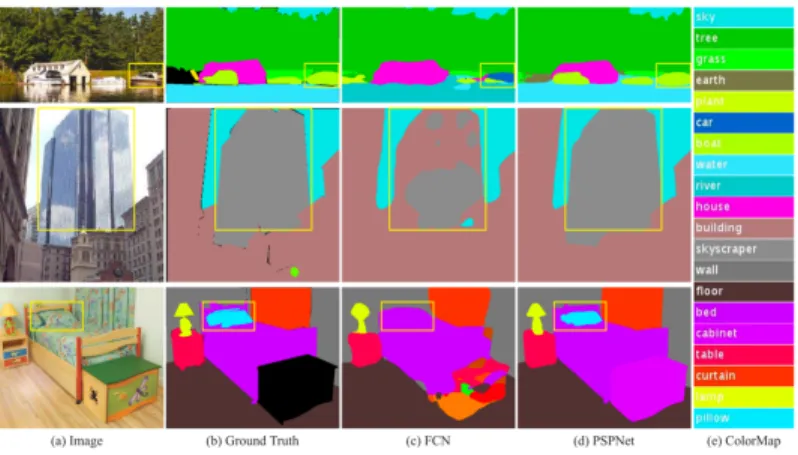
Furthermore, this direction has developed fast recently. PSPNet [28] has been proposed to further reuse different levels of features, which is designed to perform image segmentation on natural scenes. A comparison with other
Figure 2.7: PSPnet result comparison
networks could be shown in Fig. 2.7. The boundary and detection result of PSPNet is more smooth and accurate.
The trick of PSPNet is the design of fusion different level of features, i.e the feature map acquired by each Convolution Layer. As shown in 2.8, different sized feature map are supposed to have different level features. A combination of all these features could outperforms the previous design. However, how to design and fuse these layers are barely explained. The code published in Github is written in Caffe and contains 2000 lines for model definition, which leaves a hard job for people to understand. A detailed design of PSPnet could be seen in Fig. 2.9.
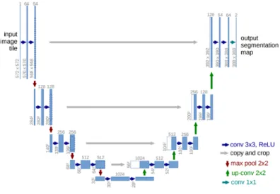
One important paper to mention is U-net [29], which is very famous in medical imaging segmentation working as a benchmark. The detailed design could be shown in 2.10. Although it used a small dataset to train model, Unet has been proved very powerful in many other scenarios. Learned from Residual
Figure 2.8: Design of PSPnet
Figure 2.10: Design of U-net
Network, each module in the figure below is a residual block containing several layers of Convnet and sampling. The novel idea here is not only build an auto-encoder, Unet will combine the output from the corresponding encoder with the input of the decoder as a new input into the next decoder layer. This design is hard to believe but turns out to be very useful by a series of related networks. U-net model has been widely applied and proved to be a success in the area of Medical Imaging on applications such as Lumbar Surgery[30] and gland segmentation[31].
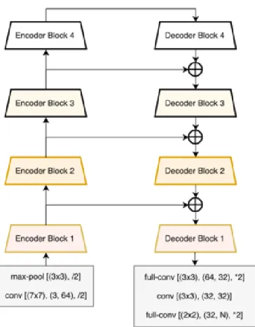
One step ahead, I would like to mention the LinkNet [32]. This is a very new paper just available in Arxiv. The network architecture could be seen below. In nature, it is very similar to U-net but it is designed with residual blocks. Input of each encoder layer is also bypassed to the output of its corresponding
Figure 2.11: Structure of Linknet
decoder. By doing this the model aims at recovering lost spatial information that can be used by the decoder and its upsampling operations. Such design could reduce parameters and be more efficient.
2.3.2
Conclusion
In this section, we go through the timeline of Encoder-Decoder based seg-mentation network structure. As we can see, there are two trends emerged in the development of Encoder-Decoder based models. The first is the reuse
of features to gain more information for segmentation. The second is reduce parameters to speed up.
For medical imaging, literatures published using such structure does not apply on the whole image but still a small patch of it. One possible reason is the medical image is too noisy. One possible solution is to make use of such model to generate a pixel-by-pixel prediction for each patch and using all the results as an input of the voting algorithm.
Figure 2.12: General Framework of GAN. GAN usually consists of two net-works: the Generator and the Discriminator. The Generator is trained to generate fake data samples from noises while the Discriminator network tries to discriminate fake data from the real data.
2.4
Generative Adversarial Network
Generative Adversarial Network (GAN) is a deep generative model proposed
by Goodfellow et al. [33], and later optimized by DCGAN [34] and WGAN [?].
The general framework is demonstrated in figure 2.12. There are two kinds of networks in GAN: the generator and the discriminator. The generator network is trained to fool the discriminator network, while the discriminator serves to distinguish whether an image is generated by the generator or is ground-truth. The generator and the discriminator are updated in parallel.
The goal of the Generator G is to learn a distributionpz matching the data, while the goal of Discriminator D is to distinguish the real data (i.e. from the real distributionpz) from the fake data generated by G. The adversarial comes
from the min-max game between G and D, which is formulated as:
min
G maxD V(D, G) =Ex∼pdata(x)[logD(x)] +Ez∼pz(z)[log(1−D(G(z)))], (2.7) where G tries to minimize this objective against an adversarial D that tries to maximize it.
However, the vanilla GAN suffers model collapse problem due to its loss design. To make the training process more stable, Arjovskyet al. [?] proposed Wasserstein GAN by using Earth Mover (EM) distance or Wasserstein-1 to evaluate the distance between the real distribution and the fake distribution [?]. Specifically, given two distributions, PdataandPz, with samplesx∼Pdata and y∼Pz, the Wasserstein-1 distance is defined as:
W(Pdata, Pz) = inf γ∈Q
(Pdata,Pz)E
(x,y)∼γ[kx−yk], (2.8)
where Q
(Pdata, Pz) denotes the set of all joint distributions γ(x, y) whose marginals are respectively Pdata and Pz. The term γ(x, y) could be viewed
as the cost from x to y in order to transform the distributions Pdata into
the distribution Pz. And the Wasserstein-1 loss actually indicates optimal
transport cost. Under this design, the loss for the G network is:
And the loss for the D network is:
LD =Ex∼Pz[D(G(x))]−Ex∼Preal[D(x)] (2.10)
2.4.1
Conclusion
In this section, we go through the design of GAN, which contains an Encoder and a Decoder. Starting with a minmax problem with two players, GAN takes advantage of game theory to train CNN get better performance. In another view, the design of GAN could be think of a new CNN based training loss, one other example could be the perceptron loss [35].
2.5
GAN Based Segmentation models
In this section, I will review related GAN based segmentation method. But this is a very new area and only two papers available at the moment, which is one area of great potential.
2.5.1
GAN for segmentation
Luc et al. [36] proposed a GAN based segmentation method which is shown in Fig. 2.13 . The model contains two parts, a segmentator and a discriminator. The segmentor is designed to generate a mask of the natural image, while the discriminator would decide if the generated mask the same as the ground truth mask. The quality of the generated mask is evaluated by how well it
Figure 2.13
is to fool the discriminator. The loss function is similar to the CGAN while some modification to consider the relationship between mask and the original
image. Given a data set of N training images xn and a corresponding label
mapsyn θs, θarepresenting the parameters of segmentor and advesarial model, the loss used in this model is shown in equation 2.11.
L(θs, θa) = N X n=1 L(s(xn), yn)−λ[bce((a(xn), yn),1) +bce((a(xn), s(xn)),0)], (2.11) where , a(x, y) ∈ [0,1] denotes the scalar probability with which the ad-versarial model predicts that y is the ground truth label map of x, as opposed
to being a label map produced by the segmentation models() And bce is the
binary cross-entropy loss, which is defined as:
The motivation for their approach is that, with the help of GAN, it can detect and correct higher-order inconsistencies between ground truth segmen-tation maps and the ones produced by the segmensegmen-tation net. The experiments show that their adversarial approach leads to improved accuracy on the Stan-ford Background and PASCAL VOC 2012 datasets.
Souly et al. [37] proposed two neutral frameworks for GAN based semi-supervised and weakly semi-supervised learning. The difference with [36] is it asked the Discriminator to generate mask instead of the Generator. Besides the original K classes of the segmentation task, one extra class, fake class, has been added for the discriminator so that it could decide whether the input is a fake one generated by the Generator. To ensure higher quality of generated images for GANs with consequent improved pixel classification, the second
framework extend the framework by adding weakly annotated data. This
greatly overcome the shortcoming of few labelled data is available.
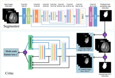
In the area of medical imaging, recently only one paper has been published related to GAN based segmentation. segAN [38] has been proposed, which is workflow is shown in 2.14. Since image segmentation requires dense, pixel-level labeling, the gradient feedback by the original GAN may not be enough for training, which has been mentioned in WGAN. To overcome this, a new loss is proposed by the design of adversarial critic network with a multi-scale L1 loss function to force the critic and segmentor to learn both global and
Figure 2.14: Structure of segAN
local features that capture long- and short-range spatial relationships between pixels. The loss proposed in this paper is very similar to the idea of EM loss used by WGAN.
GAN based lung segmentation
The image segmentation task in the area of medical imaging serves as the very first step of many tasks. For example, in the task of lung nodule detection or lung disease analysis, the segmentation of lung could remove many noise and reduce input size. Recently, in the low-dose CT reconstruction, since different types of tissue (e.g. fat, bone, muscle) have different texture, reconstruct each part separately could greatly improve the texture.
On the other hand, CNN based segmentation requires large amount of training data which is hard to acquire in the context of medical imaging. Small dataset may cause overfitting or failure in model training.
In this chapter, I will introduce one of such solution using Generative Ad-versarial Network to improve CNN based segmentation on the task of lung segmentation.
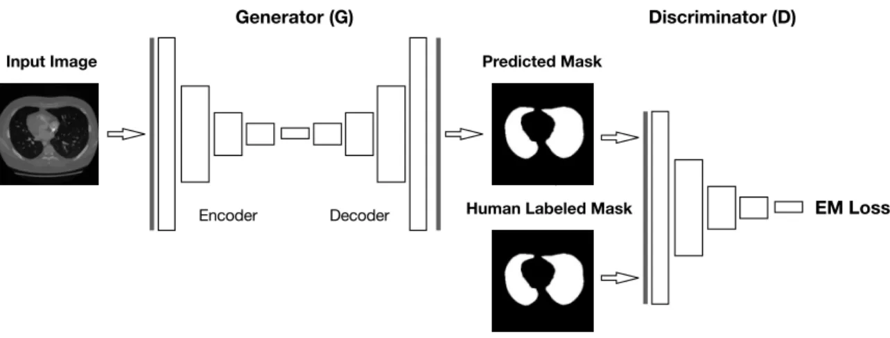
Encoder Decoder Generator (G) Input Image Discriminator (D) EM Loss Predicted Mask
Human Labeled Mask
Figure 3.1: The pipeline of the proposed LGAN schema which includes a generator network and a discriminator network. A Deep Deconvnet Network is trained to generate the lung mask while an Adversarial Network is trained to discriminate segmentation maps from the ground truth and the generator, which, in turn, helps the generator to learn an accurate and realistic lung segmentation of the input CT scans.
3.1
Background and motivation
Lung segmentation is an initial step in analyzing medical images obtained to assess lung disease. For example, early detection of lung nodules in lung cancer screening with CT is a tedious task for human readers and could be significantly improved with artificial intelligence. Researchers proposed a num-ber of lung segmentation methods which fall into two categories: hand-crafted feature-based methods and deep learning-based methods [39, 40, 41, 42]. Com-pared to the hand-crafted feature-based methods, such as region growing [41] and active contour model [42], deep learning-based methods could automati-cally learn useful features [43] without manually empirical parameter
adjust-ments.
Existing hand-crafted feature-based lung segmentation methods are usually performed through a series of procedures with manually empirical parameter adjustments. Various sets of 2D-based [40] and 3D-based methods [44] are developed to achieve a high quality segmented result.
However, these traditional segmentation techniques are designed for specific applications, imaging modalities, and even datasets. They are difficult to be generalized for different types of CT images or various datasets since different kinds of features and different parameter/threshold values are extracted from different datasets. Moreover, the feature extraction procedure is monitored by users and the features/parameters are analyzed and manually and interactively adjusted.
In this work, in contrast, we propose an end-to-end deep learning Gener-ative Adversarial Network (GAN) based lung segmentation schema (LGAN), where the input is a slice of lung CT scan and the output is a pixel-wise mask showing the position of the lungs by identifying whether each pixel belongs to lung or not. Furthermore, the proposed schema can be generalized to different kinds of networks with improved performance.
Recently, several deep learning-based pixel-wise classification methods have been proposed in computer vision area and some of them have been successfully applied in medical imaging. Early deep learning-based methods are based on
bounding box [16]. The task is to predict the class label of the central pixel(s) via a patch including its neighbors. Kallenberget al. [45] designed a bounding box based deep learning method to perform breast density segmentation and scoring of mammographic texture. The proposed model could learn a feature
hierarchy from unlabeled data. Shin et al. [46] compared several networks on
the performance of computer-aided detection and proposed a transfer learning method by utilizing models trained in computer vision domain for medical imaging problem. Instead of running a pixel-wise classification with a
bound-ing box, Long et al. [25] proposed a fully convolutional network (FCN) for
semantic segmentation by replacing the last part of the CNN which is usually fully connected layers, with convolutional layers to build a fully convolutional structure. After the coarse label map is obtained from the network, it is up-sampled with deconvolutional layers to yield per pixel classification results.
An Auto-Encoder alike structure has been used by Noh et al. [47] to
im-prove the quality of the segmented objects. With multiple up-pooling and deconvolutional layers in the architecture, the limitation of the fixed-size
re-ceptive field of FCN is eliminated. Later, Ronneberger et al. [48] proposed
a U-net model for segmentation, which consists of a contracting part as an encoder to analyze the whole image and an expanding part as a decoder to produce a full-resolution segmentation. The U-net architecture is different from [25] in that, at each level of the decoder, a concatenation is performed
with the correspondingly cropped feature maps from the encoder. This design has been widely used and proved to be successful in many medical imaging applications such as Lumbar Surgery[30] and gland segmentation[31]. Most recently, Lalonde et al. [49] designed a convolutional-deconvolutional capsule network, called SegCaps, to perform lung segmentation, where they proposed the concept of deconvolutional capsules.
After the emergence of Generative Adversarial Network (GAN) [33] based models, which have shown a better efficiency in leveraging the inconsistency of the generated image and ground truth in the task of image generation,
Luc et al. [36] proposed a GAN based semantic segmentation model. The
motivation is to apply GAN to detect and correct the high-order inconsistencies
between ground truth segmentation maps and the generated results. The
model trains a convolutional semantic segmentation network along with an adversarial network that discriminates segmentation maps coming either from the ground truth or from the segmentation network. Following this idea, Zhao et al. [50] proposed to use adversary loss to perform lung segmentation, where the segmentor is a fully convolutional neural network.
Both of their works utilize the original GAN structure, which, however, due to its loss function design, original GAN suffers from the problem of learning instability such as mode collapse, which means all or most of the generator outputs are identical [51, 52].
To avoid this problem, Arjovsky et al. [51] proposed an optimized GAN structure which uses a new loss function based on the Earth Mover (EM) distance and in the literature is denoted as WGAN. It should be noted that WGAN is designed to solve the same problem as the original GAN, which is to leverage the inconsistency of the generated image and ground truth in the task of image reconstruction instead of generating an accurate segmentation from a given type of images.
In this work, to solve the medical image segmentation problem, especially the problem of lung segmentation in CT scan images, we propose LGAN (Gen-erative Adversarial Network based Lung Segmentation) schema which is a gen-eral deep learning model for segmentation of lungs from CT images based on a Generative Adversarial Network (GAN) structure combining the EM distance based loss function. In the proposed schema, a Deep Deconvnet Network is trained to generate the lung mask while an Adversarial Network is trained to discriminate segmentation maps from the ground truth and the generator, which, in turn, helps the generator to learn an accurate and realistic lung seg-mentation of the input CT scans. The performance analysis on the dataset from a public database founded by the Lung Image Database Consortium and Image Database Resource Initiative (LIDC-IDRI) shows the effectiveness and stability of this new approach. The main contributions of this work include:
64 256 512 1024 256 128 64 1
conv1 conv2 conv3 conv4 conv5 conv6
H,W H/2,W/2 H/4,W/4 H/8,W/8 conv7 conv8 128 512 conv9 3 Grayscale Image X Segmentation Mask Y
Figure 3.2: The architecture of the generator in the framework. Each blue box represents the feature map generated by convolution block. The number of channels is denoted on the bottom of the box. The lines on the top of the boxes indicate the concatenation operation of the feature map.
Network (GAN) based lung segmentation schema (LGAN) with EM dis-tance to perform pixel-wised semantic segmentation.
2. We apply the LGAN schema to five different GAN structures for lung segmentation and compare with different metrics including segmentation quality, segmentation accuracy, and shape similarity.
3. We perform experiments and evaluate our five LGAN segmentation al-gorithms as well as the baseline U-net model using LIDC-IDRI dataset with ground truth generated by our radiologists.
4. Our experimental results show that the proposed LGAN schema out-performs current state-of-art methods on our dataset and debuts itself as a promising tool for automatic lung segmentation and other medical imaging segmentation tasks.
3.2
Method
In this section, we first introduce the background knowledge of Generative Adversarial Network and then present the proposed LGAN schema.
3.2.1
Generative Adversarial Networks
As introduced, a general GAN model consists of two kinds of networks named as the generator network and the discriminator network. The generator net-work is trained to generate an image similar to the ground-truth and mean-while the discriminator network is trained to distinguish the generated image from the ground-truth image. By playing this two-player game, the results from the discriminator network help the generator network to generate more similar images and simultaneously the generated images as the input data help the discriminator network to improve its differentiation ability. Therefore, the generator network and the discriminator network are competing against each other while at the same time make each other stronger.
Mathematically, the goal of the generator network Gis to learn a distribu-tion pz matching the ground-truth data in order to generate the similar data, while the goal of discriminator network D is also to learn the distribution of the ground-truth data but for distinguishing the real data (i.e. from the real
distribution pdata) from the generated data from G. The adversarial comes
min
G maxD V(D, G) =Ex∼pdata(x)[logD(x)]+Ez∼pz(z)[log(1−D(G(z)))], (3.1) where, for a given real data xand the corresponding generated data G(z), the adversarial discriminator is trained to maximize the probability output for the real data x (that is, Ex∼pdata(x)[logD(x)]) and minimize the probability
output for the generated data (that is, Ex∼pdata(x)[logD(G(z))]) which is
equiva-lent to maximizing Ez∼pz(z)[log(1−D(G(z)))], and on the other side, the generator
is trained to generate G(z) as similar as possible to x so that the discrim-inator outputs the bigger probability value for G(z), that is, to maximize
Ex∼pdata(x)[logD(G(z))] and equivalently minimize Ez∼pz(z)[log(1−D(G(z)))].
Luc et al. [36] adapt GAN model to perform segmentation task, where the role of the generator has been changed from generating synthetic images to generating segmentation masks given the original images, which has been proved to be effective on the task of lung segmentation by Zhao et al [50]. The details of GAN based segmentation design will be specified in the next section.
To make the training process more stable, Arjovskyet al. proposed WGAN
using EM distance to measure the divergence between the real distribution and the learned distribution [51]. Specifically, given the two distributions,Pdataand
Pz, with samples x∼Pdata and y ∼Pz, the EM distance is defined as:
W(Pdata, Pz) = inf γ∈Q
(Pdata,Pz)E
whereQ
(Pdata, Pz) represents the set of all joint distributionsγ(x, y) whose marginals are respectively Pdata and Pz, and the term γ(x, y) represents the cost fromxtoyin order to transform the distributions Pdatainto the distribu-tionPz. The EM loss actually indicates optimal transport cost. In this design, the loss for the generator network is:
LG =−Ex∼Pz[D(x)]. (3.3)
And the loss for the discriminator network is:
LD =Ex∼Pz[D(G(x))]−Ex∼Preal[D(x)]. (3.4)
With the EM distance based loss, the GAN model becomes more power-ful in generating high-quality realistic images and outperforms other gener-ative models. While the WGAN is designed for image reconstruction, here we take advantage of the basic idea of WGAN, and design an efficient and enhanced deep learning Generative Adversarial Network based Lung Segmen-tation (LGAN) schema.
3.2.2
Our LGAN Schema
Our Generative Adversarial Network based Lung Segmentation (LGAN) schema is designed to force the generated lung segmentation mask to be more consis-tent and close to the ground truth and its architecture is illustrated in Fig.
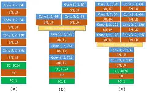
Figure 3.3: The architecture of different D networks, where Conv stands for
convolution layer, FC stands for fully-connected layer, BN stands for Batch
Normalization and LR stands for LeakyReLU. For each convolution layer,
the numbers means kernel size, (down) pooling stride and number of kernels accordingly. Feature concatenation layer combines feature maps from different branches.
3.1.
LGAN consists of two networks: the generator network and the discrimina-tor network, and all of them are convolution neural networks. The generadiscrimina-tor network is to predict the lung segmentation masks based on the grayscale in-put images of CT slices, while the discriminator comin-putes the EM distance between the predicted masks and the ground truth masks.
During the training and testing, the LGAN schema takes a slice of the lung CT scanIi as input, then the generator predicts a mask Mi to illustrate the pixels belong to the lung. The quality of lung segmentation is judged by
how well Mi fools the discriminator network. In the rest of this section, we describe the three main components of our LGAN schema: Generator Network, Discriminator Network, and Training Loss.
Generator Network
The generator network is designed to generate the segmented mask of the input lung CT scan image. The mask labels all the pixels belong to the lung. This segmentation task can be addressed as a pixel-wise classification problem to identify whether a pixel belongs to the lung area or not. Given an input CT slice Ii, the generator will predict the category of each pixel and generate a corresponding mask Mi based on the classification result.
The architecture of our designed generator is illustrated in Fig. 3.2. The generator model consists of encoder and decoder parts. The encoder extracts the high-level features from the input CT scan by a bunch of convolution blocks, while the decoder reconstructs the mask from the high-level features. Both encoder and decoder are composed of convolution blocks, which are rep-resented as blue boxes in the figure. The input of the generator network is normalized to 224×224 pixels and the generated mask is the same size as the input.
In the encoder part, each block has two convolution layers, both of which have the same number of filters with filter size 3×3 followed by a max-pooling
layer, which performs a 2×2 down-pooling on the feature map.
In the decoder part, each block consists of one deconvolution layer and two convolution layers. For the convolution layers, similarly, each has the same number of filters with filter size 3×3. Instead of an up-pooling layer, we use the deconvolution layer with stride 2 as suggested by Tran et al. [53] because deconvolution layer can generate better quality images than an up-pooling layer. Following other work, we add skip connection between the encoder and decoder.
Following DCGAN [34], we employ LeakRelu as the activation function for the convolution layers which is first proposed in [54]. As shown below, to alle-viate potential problems caused by ReLU, which sets 0 to all negative values, LeakyReLU set a small non-zero gradient NegativeSlope, which is user pre-defined, to negative values. In the equation below, we represent this negative slope as α.
LeakyReLU(x, α) = max(x,0) +α×min(x,0). (3.5)
At the final layer, a 1∗1 convolution is performed to map each component feature vector to the final segmentation mask.
Discriminative Network
The task of the discriminative network is to distinguish the ground truth mask from the generated segmentation mask. We employ the EM distance to
Table 3.1: The list of all the proposed five LGAN structures and their corre-sponding descriptions.
Network Input
LGANBasic generated mask, one at a time.
LGANP roduct segmented original image based on the predicted mask.
LGANEF mask and original image are combined as one input with two channels.
LGANLF mask and original image as two inputs.
LGANRegression generated mask and ground truth, so as to approximate EM loss directly.
measure the difference between the real and fake distributions as it has been proved to be a smooth metric [51].
Given a generator, the discriminator approximatesE[X] function such that the EM lossE[X]−E[Y] is approximated by D(G(z))−D(Real). Compared to the discriminator in the original GAN, which performs a classification task, the new discriminator is actually performing a regression task (approximating the function E(X)).
Based on the different assumptions that could help improve the perfor-mance of the discriminator network, we propose five different designs for the discriminator network, which thus yield five different LGAN structures. The details of the five frameworks are demonstrated in Tab. 3.1. We discuss these five designs one by one in the next section.
Training Loss
As the original WGAN is designed for image reconstruction tasks, here we
modify the training loss to fit for the segmentation task. Specifically, we
which calculates the cross-entropy between the generated mask and ground truth mask. Therefore, the loss of the generator network is:
BCE[G(x), Real]−Ex∼Pz[D(x)], (3.6)
Where Pz is the learned distribution from the ground-truth mask by G. For the training loss of the discriminator D, different designs for the dis-criminator network may have the different training loss functions which are described in the next section.
3.3
The Proposed LGAN Structures
In GAN-based image reconstruction tasks, the generated image and the ground truth image are very similar. However, for lung segmentation task, the pixel intensity in the generated mask is in [0,1] while the value in the ground truth mask is binary, that is, either 0 or 1. This fact may mislead the discriminator to distinguish the generated mask and the ground truth mask by simply detecting if the mask consists of only zeros and ones (one-hot coding of ground truth), or the values between zero and one (output of segmentation network).
With this observation, we explore all possible discriminator designs for lung segmentation task based on various assumptions, and provide five dif-ferent LGAN structures: LGAN with Basic Network, LGAN with Product Network, LGAN with Early Fusion Network, LGAN with Late Fusion
Net-work and LGAN with Regression NetNet-work. Their corresponding architectures are illustrated in Fig. 3.3. In the rest of this section, we introduce them ac-cordingly.
3.3.1
LGAN with Basic Discriminator
The basic discriminator is to evaluate the generated mask and the ground truth mask separately and minimize the distance between the two distributions, which can be illustrated as (a) in Fig. 3.3. We denote the LGAN with this basic discriminator asLGANBasicand it has a single channel with the network input size of 224×224.
InLGANBasic, the training loss ofGis the same as we described in section
3.2.2 and the training loss of D is the following:
Ex∼Pz[D(G(x))]−Ex∼Preal[D(x)]. (3.7)
Based on LGANBasic, we conjecture that the discriminator network may
have a more precise evaluation if the original image is also provided as addi-tional information. Under this assumption, we examine three strategies and
design the LGANP roduct, LGANEF, and LGANLF structures.
3.3.2
LGAN with Product Network
Different from the basic discriminator where the inputs are the segmented mask and the ground-truth mask with only binary value, the product network
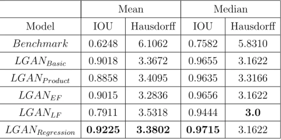
Table 3.2: Performance comparison of 2D-LGAN.
Mean Median
Model IOU Hausdorff IOU Hausdorff
Benchmark 0.6248 6.1062 0.7582 5.8310 LGANBasic 0.9018 3.3672 0.9655 3.1622 LGANP roduct 0.8858 3.4095 0.9635 3.3166 LGANEF 0.9015 3.2836 0.9656 3.1622 LGANLF 0.7911 3.5318 0.9444 3.0 LGANRegression 0.9225 3.3802 0.9715 3.1622
takes, as the inputs, the lung volume images which are mapped out from the original CT scan image by the segmented mask and the ground-truth mask respectively. That is, given the segmentation mask, we obtain the lung volume image by modifying the original image such that the values within the segmented lung area are kept as they are but the values in the rest of the area are set to be 0. This design is motivated by the work of Luc et al. [36].
With this input, the discriminator network might be biased by the value distribution. Although in [36] the deep learning model with the product net-work is not designed based on WGAN, we observe that the product netnet-work could still be used in our LGAN model and we define this LGAN structure
as LGANP roduct. Note that the discriminator in LGANP roduct differs from
LGANOrigin only in inputs, so the discriminator in LGANP roduct shares the
same architecture as LGANOrigin shown in (a) of Fig. 3.3.
and the training loss of D, which is product network, is the following:
Ex∼Pz[D(G(x)◦Ii)]−Ex∼Preal[D(x)], (3.8)
where x ◦y is a pixel-wise multiplication of matrixx and y, and the mask and the original image has the same size.
3.3.3
LGAN with Early Fusion Network
Instead of taking only the mask as inputs, early fusion network takes both the whole original CT scan image and the segmentation/ground-truth mask as an input. To keep the design of single input, we concatenate the original image and the mask as one single image with two channels, where one channel is the
original CT scan and the other is the mask. We denote LGAN with this early
fusion discriminator network as LGANEF.
The architecture of the discriminator inLGANEF is shown in (a) of Fig.3.3.
Different from LGANBasic and LGANP roduct, LGANEF has the input size of
224×224 with 2 channels which are the concatenation of the original CT scan and its mask. In LGANEF, the training loss of G is the same as we described in section 3.2.2 and the loss of the discriminator network is:
Ex∼Pz[D(G(x) M Ii)]−Ex∼Preal[D(x) M Ii], (3.9) wherexL
a single matrix with 2 channels.
3.3.4
LGAN with Late Fusion Network
Another way of taking both the original image and the mask as an input in the discriminator network is to employ the late fusion technique. Specifically, the input of the discriminator is the concatenation of the high-level feature of the CT scan and the mask. We denote LGAN with this type of discriminator
as LGANLF.
The corresponding architecture of the discriminator in LGANLF is shown
in (b) of Figure 3.3. There are two branches of convolution operations in this discriminator. One is for the CT scans, and the other is for the masks. The two inputs first pass the two branches separately, and then their features are fused by a concatenate layer and pass through several convolut
![Figure 2.4: The method proposed by Zeiler et al. [1], as shown in figure, this is how to reverse the operation of convolution with ReLU as activation function followed by down-sampling.](https://thumb-us.123doks.com/thumbv2/123dok_us/371448.2540924/40.918.262.665.335.754/figure-proposed-operation-convolution-activation-function-followed-sampling.webp)