Archive of SID
Iranian Journal of Science & Technologyhttp://www.shirazu.ac.ir/en
Resource allocation in multi-server dynamic PERT networks using
multi-objective programming and Markov process
S. Yaghoubi
1, S. Noori
1and M. Bagherpour
1*
1
Department of Industrial Engineering, Iran University of Science and Technology, Tehran, Iran E-mail: [email protected]
Abstract
In this research, both resource allocation and reactive resource allocation problems in multi-server dynamic PERT networks are analytically modeled, where new projects are expected to arrive according to a Poisson process, and activity durations are also known as independent random variables with exponential distributions. Such system is represented as a queuing network, where multi servers at each service station are allocated, and also each activity of a project is operated at a devoted service station with only one server located at a node of the network based on First Come First Serve (FCFS) policy. In order to propose a novel approach for modeling of multi-server dynamic PERT network, initially the network of queues is transformed into a stochastic network. Then, a differential equations system is organized to solve and obtain approximate completion time distribution for any particular project by applying an appropriate finite-state continuous-time Markov model. Finally, a multi-objective model including four conflicted objectives is presented to optimally control the resources allocated to the service stations in a multi-server dynamic PERT network, and the goal attainment method is further employed to solve a discrete-time approximation of the primary multi-objective problem.
Keywords:Project management; Markov processes; multiple objective programming; reactive resource allocation
1. Introduction
Some organizations are project-oriented based and operate their activities depending on projects. In such situations, the organizations may carry out the multi project concurrently, whereas, Payne [1] revealed that up to 90% organizations execute the projects in a multi-project environment. Commonly, the limited resources are shared and competed among multiple projects for achieving their own goals.
Therefore, multi-project management system is a vital approach in project scheduling and management, whereas traditional project scheduling has been concerned mostly with single project optimization. Multi-project resource constrained scheduling problem (MPRCSP) is the main topic of most investigations on multi-project scheduling considering static and deterministic environments. Pritsker et al. [2] by using a zero-one integer programming approach and Wiest [3] by presenting an heuristic model, analyzed the MPRCSP. Then, Kurtulus and Davis [4] and Kurtulus and Narula [5] by applying priority rules and defining measures such as the rate of utilization of each resource type and the peak of total resource requirements, studied the MPRCSP.
*Corresponding author
Received: 25 April 2010 / Accepted: 30 August 2010
Also, multi criteria and multi objective modeling is then used in MPRCSP. For example, a 0–1 goal programming is applied by Chen [6] in multi-project resource-constrained scheduling for the maintenance of mineral processes, and a lexicographicly two criteria is presented by Lova et al. [7]. Recently, scheduling rules in the static MPRCSP environment were presented by Kanagasabapathi et al. [8] considering performance measures involving mean tardiness and the maximum tardiness of projects involved.
Moreover, heuristic & meta-heuristic algorithms for analyzing MPRCSP were applied [9-14]. Recently, MPRCSP was extended by considering transfer times and its relevant costs by Kruger and Scholl [15].
In the literature, MPRCSP was mostly analyzed on static and deterministic environments and a few investigations have been focused on multi-project scheduling under uncertainty and dynamic conditions. A simulation model for multi-project resource allocation with stochastic activity, as a multi-channel queuing, was presented by Fatemi-Ghomi and Ashjari [16]. Also, a nonlinear mixed-integer programming model for optimizing the multi project resource allocation was proposed by Nozick et al. [17], whereas changing resource allocations affects the probability distribution of activity duration. An event-driven approach was
Archive of SID
represented by Kao et al. [18], and also, usingCritical Chain Project Management (CCPM) approach, the uncertainty in multi project system was studied by Byali and Kannan [19]. MPRCSP is commonly analysed by either connecting them together into a large single project by the addition of dummy start and end activities or considering the projects as independent and linking them by using an objective function which contains each project individually (probably with appropriate weigh factors) and the corresponding resource constraints.
In many organizations, not only are the activity durations uncertain, but also, new projects dynamically arrive to the project based organizations over the time horizon. Clearly, in this condition, project scheduling procedure would be more difficult and more complex than before. This problem, considered in project-oriented organizations, was studied by Adler et al. [20] by applying simulation. In this investigation, the organization was presented as a “stochastic processing network” with a collection of service stations (work stations) or resources, where one or more identical “servers” for serving projects under a pre-specified discipline, has been settled at each station. The represented organization can be expressed as a queuing network (dynamic PERT network), where each activity is getting the required services, queuing up for access to a resource, or waiting to join a predecessor activity. Such problem is attractive for organizations with similar projects, for example, maintenance projects in which a typical project will be repeated.
Also, the concept of CONWIP (constant work-in-process) is employed by Anavi-Isakow and Golany [21] in dynamic PERT network for controlling projects using simulation study. Authors presented two control mechanisms: CONPIP (COnstant Number of Projects In Process) that limits the number of projects, and CONTIP (CONstant Time of projects In Process), that restricted the total processing time of all active projects. A risk element was considered in dynamic PERT network by Li and Wang [22] and a multi-objective risk-time-cost trade-off problem was proposed based on general project risk element transmission theory.
Through resource allocation problem in dynamic PERT network, two commonly used approaches exist. The first approach was propounded by Cohen et al. [23, 24], where the resources may work in parallel, i.e., the number of servers and resources allocated in every service station are equal (e.g., electrical work station with electricians, mechanical work station with mechanics, etc.) and the amount of resources available to be allocated to all service stations is constant. They presented near optimal resource allocated to the entities that perform the projects in CONPIP system by using Cross Entropy
(CE) based on simulation. We denominate this approach as “resources as servers” and in this article, based on this approach a multi-objective model will be proposed.
In the second approach, investigated by Azaron and Tavakkoli-Moghaddam [25], the number of servers in every service station is fixed and resources allocated affect the mean of service times.
Authors presented an analytical multi-objective model for the resource allocation problem in a dynamic PERT network and assumed the activity durations are exponentially distributed random variables, the new projects are generated according to a Poisson process, the number of servers in every service station is either one or infinity and the capacity of the system is infinite. Recently, Yaghoubi et al. [26] modeled the resource allocation problem in dynamic PERT networks, where the capacity of system is finite and projects are generated according to a Poisson process. We denominate this approach as “resources affecting servers” and in this article, based on this approach a multi-objective model is proposed.
In both approaches, the uncertainty is considered in the entrance of projects and also in the duration of service stations, whereas other uncertainty such as project network disruption may happen. In this research, for avoiding project network disruption, “reactive resource allocation” is suggested. Along with the project execution, a project may be disposed by considerable unforeseen disruptions, therefore, reactive scheduling (rescheduling), with revising or re-optimizing the initial baseline schedule, aims to adjust the baseline schedule and consequently, overcome the disruptions.
Firstly, reactive scheduling was propounded in manufacturing environments and then it was applied through project scheduling approaches. Comprehensive investigations about reactive scheduling in manufacturing environments have been studied [27-32]. Vieira et al. [29], based on wide variety of experimental and practical investigations, introduced a framework of strategies, policies and methods for reactive scheduling and Aytug et al. [30] by defining different types of uncertainties, proposed a review of rescheduling based approaches. Herroelen and Leus [31] represented the basic aspects for scheduling under uncertain conditions: reactive scheduling, stochastic project scheduling, fuzzy project scheduling, robust (proactive) scheduling and sensitivity analysis. Also, Van de Vonder et al. [32], based on practical design, analysed several predictive-reactive resource-constrained project scheduling procedures.
Various approaches exist in the literature of the reactive scheduling problems. A simple and initial approach is a right shift rule that is removed ahead
Archive of SID
in time of all the affected activities [33]. Fullrescheduling, the other approach, considers the remainder of activities that are to be completed. The other important approach is minimum perturbation strategy which applies the exact and suboptimal method for minimizing the difference between the revised schedule and the primary schedule [34-36]. Recently, Liu and Shih [37], based on a primary schedule and actual progress, studied resource-constrained construction rescheduling and suggested a new rescheduling optimization model using constraint programming, also, Novas and Henning [38] introduced the repair-based reactive scheduling of industrial batch plants.
Reviewing the above mentioned researches indicated no closely related work was found to analytically analyze multi-server dynamic PERT networks. As the main contribution of this research, we develop a novel approach for the resource allocation problem (or time-cost trade off problem) and also reactive resource allocation problem in multi-server dynamic PERT networks by means of multi- objective programming and Markov process. Through this investigation, we consider a multiple environment and concurrent projects including new projects, containing all the activities that arrive at the system according to an independent Poisson process. It is also assumed each activity of the projects is performed at a devoted service station located at a node of the network with FCFS policy. It is further assumed different servers are allocated in each service station, while the services processing times (or activity durations) are followed as independently random variables with exponential distributions.
For modeling a multi-server dynamic PERT network, firstly, for obtaining the states of a system, the network of queues is transformed into a stochastic network. Then, a system of differential equations is organized to solve and obtain the approximate completion time distribution for any particular project by creating an appropriate finite-state continuous-time Markov model. Finally, a multi-objective model with four conflicted objectives is presented to optimally control the resources allocated to service stations in a multi-server dynamic PERT network, and the goal attainment method is finally employed to solve a discrete-time approximation of the primary multi-objective problem.
This paper is comprised of five sections. The remainder is organized as follows. In Section 2, we model the multi-server dynamic PERT network by employing a finite-state continuous-time Markov process and propose a multi-objective model to optimally control the resources allocated to service stations in a multi-server dynamic PERT network. In Section 3, reactive resource allocation in the
multi-server dynamic PERT network is discussed. We solve an illustrative case in Section 4, and the conclusion is given in Section 5.
2. Multi-server dynamic PERT network
In this section, the multi-server dynamic PERT network is modeled to optimally control the resources allocated to the corresponding activities. Also, an analytical method to compute the approximate distribution function of project completion and a objective model in a multi-server dynamic PERT network are presented.
2.1. Continuous-time Markov process
For modeling the multi-server dynamic PERT network, we use the method presented by Kulkarni and Adlakha [39]. This is the reason this method is an analytical approach, simple, easy to implement through a computer, and is computationally stable. It is assumed that a project is represented as an Activity-on-Node (AoN) structure, also new projects, containing all the activities, arrive at the multi project system according to a Poisson process at the rate of . Furthermore, each activity of the project is executed at a devoted service station settled in a node of the network based on FCFS policy, where the service time (activity duration) is exponentially distributed.
Such system can be considered as a network of queues, where the arrival stream of projects to each service station is followed according to a Poisson process with the rate of , and the service times are the durations of the corresponding activities. It is assumed that service processing times in service station a are exponentially distributed at a rate of
a
and the number of servers in node a is ma. So
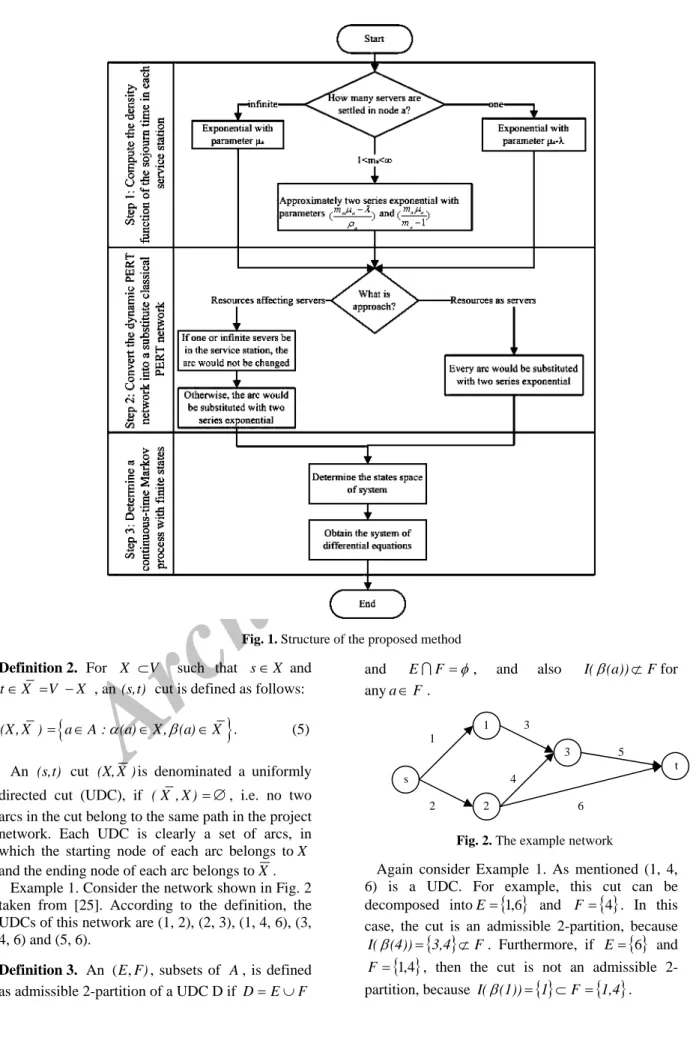
the node a is treated as an M /M /ma model. The flow chart of our proposed method for multi-server dynamic PERT network is presented in Fig. 1. To continue the steps of our proposed method for multi-server dynamic PERT network as continuous-time Markov process is extensively explained: Step 1. Compute the density function of the sojourn time (waiting time plus activity duration) in each service station. (see appendix A)
Step 1.1. If ma 1, then the queueing system would be an M/M/1 queue, and the density function of time spent at the service stationa(wa(t))would be exponentially expressed with parameter a , therefore, wa( )t is
calculated as follows:
( )
( ) ( ). a t 0, 1
a a a
Archive of SID
Step 1.2. If ma , then the queueing system is
/ /M
M , and the density function of time spent in the service station a would be exponentially expressed with parameter a, therefore, wa( )t is
calculated as follows:
( ) . at 0,
a a a
w t e t if m (2) Step 1.3. If 1ma , then the queueing system is M/M/ma, and the density function of time
spent in the service station a would be approximately two series exponential with parameters ( a a ) a m and ( ) 1 a a a m m ,where a a a m . Therefore, wa(t) is approximately calculated as follows: ( ) ( ) 1 ( ) 1 ( ) ( )( ). ( ) ( ) 1 ( ) ( )( ) 0 1 ( ) ( ) 1 a a a aa a a a m t a a a a a a a a a a a a a m t m a a a a a a a a a a m m m w t e m m m m m e t m m m m (3)
Step 2. Convert the dynamic PERT network as an Activity-on-Node (AoN) structure into a substitute classical PERT network represented as an Activity-on-Arc (AoA) graph.
Step 2.1. By considering the AoN graph, substitute each node with a stochastic arc (activity) whose length is equal to the sojourn time in the corresponding service station.
For this purpose, node a in the AoN graph should be replaced with a stochastic activity. Assume b b1, 2,...,bn are the incoming arcs to node
a and d d1, 2,...,dm are the outgoing arcs from it.
Then, node a is substituted by activity ( ,v w), whose length is equal to the sojourn time in the service station a. Furthermore, all arcs b b1, 2,...,bn
terminate with node v while all arcs d1,d2,...,dm
begin from node w. (for more details, see [40]) Step 2.2. Transform the PERT network, obtained in step 2.1, into a new PERT network with exponentially distributed arc length.
Resources as servers approach: in this approach in which the number of servers and resources allocated in every service station are equal, every arc would be substituted with two series of
exponential arc with the parameters ( a a )
a m and ) 1 ( a a a m m
. After replacing all arcs with the
proper exponential two series arc, the PERT network obtained in step 2.1, is transformed into a new PERT network.
Resources affecting servers approach: in this approach, the number of servers in every service station is fixed and resources allocated affect the mean of service times. As mentioned in steps 1.1 and 1.2, If one or infinite severs be in the work station, then the length of arc would be exponential with parameters a and a, respectively, and
the corresponding arc would not be changed. But, if several servers (1ma ) be in the work station,
then the corresponding arc would be substituted with two series of exponential arc with the parameters ( a a ) a m and ( ) 1 a a a m m . After
replacing all such arcs with the proper exponential two series arc, the PERT network obtained in step 2.1, is transformed into a new PERT network.
Step 3. Determine a continuous-time Markov
process with finite states.
Step 3.1. Determine the states space of system. For this purpose, let G(V,A) be the PERT network, obtained in step 2.1, with a single source and a single sink, in which V represents the set of nodes and A represents the set of arcs of the network in the AoA network. Also, let G(V,A)
be a new PERT network, obtained in step 2.2, in which V represents the set of nodes and A
represents the set of arcs of the network in a new AoA graph. Let s and t be the source and sink nodes in the new PERT network, respectively, and the length of arc aA be a random variable that is exponentially distributed with parameter a. For
aA, the starting node and the ending node of arc a, are denoted as (a) and (a), respectively. Henceforth in this section, we analyze the new PERT network to determine a continuous-time Markov process with finite state space.
Definition 1. Let I(v) be the set of arcs ending at node
v
and O(v) be the set of arcs starting at nodev
in the new PERT network, which are defined as follows: (see [39])
( ), ( ). I (v) a A : (a) v v V O (v) a A : (a) v v V (4)Archive of SID
Fig. 1. Structure of the proposed method
Definition 2. For X V such that sX and
tX V X , an (s,t) cut is defined as follows:
.(X , X ) aA : (a) X , (a) X (5) An (s,t) cut (X,X)is denominated a uniformly directed cut (UDC), if ( X , X ) , i.e. no two arcs in the cut belong to the same path in the project network. Each UDC is clearly a set of arcs, in which the starting node of each arc belongs toX
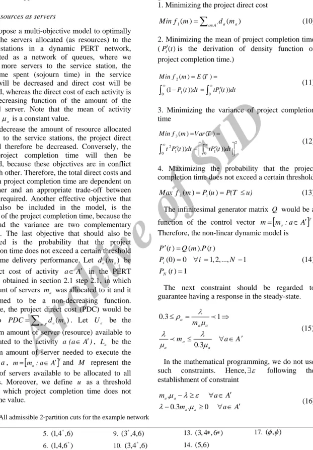
and the ending node of each arc belongs toX. Example 1. Consider the network shown in Fig. 2 taken from [25]. According to the definition, the UDCs of this network are (1, 2), (2, 3), (1, 4, 6), (3, 4, 6) and (5, 6).
Definition 3. An (E,F), subsets of A, is defined as admissible 2-partition of a UDC D if DEF
and EF , and also I((a))Ffor anyaF.
Fig. 2. The example network
Again consider Example 1. As mentioned (1, 4, 6) is a UDC. For example, this cut can be decomposed intoE
1,6 and F
4 . In this case, the cut is an admissible 2-partition, because
3,4 F(4))
I( . Furthermore, if E
6 and
1,4
F , then the cut is not an admissible 2-partition, because I((1))
1 F
1,4 . s t 1 2 3 1 2 3 4 5 6Archive of SID
Definition 4. Along with the project execution attime t, each activity (arc) can be in one and only one of the active, dormant or idle states, which are defined as follows:
(i) Active: an activity a is active at time t if it is being performed at time t.
(ii) Dormant: an activity a is called dormant at time t if it has completed but there is at least one unfinished activity in I((a)) at time t.
(iii) Idle: an activity a is denominated idle at time t if it is neither active nor dormant at time
t.
Also, Y(t) and Z(t) are defined as follow:
: , : , Y (t) a A a is active at time t Z (t) a A a is dormant at time t (6) and X(t)(Y(t),Z(t)).All admissible 2-partition cuts of the network of Fig. 2 are presented in Table 1. A superscript star is applied to denote a dormant activity and all others are active. E and F contain all active and all dormant activities, respectively.
The set of all admissible 2-partition cuts for the network are defined as S and also S S
(,)
. Note that X(t)(,) presents that the all activities are idle at time t and therefore the project is finished by time t. It is demonstrated that
X(t),t0
is a finite-state absorbing continuous-time Markov process. (for more detail, see [38])Step 3.2. Obtain the system of differential equations.
As previously mentioned, a UDC is divided into
E and F that contain active and dormant activities, respectively. If activity a terminates (with the rate of a), and I((a))F
a , thereis at least one unfinished activity in ( ( ))I a , then
,
E E a F F a . Furthermore, if by completing activity a, all activities in ( ( ))I a
become idle ( ( ( ))I a F
a
), then
( ) ( ( ))
E E a O a , F F I( ( )) a . Namely, all activities in I((a)) will become idle and also the successor activities of this activity,
)) ( ( a
O , will become active. Therefore, the components of the infinitesimal generator matrix
q(E,F),(E,F)
Q , (E,F)and (E,F)Sare obtained as follows:
0 ) , ( ), , ( E a a a a F E F E q (7)
a E E
a F F
a F a I E a if : , (( )) , ,
: , ( ( )) , ( ) ( ( )), ( ( )) if a E I a F a E E a O a F F I a F F E E if : , otherwise
X(t) ,t0 is a continuous-time Markov process with finite state space__
S and since
( , ),( , )
0q , the project is completed. In this Markov process all of the states except
) , ( ) (t
X which is an absorbing state, are transient. Furthermore, the states in S should be numbered such that this Q matrix be an upper triangular one. It is assumed that the states are numbered as 1,2,...,N S so that X(t)(O(s),)
and X(t)(,) are state 1 (initial state) and state N (absorbing state), respectively.
Let T be the length of the longest path or the project completion time in the new PERT network, obtained in step 2.2. Obviously,
min
T t 0 : X (t) N X (0)1 .
Chapman–Kolmogorov backward equations can be used to calculate F(t)P(T t). If it is defined
( ) ( 1, 2,...,
i
P t P X (t) N X (0) i ) i N, (8)
then F(t)P1(t).
The system of linear differential equations for the vector P(t)
P1(t) P2(t) .... PN(t)
Tis presented as follows:
( ) ( ) . ( ) .... T , dP t P t Q P t dt P(0) 0 0 1 (9)where P(t) and Q represent the derivation of the state vector P(t) and the infinitesimal generator matrix of the stochastic process
X (t) , t 0
, respectively.2.2. Multi-objective resource allocation
In this paper, following the research presented by Azaron and Tavakkoli-Moghaddam [25], we propose a multi-objective model to optimally
Archive of SID
control the resources allocated to the servicestations in a dynamic PERT network based on the mentioned two approaches.
2.2.1. Resources as servers
We propose a multi-objective model to optimally control the servers allocated (as resources) to the service stations in a dynamic PERT network, represented as a network of queues, where we allocate more servers to the service station, the mean time spent (sojourn time) in the service station will be decreased and direct cost will be increased, whereas the direct cost of each activity is a non-decreasing function of the amount of the allocated server. Note that the mean of activity duration a is a constant value.
If we decrease the amount of resource allocated (servers) to the service stations, the project direct cost will therefore be decreased. Conversely, the mean project completion time will then be increased, because these objectives are in conflict with each other. Therefore, the total direct costs and the mean project completion time are dependent on each other and an appropriate trade-off between them is required. Another effective objective that should also be included in the model, is the variance of the project completion time, because the mean and the variance are two complementary concepts. The last objective that should also be considered is the probability that the project completion time does not exceed a certain threshold for on-time delivery performance. Let da(ma) be
the direct cost of activity aA in the PERT network, obtained in section 2.1 step 2.1, in which the amount of servers ma was allocated to it and it
is assumed to be a non-decreasing function. Therefore, the project direct cost (PDC) would be equal to PDC
aAda(ma). Let Ua be themaximum amount of server (resource) available to be allocated to the activity a(aA), La be the
minimum amount of server needed to execute the activity a,
Ta:a A
m
m and M represent the amount of servers available to be allocated to all activities. Moreover, we define u as a threshold value in which project completion time does not exceed the value.
Therefore, this is a multi-objective stochastic programming problem. The objective functions are given as follows:
1. Minimizing the project direct cost
1( ) a A a( a)
Min f m
d m (10) 2. Minimizing the mean of project completion time (P1(t)is the derivation of density function of project completion time.)2 1 1 0 0 ( ) ( ) (1 ( )) ( )) Min f m E T P t dt tP t dt
(11)3. Minimizing the variance of project completion time 3 2 2 1 1 0 0 ( ) ( ) ( )) ( )) Min f m V ar T t P t dt tP t dt
(12) 4. Maximizing the probability that the project completion time does not exceed a certain threshold4( ) 1( )
Max f m P u P(T u) (13) The infinitesimal generator matrix Q would be a function of the control vector m
ma:aA
T.Therefore, the non-linear dynamic model is ( ) ( ). ( ) (0) 0 1, 2,..., 1 ( ) 1 i N P t Q m P t P i N P t (14)
The next constraint should be regarded to guarantee having a response in the steady-state.
0.3 1 0.3 a a a a a a m m a A (15)
In the mathematical programming, we do not use such constraints. Hence, following the establishment of constraint A a m A a m a a a a 0 . 3 . 0 . (16)
Table 1. All admissible 2-partition cuts for the example network
1. (1,2) 5. (1,4*,6) 9. (3*,4,6) 13. (3, 4 , 6 ) 17. (,) 2. (2,3) 6. (1,4,6*) 10. (3,4*,6) 14. (5,6) 3. (2,3*) 7. (1,4*,6*) 11. (3,4,6*) 15. (5*,6) 4. (1,4,6) 8. (3,4,6) 12. (3*,4,6*) 16. (5,6*)
Archive of SID
Consequently, the appropriate multi-objectiveoptimal control problem is expressed as below:
1( ) a( a) a A Min f m d m
2( ) 0 1( )) Min f m
tP t dt 2 2 3 1 1 0 0 ( ) ( )) ( )) Min f m t P t dt tP t dt
4( ) 1( ) Max f m P u ( ) ( ). ( ) P t Q m P t (0) 0 1, 2,..., 1 ( ) 1 i N P i N P t (17) . 0.3 . 0 a a a a m a A m a A a a a a m L a A m U a A a a A m M
int a m is eger a AThis continuous-time stochastic programming is impossible to solve (for more details see [25]), therefore, based on the definition of integral thinking, we divide the time interval into R equal portions with the length of t. Indeed, we transform the differential equations into difference equations. Thus, the corresponding discrete state model can be given as follows:
A a a a m d m f Min 1( ) ( )
1 0 1 1 2( ) ( ( 1) ( )) R r r P r P t r m f Min 1 2 3 1 1 0 2 1 1 1 0 ( ) ( ) ( ( 1) ( )) ( ( 1) ( )) R r R r Min f m r t P r P r r t P r P r
t u P m f Max 4( ) 1 : .t s P(r1)P(r)Q(m)P(r)t r0,1,2,...,R1R r N i r P R r r P N i P i N i ,..., 2 , 1 , 1 ,..., 1 , 0 1 ) ( ,..., 1 , 0 1 ) ( 1 ,..., 2 , 1 0 ) 0 ( (18)
A a m A a m a a a a 0 . 3 . 0 .
A a U m A a L m a a a a
m M A a a
maisinteger aA
2.2.2. Resources affecting servers
In this section, we propose a multi-objective to optimally control the resources allocated to the service stations based on resources affecting servers approach in a multi-server dynamic PERT network, represented as a network of queues. The direct cost of each activity is a non-decreasing function and the mean service time in each service station is a non-increasing function of the amount of resource allocated to it.
Let xa be the resource allocated in service station
a (aA), also da(xa) be the direct cost of
activity aA in the PERT network, obtained in section 2.1 step 2.1, while it is assumed to be a non-decreasing function of amount of resources xa
allocated to it. Thus, the project direct cost (PDC) would be PDC
aA/da(xa). Also, the meanservice time in the service station aA, ga(xa)
is assumed to be a non-increasing function of the amount of resource xa allocated to it that would be
equal to 1 ( ) a a a g x a A (19) Let Ua be the maximum amount of resource
available to be allocated to the activity a(aA),
a
L be the minimum amount of resource needed to execute the activity a, x
xa:aA
T and Jrepresent the amount of resource available to be allocated to all of activities. Moreover, we define u as a threshold time that project completion time does not exceed. Let B be the set of arcs in the PERT network, obtained in section 2.1 step 2.1, where there are infinite servers settled on the corresponding service station. The next constraint should be satisfied to keep the response in the steady-state. . 0.3 . 0 a a a a a m a A B m a A B a B (20)
In practice, da(xa) and ga(xa)can be obtained
by employing linear regression based on the previous similar activities or applying the judgments of experts in this area.
Consequently, the appropriate multi-objective optimal control problem is:
Archive of SID
1( ) a( a) a A Min f x d x
2( ) 0 1( )) Min f x
tP t dt 2 2 3( ) 0 1( )) 0 1( )) Min f x t P t dt tP t dt
4( ) 1( ) Max f x P u : .t s P t( )Q x P t( ). ( )(0) 0 1, 2,..., 1 ( ) 1 i N P i N P t a( a) 1 a g x a A (21)
. 0.3 . 0 a a a a a m a A B m a A B a B
a a a a x L a A x U a A
a a A x J
We divide the time interval into R equal portions with the length of t. The corresponding discrete state model as follows
1( ) a( a) a A Min f x d x
1 2 1 1 0 ( ) ( ( 1) ( )) R r Min f x r t P r P r
1 2 3 1 1 0 2 1 1 1 0 ( ) ( ) ( ( 1) ( )) ( ( 1) ( )) R r R r Min f x r t P r P r r t P r P r
t u P x f Max 4( ) 1 (22) : .t s P(r1)P(r)Q(x)P(r)t r0,1,2,...,R1 (0) 0 1, 2,..., 1 ( ) 1 0,1,..., ( ) 1 0,1,..., 1, 1, 2,..., i N i P i N P r r R P r i N r R a( a) 1 a g x a A . 0.3 . 0 a a a a a m a A B m a A B a B a a a a x L a A x U a A a a A x J
2.3. Goal attainment method
We now need to apply a multi-objective method to solve the proposed models, and we actually apply goal attainment technique for this purpose. Assume there is a multi-objective programming with n objectives, see (23), where fj(x) and X
are jth objective and feasible region of the problem, respectively. 1( ), 2( ),..., ( ) . : n Min f x f x f x s t xX (23)
The goal attainment method requires determining a goal, bj, and a weight, cj, for every objective.
j
c ’s reflect the importance of objectives, whereas if an objective has the smallest cj, then it will be the
most important objective. cj’s (j1,2,...,n) are
commonly normalized such that 1 1
n j j c .Therefore, the appropriate goal attainment formulation of the multi-objective problem is given by . : j( ) j j 1, 2,..., Min z s t f x c z b j n x X (24)
For solving the multi-objective models proposed in section 2.2 with the goal attainment method, the goals, bj’s, and weights, cj’s (j1,2,3,4), should
be determined for every objective, namely, the project direct costs, the mean of project completion time, the variance of project completion time and the probability that the project completion time does not exceed a certain threshold. Then, by applying (24) the appropriate goal attainment formulation of the multi-objective problem should be formed.
3. Reactive resource allocation in multi-server dynamic PERT networks
In the previous section, a multi-objective model for the resource allocation in multi-server dynamic PERT network was proposed. In the presented model, the uncertainty was considered in the entrance of projects and also in the duration of service stations, whereas, other uncertainty as project network disruption can occur. In this section, project network disruption such as: inserting a new activity (service station), deleting an activity and changes in precedence relations of project are considered. For coping with project network disruption, “reactive resource allocation”
Archive of SID
is also suggested. Along with the project execution,a project may be disposed the considerable unforeseen disruptions, therefore, reactive scheduling (rescheduling), with revising or re-optimizing the baseline schedule, aims to repair the baseline schedule and consequently, overcome disruptions.
For overcoming these disruptions, firstly the revised PERT network is obtained by considering the changes in the project network. Then, by using section 2.1, the changed PERT network is transformed into a new PERT network with an exponentially distributed arc length. Finally, by adding the new objective, namely, minimizing the summation of cost of changes, and applying the models represented in sections 2.2.1 and 2.2.2, respectively, for resources as servers approach and resources affecting servers approach, the recovery model is constructed. 3.1. Resources as servers Let m
ma:aA
T and
T a:a A m m bethe resource allocated to service stations in primary and reactive resource allocation, respectively. Also, let c
ca:aA
T be the change cost of resourceallocated per every unit in service stations. The main steps of our proposed method for the reactive resource allocation in resources as servers approach are as follows:
Step 1. Create revised PERT network by
considering the required changes in the project network.
Step 2. Transform the changed PERT network into a new PERT network with exponentially distributed arc length by using section 2.1.
Step 3. Apply the model represented in section 2.2.1 for the network obtained in step 2, by adding a new objective as
A a a a a m c m Min . , where A represents the set of arcs of the network in AoA network, obtained in step 1.3.2. Resources affecting servers
Let
T a:a A x x and
T a:a A x x be the resource allocated to service stations in primary and reactive resource allocation, respectively. Also, let c
ca:aA
T be the change cost of resourceallocated per every unit in service stations. The main steps of our suggested method for the reactive
resource allocation in resources affecting servers approach are as follows:
Step 1. Create revised PERT network by
considering the required changes in the project network.
Step 2. Transform the changed PERT network into a new PERT network with exponentially distributed arc length by using section 2.1.
Step 3. Apply the model represented in section 2.2.2 for the network obtained in step 2, by adding a new objective as
A a a a a x c x Min . , where A represents the set of arcs of the network in AoA network, obtained in step 1.4. An illustrative case
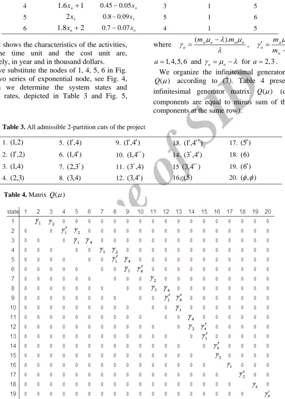
To illustrate the analytical proposed method, we solve a numerical example to present the resource allocation in multi-server dynamic PERT networks, which is presented as the network of queue. It is assumed we have a system with the six service stations depicted as the AoN graph in Fig. 3. We want to determine the optimal resource allocation in multi-server dynamic PERT network for both approaches, namely, resources affecting servers approach and resources as servers approach. For solving this example, we also apply the goal attainment method.
Fig. 3. The AON network of the project under study
4.1. Resources affecting servers
The assumptions of this example for the resources affecting servers approach are:
The new projects, containing all their activities, arrived at the system according to a Poisson process with the rate of 5 per year.
The activity durations (service processing times) are independent random variables with exponential distributions.
The threshold time, u, that project completion time does not exceed is 3 years.
The amount of resources available to be allocated to all service stations is 12.
In all experiments, the value of is equal to 0.01.
Archive of SID
Table 2. Characteristics of the activities
Activity (a) da(xa) ga(xa) ma La Ua 1 2x11 0.60.08x1 4 1 5 2 1.4x2 0.150.01x2 1 1 4 3 1.5x32 0.160.01x3 1 1 4 4 1.6x41 0.450.05x4 3 1 5 5 2x5 0.80.09x5 5 6 1 6 1.8x62 0.70.07x6 4 5 1
Table 2 shows the characteristics of the activities, where the time unit and the cost unit are, respectively, in year and in thousand dollars.
Now, we substitute the nodes of 1, 4, 5, 6 in Fig. 3 with two series of exponential node, see Fig. 4, and then we determine the system states and transition rates, depicted in Table 3 and Fig. 5,
where ( a a ). a a a m m , 1 a a a a m m for 1, 4, 5, 6 a and a a for a2, 3.
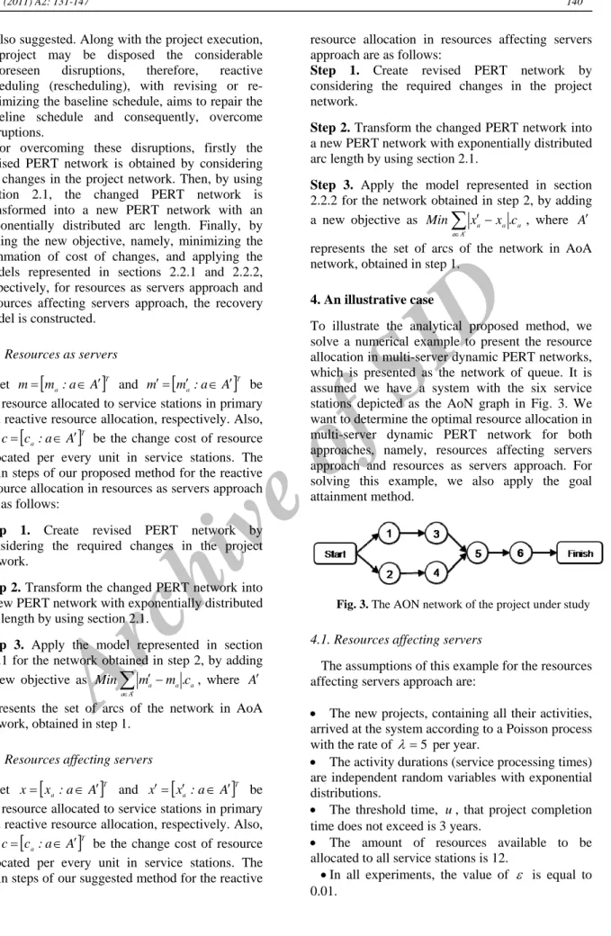
We organize the infinitesimal generator matrix )
(
Q according to (7). Table 4 presents the infinitesimal generator matrix Q() (diagonal components are equal to minus sum of the other components at the same row).
Table 3. All admissible 2-partition cuts of the project
1. (1,2) 5. (1,4) 9. (1,4) 13. (1,4*) 17. (5) 2. (1,2) 6. (1,4) 10. (1,4*) 14. (3*,4) 18. (6) 3. (1,4) 7. (2,3*) 11. (3*,4) 15 (3,4*) 19. (6) 4. (2,3) 8. (3,4) 12. (3,4) 16. (5) 20. (,) Table 4. Matrix Q()
Archive of SID
Table 5. The computational results
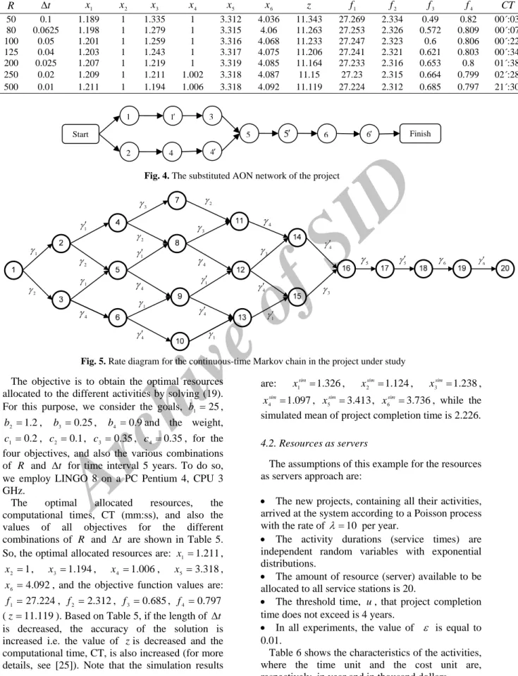
R t x1 x2 x3 x4 x5 x6 z f1 f2 f3 f4 CT 50 0.1 1.189 1 1.335 1 3.312 4.036 11.343 27.269 2.334 0.49 0.82 00´:03˝ 80 0.0625 1.198 1 1.279 1 3.315 4.06 11.263 27.253 2.326 0.572 0.809 00´:07˝ 100 0.05 1.201 1 1.259 1 3.316 4.068 11.233 27.247 2.323 0.6 0.806 00´:22˝ 125 0.04 1.203 1 1.243 1 3.317 4.075 11.206 27.241 2.321 0.621 0.803 00´:34˝ 200 0.025 1.207 1 1.219 1 3.319 4.085 11.164 27.233 2.316 0.653 0.8 01´:38˝ 250 0.02 1.209 1 1.211 1.002 3.318 4.087 11.15 27.23 2.315 0.664 0.799 02´:28˝ 500 0.01 1.211 1 1.194 1.006 3.318 4.092 11.119 27.224 2.312 0.685 0.797 21´:30˝
Fig. 4. The substituted AON network of the project
1 2 1 2 1 4 3 2 1 4 1 4 2 3 4 1 4 1 4 3 4 1 4 3 5 5 6 6
Fig. 5. Rate diagram for the continuous-time Markov chain in the project under study
The objective is to obtain the optimal resources allocated to the different activities by solving (19). For this purpose, we consider the goals, b1 25,
2 . 1
2
b , b3 0.25, b4 0.9and the weight,
2 . 0
1
c , c2 0.1, c3 0.35, c40.35, for the
four objectives, and also the various combinations of R and t for time interval 5 years. To do so, we employ LINGO 8 on a PC Pentium 4, CPU 3 GHz.
The optimal allocated resources, the computational times, CT (mm:ss), and also the values of all objectives for the different combinations of R and t are shown in Table 5. So, the optimal allocated resources are: x1 1.211,
1
2
x , x3 1.194, x4 1.006, x5 3.318,
4.092
6
x , and the objective function values are: 27.224
1
f , f2 2.312, f3 0.685, f4 0.797
(z11.119). Based on Table 5, if the length of t is decreased, the accuracy of the solution is increased i.e. the value of zis decreased and the computational time, CT, is also increased (for more details, see [25]). Note that the simulation results
are: 1 1.326 sim x , 2 1.124 sim x , 3 1.238 sim x , 1.097 4 sim x , 5 3.413 sim x , 6 3.736 sim x , while the simulated mean of project completion time is 2.226.
4.2. Resources as servers
The assumptions of this example for the resources as servers approach are:
The new projects, containing all their activities, arrived at the system according to a Poisson process with the rate of 10 per year.
The activity durations (service times) are independent random variables with exponential distributions.
The amount of resource (server) available to be allocated to all service stations is 20.
The threshold time, u, that project completion time does not exceed is 4 years.
In all experiments, the value of is equal to 0.01.
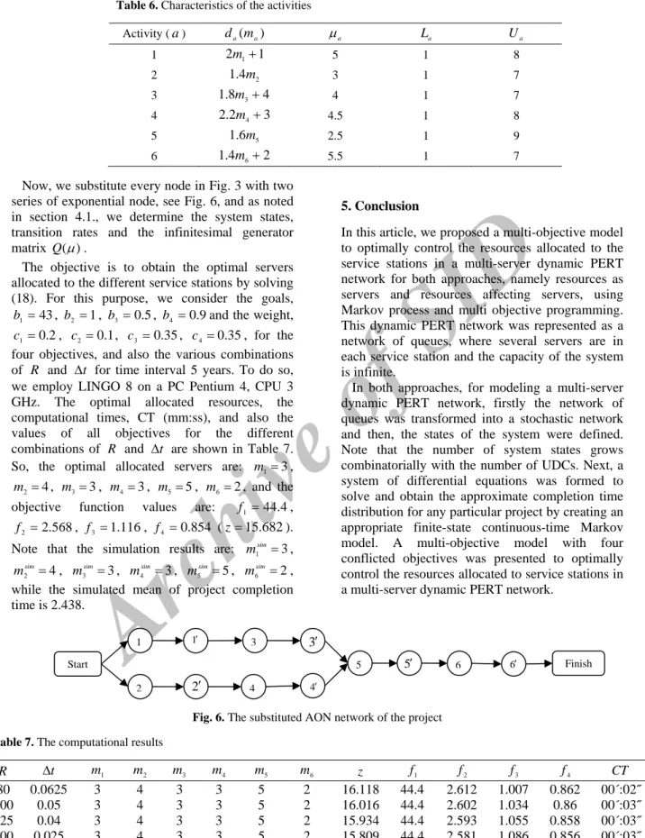
Table 6 shows the characteristics of the activities, where the time unit and the cost unit are, respectively, in year and in thousand dollars.
1 2 5 Start Finish 3 4 1 4 6 5 6
Archive of SID
Table 6. Characteristics of the activities
Activity (a) da(ma) a La Ua 1 2m11 5 1 8 2 1.4m2 3 1 7 3 1.8m34 4 1 7 4 2.2m43 4.5 1 8 5 1.6m5 2.5 9 1 6 1.4m62 5.5 7 1 Now, we substitute every node in Fig. 3 with two
series of exponential node, see Fig. 6, and as noted in section 4.1., we determine the system states, transition rates and the infinitesimal generator matrix Q().
The objective is to obtain the optimal servers allocated to the different service stations by solving (18). For this purpose, we consider the goals,
43
1
b , b2 1, b3 0.5, b4 0.9and the weight,
2 . 0
1
c , c2 0.1, c3 0.35, c40.35, for the
four objectives, and also the various combinations of R and t for time interval 5 years. To do so, we employ LINGO 8 on a PC Pentium 4, CPU 3 GHz. The optimal allocated resources, the computational times, CT (mm:ss), and also the values of all objectives for the different combinations of R and t are shown in Table 7. So, the optimal allocated servers are: m13,
4
2
m , m33, m43, m55, m62, and the
objective function values are: f1 44.4, 568
. 2
2
f , f3 1.116, f4 0.854 (z15.682).
Note that the simulation results are: 1 3
sim m , 4 2 sim m , 3 3 sim m , 4 3 sim m , 5 5 sim m , 6 2 sim m ,
while the simulated mean of project completion time is 2.438.
5. Conclusion
In this article, we proposed a multi-objective model to optimally control the resources allocated to the service stations in a multi-server dynamic PERT network for both approaches, namely resources as servers and resources affecting servers, using Markov process and multi objective programming. This dynamic PERT network was represented as a network of queues, where several servers are in each service station and the capacity of the system is infinite.
In both approaches, for modeling a multi-server dynamic PERT network, firstly the network of queues was transformed into a stochastic network and then, the states of the system were defined. Note that the number of system states grows combinatorially with the number of UDCs. Next, a system of differential equations was formed to solve and obtain the approximate completion time distribution for any particular project by creating an appropriate finite-state continuous-time Markov model. A multi-objective model with four conflicted objectives was presented to optimally control the resources allocated to service stations in a multi-server dynamic PERT network.
Fig. 6. The substituted AON network of the project
Table 7. The computational results
R t m1 m2 m3 m4 m5 m6 z f1 f2 f3 f4 CT 80 0.0625 3 4 3 5 3 2 44.4 16.118 1.0072.612 0.862 00´:02˝ 100 0.05 3 4 3 3 5 16.0162 44.4 2.602 1.034 0.86 00´:03˝ 125 0.04 3 4 3 3 5 15.9342 44.4 2.593 1.055 0.858 00´:03˝ 200 0.025 3 4 3 3 5 15.8092 44.4 2.581 1.086 0.856 00´:03˝ 250 0.02 3 4 3 3 5 15.7672 44.4 1.0962.577 0.855 00´:04˝ 500 0.01 3 4 3 3 5 15.6822 44.4 1.1162.568 0.854 00´:06˝ 1 2 5 Start Finish 3 4 1 4 6 5 6 2 3
Archive of SID
In our model, the total project direct cost wasconsidered as an objective to be minimized and the mean project completion time as another effective objective, should also be accounted to be minimized. The variance of the project completion time was another effective objective in the model, because the mean and the variance are two complementary concepts. The probability that the project completion time does not exceed a certain threshold was considered as the last objective. Finally, the goal attainment method was employed to solve a discrete-time approximation of the primary multi-objective problem.
For obtaining the best optimal allocated resource, we considered the various combinations of portions for a specific time interval. Based on the presented example, if the length of every portion, is decreased, the accuracy of the solution is increased i.e., the value of the objective is decreased and the computational time, CT, is also increased.
Appendix A:
If there is ma server in the service station settled
in the ath node, then the queueing system is
a
m M
M/ / and therefore, the density function of sojourn time (activity duration plus waiting time in queue) is calculated as follow [41]:
( ) (0) ( ) ( ) ( 1) (0) (1 )( ). 0 ( 1) a aa q t a a a a a a a a q m t a a a a a a a a m w w t e m m w m e t m (A-1)
Where and a are, respectively, the arrival
rate of new project and the service rate of service station a. Also, q(0)
a
w , the probability of being zero queue length, and P0 are obtained as follow:
0 ( ) (0) 1 !( ) a m a q a a a a a m w P m m (A-2) and: 1 1 0 1 1 1 ( ) ( ) ( ) ! ! a a m m n a a n a a a a a m P n m m
(A-3) As is observed, obtaining wa(t)in an M/M/mais very hard. We can rewrite the wa(t) as follow, which is similar to two series of exponential distribution with parameters (ma a ) and a:
( ) ( ) (1 (0))( )( ). ( ) (0) (1 ) 0 ( ) aa a m t q a a a a a a a a q t a a a a a a a a a a w t w m e m w m e t m m (A-4)
It seems that we can approximate density function of time spent in service station a with two series exponential. Therefore, our approximate for density function of time spent in service station a would be two series exponential with parameters
( a a ) a m and ( ) (1 ) 1 1 a a a a a a a a m m m , where a a a m
. This approximation is quite simple and easy and there is no need to calculate P0 and
(0)
q a
w which is boring, especially when ma is
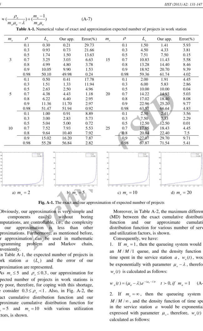
large. Moreover, our approximation can be used in mathematic programming problem and Markov chain, conveniently. We want to evaluate the mean of sojourn time, and therefore, the expected number of projects, and also the cumulative distribution function of sojourn time. In Fig. A-1, the mean number of projects in node a as a changes, is
presented. In the literature, some approximations for the sojourn time in M /M /ma have been
introduced. Sakasegawa [42] proposed closed-form approximation for the expected waiting time in queue, and therefore, the approximation of expected sojourn time W in work station a was calculated as follows: 2( 1) 1 1 1 (1 ) a m a a a a W m (A-5)
Also, Halfin and Whitt [43] developed a closed-form approximation for the q(0)
a
w , and therefore, the approximation of expected sojourn time in work station a was obtained as follows:
2 2 1 1 1 (1 ) 1 2 . ( ). a a a W m e (A-6)
Where (1a) ma and (t) is the
cumulative distribution function of standard normal distribution having mean 0 and variance 1. On the other hand, our approximation for the expected sojourn time in work station a would be:
Archive of SID
1 ( a ) ( a ) a a a a m W m m (A-7)Table A-1. Numerical value of exact and approximation expected number of projects in work station
a
m La Our app. Error(%) ma La Our app. Error(%)
3 0.1 0.30 0.21 29.73 15 0.1 1.50 1.41 5.93 0.3 0.93 0.73 21.66 0.3 4.50 4.33 3.81 0.5 1.74 1.50 13.63 0.5 7.51 7.50 0.15 0.7 3.25 3.03 6.63 0.7 10.83 11.43 5.58 0.8 4.99 4.80 3.78 0.8 13.28 14.40 8.46 0.9 10.05 9.90 1.53 0.9 18.92 20.70 9.39 0.98 50.10 49.98 0.24 0.98 59.36 61.74 4.02 5 0.1 0.50 0.41 17.78 20 0.1 2.00 1.91 4.45 0.3 1.51 1.33 11.94 0.3 6.00 5.83 2.86 0.5 2.63 2.50 4.96 0.5 10.00 10.00 0.04 0.7 4.38 4.43 1.18 0.7 14.22 14.93 5.03 0.8 6.22 6.40 2.95 0.8 17.02 18.40 8.08 0.9 11.36 11.70 2.97 0.9 22.96 25.20 9.77 0.98 51.47 51.94 0.92 0.98 63.57 66.64 4.83 10 0.1 1.00 0.91 8.89 25 0.1 2.50 2.41 3.56 0.3 3.00 2.83 5.73 0.3 7.50 7.33 2.29 0.5 5.04 5.00 0.72 0.5 12.50 12.50 0.01 0.7 7.52 7.93 5.53 0.7 17.65 18.43 4.45 0.8 9.64 10.40 7.92 0.8 20.84 22.40 7.5 0.9 15.02 16.20 7.87 0.9 27.07 29.70 9.71 0.98 55.28 56.84 2.82 0.98 67.87 71.54 5.41 a) ma 2 b) ma 5 c) ma 10 d) ma 20
Fig. A-1. The exact and our approximation of expected number of projects
Obviously, our approximation is very simple and its components easily, without boring computations, are controllable, i.e., the complexity of our approximation is less than other approximations. Furthermore, as mentioned before, our approximation can be used in mathematic programming problem and Markov chain, conveniently.
In Table A-1, the expected number of projects in work station a (La) and the error of our approximation are represented.
As ma5 and a0.3, our approximation for
expected number of projects in work stations is very poor, therefore, for coping with this shortage, we consider 0.3a 1. Also, in Fig. A-2, the exact cumulative distribution function and our approximate cumulative distribution function for
5
a
m and ma10 with various utilization factors, is shown.
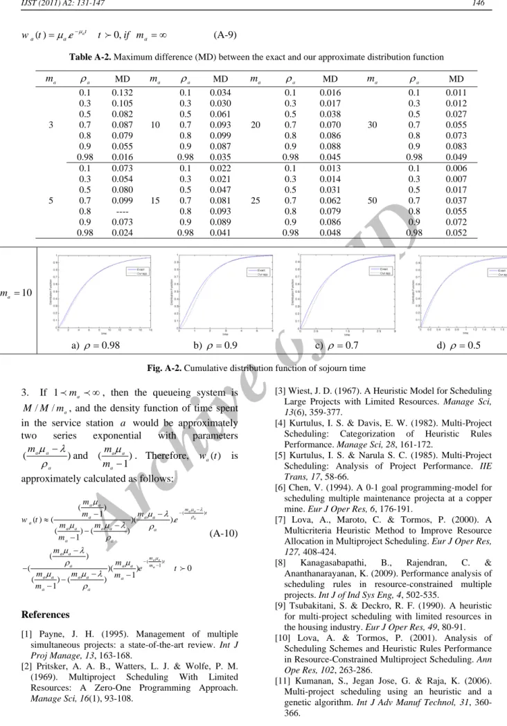
Moreover, in Table A-2, the maximum difference (MD) between the exact cumulative distribution function and our approximate cumulative distribution function for various number of server and utilization factors, is shown.
Consequently, we have:
1. If ma 1, then the queueing system would be an M/M/1 queue, and the density function of time spent in the service station a, wa(t), would be exponentially with parameter a , therefore,
) (t wa is calculated as follows: ( ) ( ) ( ). a t 0, 1 a a a w t e t if m (A-8) 2. If ma , then the queueing system is
/ /M
M , and the density function of time spent in the service station a would be exponentially expressed with parameter a, therefore, wa(t) is
Archive of SID
( ) . at 0,
a a a
w t e t if m (A-9)
Table A-2. Maximum difference (MD) between the exact and our approximate distribution function
a m a MD ma a MD ma a MD ma a MD 3 0.1 0.132 10 0.1 0.034 20 0.1 0.016 30 0.1 0.011 0.3 0.105 0.3 0.030 0.3 0.017 0.3 0.012 0.5 0.082 0.5 0.061 0.5 0.038 0.5 0.027 0.7 0.087 0.7 0.093 0.7 0.070 0.7 0.055 0.8 0.079 0.8 0.099 0.8 0.086 0.8 0.073 0.9 0.055 0.9 0.087 0.9 0.088 0.9 0.083 0.98 0.016 0.98 0.035 0.98 0.045 0.98 0.049 5 0.1 0.073 15 0.1 0.022 25 0.1 0.013 50 0.1 0.006 0.3 0.054 0.3 0.021 0.3 0.014 0.3 0.007 0.5 0.080 0.5 0.047 0.5 0.031 0.5 0.017 0.7 0.099 0.7 0.081 0.7 0.062 0.7 0.037 0.8 ---- 0.8 0.093 0.8 0.079 0.8 0.055 0.9 0.073 0.9 0.089 0.9 0.086 0.9 0.072 0.98 0.024 0.98 0.041 0.98 0.048 0.98 0.052 10 a m a) 0.98 b) 0.9 c) 0.7 d) 0.5
Fig. A-2. Cumulative distribution function of sojourn time
3. If 1ma , then the queueing system is a
m M
M/ / , and the density function of time spent in the service station a would be approximately two series exponential with parameters
) ( a a a m and ) 1 ( a a a m m . Therefore, wa(t) is approximately calculated as follows:
( ) ( ) 1 ( ) 1 ( ) ( )( ). ( ) ( ) 1 ( ) ( )( ) 0 1 ( ) ( ) 1 aa a aa a a a m t a a a a a a a a a a a a a m t m a a a a a a a a a a m m m w t e m m m m m e t m m m m (A-10) References
[1] Payne, J. H. (1995). Management of multiple simultaneous projects: a state-of-the-art review. Int J Proj Manage,13, 163-168.
[2] Pritsker, A. A. B., Watters, L. J. & Wolfe, P. M. (1969). Multiproject Scheduling With Limited Resources: A Zero-One Programming Approach.
Manage Sci,16(1), 93-108.
[3] Wiest, J. D. (1967). A Heuristic Model for Scheduling Large Projects with Limited Resources. Manage Sci, 13(6), 359-377.
[4] Kurtulus, I. S. & Davis, E. W. (1982). Multi-Project Scheduling: Categorization of Heuristic Rules Performance. Manage Sci,28, 161-172.
[5] Kurtulus, I. S. & Narula S. C. (1985). Multi-Project Scheduling: Analysis of Project Performance. IIE Trans,17, 58-66.
[6] Chen, V. (1994). A 0-1 goal programming-model for scheduling multiple maintenance projecta at a copper mine. Eur J Oper Res,6, 176-191.
[7] Lova, A., Maroto, C. & Tormos, P. (2000). A Multicriteria Heuristic Method to Improve Resource Allocation in Multiproject Scheduling. Eur J Oper Res, 127, 408-424.
[8] Kanagasabapathi, B., Rajendran, C. & Ananthanarayanan, K. (2009). Performance analysis of scheduling rules in resource-constrained multiple projects. Int J of Ind Sys Eng,4, 502-535.
[9] Tsubakitani, S. & Deckro, R. F. (1990). A heuristic for multi-project scheduling with limited resources in the housing industry. Eur J Oper Res,49, 80-91. [10] Lova, A. & Tormos, P. (2001). Analysis of
Scheduling Schemes and Heuristic Rules Performance in Resource-Constrained Multiproject Scheduling. Ann Ope Res,102, 263-286.
[11] Kumanan, S., Jegan Jose, G. & Raja, K. (2006). Multi-project scheduling using an heuristic and a genetic algorithm. Int J Adv Manuf Technol,31, 360-366.
Archive of SID
[12] Gonçalves, J. F., Mendes, J. J. M. & Resende, M. G. C. (2008). A genetic algorithm for the resource constrained multi-project scheduling problem. Eur J Oper Res,189, 1171-1190.
[13] Ying, Y., Shou, Y. & Li, M. (2009). Hybrid genetic algorithm for resource constrained multi-project scheduling problem. J Zhejiang Uni (Eng Sci),43, 23-27.
[14] Chen, P. H. & Shahandashti, S. M. (2009). Hybrid of genetic algorithm and simulated annealing for multiple project scheduling with multiple resource constraints.
Autom Constr,18, 434-443.
[15] Kruger, D. & Scholl, A. (2008). Managing and modelling general resource transfers in (multi-) project scheduling. OR Spectrum,32, 369-394.
[16] Fatemi-Ghomi, S. M. T. & Ashjari B. (2002). A simulation model for multi-project resource allocation.
Int J Proj Manage,20, 127-130.
[17] Nozick, L. K., Turnquist, M. A. & Xu, N. (2004). Managing portfolios of projects under uncertainty. Ann Ope Res,132, 243-256.
[18] Kao, H. P., Hsieh, B. & Yeh, Y. (2006). A petri-net based approach for scheduling and rescheduling resource-constrained multiple projects. J Chin Inst Ind Eng,23(6), 468-477.
[19] Byali, R. P. & Kannan, M. V (2008). Critical Chain Project Management-A new project management philosophy for multi project environment. J Spacecraft Tech, 18, 30-36.
[20] Adler, P. S., Mandelbaum, A., Nguyen, V. & Schwerer, E. (1995). From project to process management: an empirically-based framework for analyzing product development time. Manage Sci,
41(3), 458-484.
[21] Anavi-Isakow, S. & Golany, B. (2003). Managing multi-project environments hrough constant work-in-process. Int J Proj Manage, 21(1), 9-18.
[22] Li, C. & Wang, K. (2009). The risk element transmission theory research of multi-objective risk-time-cost trade-of. Comput Math Appl 57, 1792–1799. [23] Cohen, I., Golany, B. & Shtub, A. (2005). Managing
stochastic, finite capacity, multi-project systems through the Cross Entropy methodology. Ann Ope Res,
134, 183-199.
[24] Cohen, I., Golany, B. & Shtub, A. (2007). Resource allocation in stochastic, finite-capacity, multi-project systems through the cross entropy methodology. J Sched, 10, 181-193.
[25] Azaron, A. & Tavakkoli-Moghaddam, R. (2007). Multi-objective time–cost trade-off in dynamic PERT networks using an interactive approach. Eur J Oper Res, 180, 1186-1200.
[26] Yaghoubi, S., Noori, S., Azaron, A. & Tavakkoli-Moghaddam, R. (2011). Resource allocation in dynamic PERT networks with finite capacity. Eur J Oper Res, 215,670-678.
[27] Szelke, E. & Kerr, R.M. (1994). Knowledge-based reactive scheduling. Prod Plan Con,5(2), 124-145. [28] Sabuncuoglu, I. & Bayiz, M. (2000). Analysis of
reactive scheduling problems in a job shop environment. Eur J Oper Res,126, 567-586.
[29] Vieira, G. E., Herrmann, J. W. & Lin, E. (2003). Rescheduling manufacturing systems: A framework of strategies, policies and methods. J Sched 6, 39-62. [30] Aytug, H., Lawley, M. A., McKay, K., Mohan, S. &
Uzsoy, R. (2005). Executing production schedules in the face of uncertainties: A review and some future directions. Eur J Oper Res, 161(1), 86-110.
[31] Herroelen, W. & Leus, R. (2005). Project scheduling under uncertainty-Survey and research potentials. Eur J Oper Res,165, 289-306.
[32] Van de Vonder, S., Demeulemeester, E. & Herroelen, W. (2007). A classification of predicti