Machine Learning for Internet of Things Data Analysis:
A Survey
Mohammad Saeid Mahdavinejad1, Mohammadreza Rezvan2, Mohammadamin Barekatain3, Peyman Adibi4, Payam Barnaghi5, Amit P. Sheth6
Abstract
Rapid developments in hardware, software, and communication technologies have allowed the emergence of Internet-connected sensory devices that provide observation and data measurement from the physical world. By 2020, it is estimated that the total number of Internet-connected devices being used will be between 25-50 billion. As the numbers grow and technologies become more mature, the volume of data published will increase. Internet-connected devices technology, referred to as Internet of Things (IoT), continues to extend the current Internet by providing connectivity and interaction between the physical and cyber worlds. In addition to increased volume, the IoT generates Big Data characterized by velocity in terms of time and location dependency, with a variety of multiple modalities and varying data quality. Intelligent processing and analysis of this Big Data is the key to developing smart IoT applications. This article assesses the different machine learning methods that deal with the challenges in IoT data by considering smart cities as the main use case. The key contribution of this study is presentation of a taxonomy of machine learning algorithms explaining how different techniques are applied to the data in order to extract higher level information. The potential and challenges of machine
∗Corresponding author
Email address: [email protected](Payam Barnaghi) 1University of Isfahan, Kno.e.sis - Wright State University 2University of Isfahan, Kno.e.sis - Wright State University 3Technische Universit¨at M¨unchen
4University of Isfahan 5University of Surrey
learning for IoT data analytics will also be discussed. A use case of applying Support Vector Machine (SVM) on Aarhus Smart City traffic data is presented for a more detailed exploration.
Keywords: Machine Learning, Internet of Things, Smart Data, Smart City
1. Introduction
Emerging technologies in recent years and major enhancements to Internet protocols and computing systems, have made the communication between dif-ferent devices easier than ever before. According to various forecasts, around 25-50 billion devices are expected to be connected to the Internet by 2020. This 5
has given rise to the newly developed concept of Internet of Things (IoT). IoT is a combination of embedded technologies regarding wired and wireless com-munications, sensor and actuator devices, and the physical objects connected to the Internet [1, 2]. One of the long-standing objectives of computing is to simplify and enrich human activities and experiences (e.g., see the visions asso-10
ciated with “The Computer for the 21st Century” [3] or “Computing for Human Experience” [4]) IoT needs data to either represent better services to users or enhance IoT framework performance to accomplish this intelligently. In this manner, systems should be able to access raw data from different resources over the network and analyze this information to extract knowledge.
15
Since IoT will be among the greatest sources of new data, data science will make a great contribution to make IoT applications more intelligent. Data sci-ence is the combination of different fields of scisci-ences that uses data mining, machine learning and other techniques to find patterns and new insights from data. These techniques include a broad range of algorithms applicable in differ-20
ent domains. The process of applying data analytics methods to particular areas involves defining data types such as volume, variety, velocity; data models such as neural networks, classification, clustering methods and applying efficient al-gorithms that match with the data characteristics. By following our reviews, it is deduced that: firstly, since data is generated from different sources with spe-25
cific data types, it is important to adopt or develop algorithms that can handle the data characteristics, secondly, the great number of resources that generate data in real time are not without the problem of scale and velocity and thirdly, finding the best data model that fits the data is one of the most important issues for pattern recognition and for better analysis of IoT data. These issues 30
have opened a vast number of opportunities in expanding new developments. Big Data is defined as high-volume, high-velocity, and high variety data that demand cost-effective, innovative forms of information processing which enable enhanced insight, decision making, and process automation[5].
With respect to the challenges posed by Big Data, it is necessary to divert 35
to a new concept termed Smart Data, which means: ”realizing productivity, efficiency, and effectiveness gains by using semantics to transform raw data into Smart Data” [6] . A more recent definition of this concept is: ”Smart Data pro-vides value from harnessing the challenges posed by volume, velocity, variety, and veracity of Big Data, and in turn providing actionable information and im-40
proving decision making.” [7]. At last, Smart Data can be a good representative for IoT data.
1.1. The Contribution of this paper
The objective here is to answer the following questions:
A)How could machine learning algorithms be applied to IoT smart
45
data?
B)What is the taxonomy of machine learning algorithms that can
be adopted in IoT?
C)What are IoT data characteristics in real-world?
D)Why is the Smart City a typical use case of IoT applications?
50
A) To understand which algorithm is more appropriate for processing and decision-making on generated smart data from the things in IoT, realizing these three concepts is essential. First, the IoT application (Sec. 3), second, the IoT data characteristics (Sec, 4.2), and the third, the data-driven vision of machine learning algorithms (Sec. 5). We finally discussed the issues in Sec. 6.
B) About 70 articles in the field of IoT data analysis are reviewed, revealing that there exist eight major groups of algorithms applicable to IoT data. These algorithms are categorized according to their structural similarities, type of data they can handle, and the amount of data they can process in reasonable time.
C) Having reviewed the real-work perspective of how IoT data is analyzed 60
by over 20 authors, many significant and insightful results have been revealed regarding data characteristics. We discussed the results in Sec. 6 and Table 1. To have a deeper insight into IoT smart data, patterns must be extracted and the generated data interpreted. Cognitive algorithms will undertake interpretation and matching, much as the human mind would do. Cognitive IoT systems will 65
learn from the data previously generated and will improve when performing repeated tasks. Cognitive computing as as a prosthetic for human cognition by analyzing massive amounts of data and being able to respond to questions humans might have when making certain decisions. Cognitive Iot plays an important role in enabling the extraction of meaningful patterns form the IoT 70
smart data generated [8].
D) Smart City has been selected as our primary use case in IoT for three reasons: Firstly, among all of the reviewed articles the focus of 60 percents is on the field of the Smart City, secondly, Smart City includes many of the other use cases in IoT, and thirdly, there are many open datasets for Smart City 75
applications easily accessible for researchers. Also, Support Vector Machine (SVM) algorithm is implemented on the Aarhus City smart traffic data in order to predict traffic hours during one day in Sec. 6. By answering the above questions about the IoT smart data and machine learning algorithms, we would be able to choose the best machine learning algorithm that can handle IoT 80
smart data characteristics. Unlike the others, similar surveys about the machine learning and IoT, readers of this article would be able to get deep and technical understanding of machine learning algorithms, IoT applications, and IoT data characteristics along with both technical and simple implementations.
Figure 1: Organization of survey
1.2. Organization 85
The rest of this paper is organized as follows: the related articles in this field are reviewed and reported in Sec. 2. IoT applications and communication protocols, computing frameworks, IoT architecture, and Smart City segments are reviewed, explained, briefed and illustrated in Sec. 3. The quality of data, Big Data generation, integrating sensor data and semantic data annotation are 90
reviewed in Sec. 4. Machine learning algorithms in eight categories based on recent researches on IoT data and frequency of machine learning algorithms are reviewed and briefed in Sec. 5. Matching the algorithms to the particular Smart City applications is done in Sec. 6, and the conclusion together with future research trends and open issues are presented in Sec. 7.
95
2. Literature Review
Since IoT represents a new concept for the Internet and smart data, it is a challenging area in the field of computer science. The important challenges for researchers with respect to IoT consist of preparing and processing data.
[9] proposed 4 data mining models for processing IoT data. The first pro-100
posed model is a multi layer model, based on a data collection layer, a data management layer, an event processing model, and data mining service layer. The second model is adistributed data mining model, proposed for data deposi-tion at different sites. The third model is agrid based data mining model where the authors seek to implement heterogeneous, large scale and high performance 105
applications, and the last model is adata mining model from multi technology integration perspective, where the corresponding framework for a future Internet is described.
[10] performed research into warehousing radio frequency identification, (RFID) data, with a focus on managing and mining RFID stream data, specifically. 110
[11] introduce a systematic manner for reviewing data mining knowledge and techniques in most common applications. In this study, they reviewed some data mining functions like classification, clustering, association analysis, time series analysis, and outline detection. They revealed that the data generated by data mining applications such as e-commerce, Industry, healthcare, and city gover-115
nance are similar to that of the IoT data. Following their findings, they assigned the most popular data mining functionality to the application and determined which data mining functionality was the most appropriate for processing each specific application’s data.
[12] ran a survey to respond to some of the challenges in preparing and 120
processing data on the IoT through data mining techniques. They divided their research into three major sections, in the first and second sections; they explain IoT, the data, and the challenges that exist in this area, such as building a model of mining and mining algorithms for IoT. In the third section, they discuss the potential and open issues that exist in this field. Then, data mining on IoT 125
data have three major concerns: first, it must be shown that processing data will solve the chosen problems. Next the data characteristics must be extracted from generated data, and then, the appropriate algorithm is chosen according to the taxonomy of algorithms and data characteristics.
[13] attempted to explain the Smart City infrastructure in IoT and discussed 130
the advanced communication to support added-value services for the adminis-tration of the city and citizens thereof. They provide a comprehensive view of enabling technologies, protocols, and architectures for Smart City. In the technical part of their, the article authors reviewed the data of Padova Smart City.
135
3. Internet of Things
The purpose of Internet of Things, (IoT) is to develop a smarter environ-ment, and a simplified life-style by saving time, energy, and money. Through this technology, the expenses in different industries can be reduced. The enor-mous investments and many studies running on IoT has made IoT a growing 140
trend in recent years. IoT is a set of connected devices that can transfer data among one another in order to optimize their performance; these actions occur automatically and without human awareness or input. IoT includes four main components: 1) sensors, 2)processing networks, 3) analyzing data, and 4) mon-itoring the system. The most recent advances made in IoT began when radio 145
frequency identification (RFID) tags were put into use more frequently, lower cost sensors became more available, web technology developed, and communica-tion protocols changed [14, 15]. The IoT is integrated with different technologies and connectivity is necessary and sufficient condition for it. So communication protocols are constituents the technology that should be enhanced [16, 17]. In 150
IoT, communication protocols can be divided into three major components: (1) Device to Device (D2D): this type of communication enables communi-cation between nearby mobile phones. This is the next generation of cellular networks.
(2) Device to Server (D2S): in this type of communication devices, all the 155
data is sent to the servers, which can be close or far from the devices. This type of communication mostly is applied in cloud processing.
data between each other. This type of communication mostly is applied in cellular networks.
160
Processing and preparing data for these communications is a critical chal-lenge. To respond to this challenge, different kinds of data processing, such as analytics at the edge, stream analysis, and IoT analysis at the database, must be applied. The decision to apply any one of the mentioned processes depends on the particular application and its needs[18]. Fog and cloud processing are two 165
analytical methods adopted in processing and preparing data before transfer-ring to the other things. The whole task of IoT is summarized as follows: first, sensors and IoT devices collect the information from the environment. Next, knowledge should be extracted from the raw data. Then, the data will be ready for transfer to other objects, devices, or servers through the Internet.
170
3.1. Computing Framework
Another important part of IoT iscomputing frameworksfor processing data, the most famous of which are fog and cloud computing. IoT applications use both frameworks depending on application and process location. In some appli-cations, data should be processed upon generation, while in other appliappli-cations, 175
it is not necessary to process data immediately. The instant processing of data and the network architecture that supports it is known as fog computing. Col-lectively, they are applied for edge computing[19].
3.1.1. Fog Computing:
Here, the architecture of fog computing is applied to migrate information 180
from the data centers task to the edge of the servers. This architecture is built based on the edge servers. Fog computing provides limited computing, storage, and network services, also providing logical intelligence and filtering of data for data centers. This architecture has been and is being implemented in vital areas like eHealth and military applications [20, 21].
3.1.2. Edge Computing:
In this architecture, processing is run at a distance from the core, toward the edge of the network. This type of processing enables data to be initially processed at the edge devices. Devices at the edge may not be connected to the network in a continuous manner, so they need a copy of master data/reference 190
data for offline processing. Edge devices have different features such as 1)en-hancing security, 2)filtering and cleaning of the data, and 3)storing local data for local use[22].
3.1.3. Cloud Computing:
Here, data for processing is sent to the data centers, and after being analyzed 195
and processed, they become accessible.
This architecture has high latency and high load balancing, indicating that this architecture is not sufficient enough for processing IoT data because most processing should run at high speeds. The volume of this data is high, and Big Data processing will increase the CPU usage of the cloud servers[23]. There are 200
different types of cloud computing:
(1)Infrastructure as a Service (IaaS): where the company purchases all the equipment like hardware, servers , and networks.
(2) Platform as a Service (PaaS): where all the equipment above, are put for rent on the Internet.
205
(3) Software as a service(SaaS): where a distributed software model is pre-sented. In this model, all the practical software will be hosted from a service provider, and practical software can be accessible to the users through the In-ternet [24].
(4) Mobile Backend as a Service (MBaaS): also known as a Backend as a 210
Service(BaaS), provides the web and mobile application with a path in order to connect the application to the backend cloud storage. MBaaS provides features like user management, push notification and integrates with the social network services. This cloud service benefits from application programming interface (API) and software development kits (SDK).
3.1.4. Distributed Computing
: This architecture is designed for processing high volume data. In IoT applications, because the sensors generate data on a repeated manner, Big Data challenges are encountered[22, 25]. To overcome this phenomenon, a distributed computing is designed to divide data into packets, and assign each packet to 220
different computers for processing. This distributed computing has different frameworks like Hadoop and Spark. When migrating from cloud to fog and distributed computing, the following occur: 1) a decrease in network loading, 2) an increase in data processing speed, 3) a reduction in CPU usage, 4) a reduction in energy consumption, and 5) higher data volume processing. 225
Because the Smart City is one of the primary applications of IoT, the most important use cases of Smart City and their data characteristics are discussed in the following sections.
4. Smart City
Cities always demand services to enhance the quality of life and make ser-230
vices more efficient. In the last few years, the concept of smart cities has played an important role in academia and in industry [26]. With an increase in the population and complexity of city infrastructures, cities seek manners to handle large-scale urbanization problems. IoT plays a vital role in collecting data from the city environment. IoT enables cities to use live status reports and smart 235
monitoring systems to react more intelligently against the emerging situations such as earthquake and volcano. By using IoT technologies in cities, the ma-jority of the city’s assets can be connected to one another, make them more readily observable, and consequently, more easy to monitor and manage. The purpose of building smart cities is to improve services like traffic management, 240
water management, and energy consumption, as well as improving the quality of life for the citizens. The objectives of smart cities is to transform rural and urban areas into places of democratic innovation [27]. Such smart cities seek to decrease the expenses in public health, safety, transportation and resource
management, thus assisting the their economy [28]. 245
[29] Believe that in the long term, the vision for a Smart City would be that all the cities’ systems and structures will monitor their own conditions and carry out self-repair upon need.
4.1. Use Case
A city has an important effect on society because the city touches all aspects 250
of human life. Having a Smart City can assist in having a comfortable life. Smart Cities use cases consist of Smart Energy, smart mobility, Smart Citizens, and urban planning. This division is based on reviewing the latest studies in this field and the most recent reports released by McKinsey and Company.
4.1.1. Smart Energy 255
Smart Energy is one of the most important research areas of IoT because it is essential to reduce overall power consumption[30]. It offers high-quality, affordable environment energy friendly. Smart Energy includes a variety of op-erational and energy measures, including Smart Energy applications, smart leak monitoring, renewable energy resources, etc. Using Smart Energy(i.e., deploy-260
ment of a smart grid) implies a fundamental re-engineering of the electricity services[31]. Smart Grid is one of the most important applications of Smart Energy. It includes many high-speed time series data to monitor key devices. For managing this kind of data, [32] have introduced a method to manage and analyze time series data in order to make them organized on demand. Moreover, 265
Smart Energy infrastructure will become more complex in future, therefore [33] have proposed a simulation system to test new concept and optimization ap-proaches and forecast future consumption. Another important application of Smart Energy is a leak monitoring system. The objective of this system is to model a water or gas management system which would optimize energy resource 270
4.1.2. Smart Mobility
Mobility is another important part of the city. Through the IoT, city officials can improve the quality of life in the city. Smart mobility can be divided into the following three major parts:
275
(1) Autonomous cars: IoT will have a broad range effect on how vehicles are run. The most important question is about how IoT can improve vehicle services. IoT sensors and wireless connections make it possible to create self-driving cars and monitor vehicles performance. With the data collected from vehicles, the most popular/congested routes can be predicted, and decisions can 280
be made to decrease the traffic congestion. Self-driving cars can improve the passenger safely because they have the ability to monitor the driving of other cars.
(2) Traffic control: Optimizing the traffic flow by analyzing sensor data is another part of mobility in the city. In traffic control, traffic data will be 285
collected from the cars, road cameras, and from counter sensors installed on roads.
(3)Public transportation: IoT can improve the public transportation system management by providing accurate location and routing information to smart transportation system. It can assist the passengers in making better decisions 290
in their schedules as well as decrease the amount of wasted time. There exist different perspectives over how to build smart public transportation systems. These systems need to manage a different kind of data like vehicle location data and traffic data. Smart public transportation systems should be real-time oriented in order to make proper decisions in real-time as well as use historical 295
data analysis [36]. For instance, [37] have proposed a mechanism that considers Smart City devices as graph nodes and they have used Big Data solutions to solve these issues.
4.1.3. Smart Citizen
This use case for Smart Cities covers a broad range of areas in human lives, 300
envi-ronment with all its components is fundamental and vital for life; consequently, making progress in technology is guaranteed to enhance security. Close moni-toring devoted to crime would also contribute to overall social health .
4.1.4. Urban Planning 305
Another important aspect in use cases for the Smart City is drawing long-term decisions. Since the city and environment have two major roles in human life, drawing decisions in this context is critical. By collecting data from different sources, it is possible to draw a decision for the future of the city. Drawing decisions affecting the city infrastructure, design, and functionality is called 310
urban planning. IoT is beneficial in this area because through Smart City data analysis, the authorities can predict which part of the city will be more crowded in the future and find solutions for the potential problems. A combination of IoT and urban planning would have a major affect on scheduling future infrastructure improvements.
315
4.2. Smart City Data Characteristics
Smart cities’ devices generate data on a continuous manner, indicating that the data gathered from traffic, health, and energy management applications would provide sizable volume. In addition, since the data generation rate varies for different devices, processing data with different generation rates is a chal-320
lenge. For example, frequency of GPS sensors updating is measured in sec-onds while, the frequency of updates for temperature sensors may be measured hourly. Whether the data generation rate is high or low, there always exists the danger of important information loss. To integrate the sensory data collected from heterogeneous sources is challenging[14, 38]. [39] applied Big Data analytic 325
methods to distinguish the correlation between the temperature and traffic data in Santander City, Spain.
[40] proposed a new framework integrating Big Data analysis and Industrial Internet of Things (IIoT) technologies for Offshore Support Vessels (OSV) based on a hybrid CPU/GPU high-performance computing platform.
Another characteristic is the dynamic nature of the data. Autonomous cars’ data is an example of Dynamic Data because the sensor results will change based on different locations and times.
The quality of the collected data is important, particularly the Smart City data which have different qualities due to the fact that they are generated from 335
heterogeneous sources. According to[41], the quality of information from each data source depends on three factors:
1) Error in measurements or precision of data collection. 2) Devices’ noise in the environment.
3) Discrete observation and measurements. 340
To have a better Quality of Information (QoI), it is necessary to extract higher levels of abstraction and provide actionable information to other ser-vices. QoI in Smart Data depends on the applications and characteristics of data. There exist different solutions to improve QoI. For example, to improve the accuracy of data, selecting trustworthy sources and combining the data 345
from multiple resources is of essence. By increasing frequency and density of sampling, precision of the observations and measurements will be improved, which would lead a reduction in environmental noise. The data characteristics in both IoT and Smart City are shown in Figure 2. Semantic data annotation is another prime solution to enhance data quality. Smart devices generate raw 350
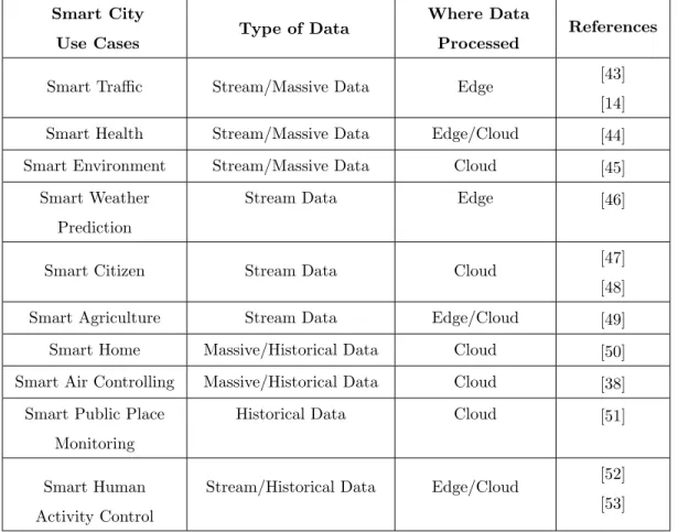
data with low-level abstractions; for this reason, the semantic models will pro-vide interpretable descriptions on data, its quality, and original attributes [28]. Semantic annotation is beneficial in interpretable and knowledge-based infor-mation fusion[42]. Smart data characteristics in smart cities are tabulated in brief, in Table 1.
355
5. Taxonomy of machine learning algorithms
Machine learning is a sub field of computer science, a type of Artificial Intel-ligence, (AI), that provides machines with the ability to learn without explicit programming. Machine learning evolved from pattern recognition and
Compu-Table 1: Characteristic of Smart Data in smart cities
Smart City
Use Cases Type of Data
Where Data Processed
References
Smart Traffic Stream/Massive Data Edge [43]
[14]
Smart Health Stream/Massive Data Edge/Cloud [44]
Smart Environment Stream/Massive Data Cloud [45]
Smart Weather Prediction
Stream Data Edge [46]
Smart Citizen Stream Data Cloud [47]
[48]
Smart Agriculture Stream Data Edge/Cloud [49]
Smart Home Massive/Historical Data Cloud [50]
Smart Air Controlling Massive/Historical Data Cloud [38]
Smart Public Place Monitoring
Historical Data Cloud [51]
Smart Human Activity Control
Stream/Historical Data Edge/Cloud [52]
IoT Dat a Cha ra ct e ris tic s Big Data Volume Variety Velocity Data Quality Redundancy Accuracy Dynamicity Granularity Data Usage Semantic Completeness Noiseless
Figure 2: Data characteristics
tational Learning Theory. There, some essential concepts of machine learning 360
are discussed as well as, the frequently applied machine learning algorithms for smart data analysis.
A learning algorithm takes a set of samples as an input named a training set. In general, there exist three main categories of learning: supervised, un-supervised, and reinforcement [54, 55, 56]. In an informal sense, in supervised 365
learning, the training set consists of samples of input vectors together with their corresponding appropriate target vectors, also known aslabels. In unsupervised learning, no labels are required for the training set. Reinforcement learning deals with the problem of learning the appropriate action or sequence of actions to be taken for a given situation in order to maximize payoff. This article focuses 370
is on supervised and unsupervised learning since they have been and are being widely applied in IoT smart data analysis. The objective of supervised learning is to learn how to predict the appropriate output vector for a given input vector. Applications where the target label is a finite number of discrete categories are
known asclassification tasks. Cases where the target label is composed of one 375
or more continuous variables are known asregression [57].
Defining the objective of unsupervised learning is difficult. One of the major objectives is to identify the sensible clusters of similar samples within the input data, known asclustering. Moreover, the objective may be the discovery of a useful internal representation for the input data by preprocessing the original 380
input variable in order to transfer it into a new variable space. This preprocess-ing stage can significantly improve the result of the subsequent machine learnpreprocess-ing algorithm and is namedfeature extraction [55].
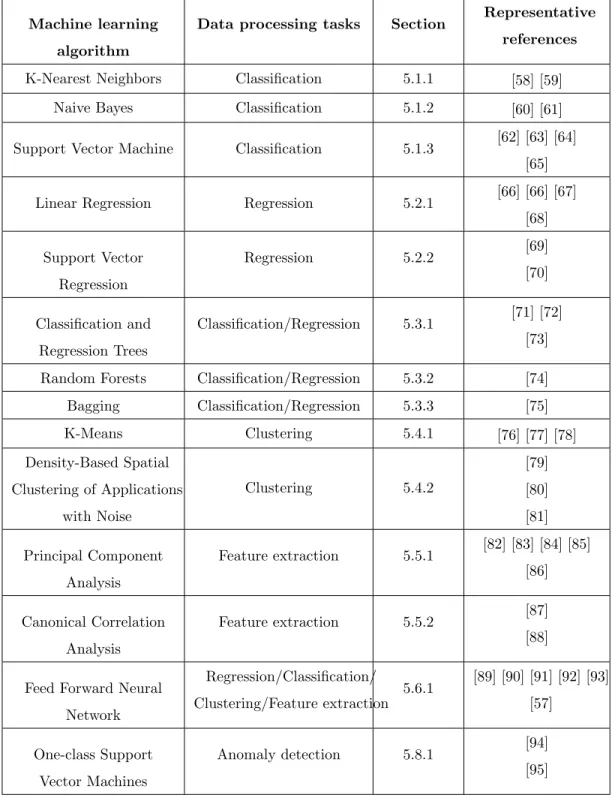
The frequently applied machine learning algorithms for smart data analysis are tabulated in Table 2.
385
In the following subsections, we assume that we are given a training set containing N training samples denoted as {(xi, yi)}Ni=1, where xi is the the
ith training M-dimensional input vector and y
i is it’s corresponding desired
P-dimensional output vector. Moreover, we collect the M-dimensional input vectors into a matrix, written x ≡ (x1, . . . , xN)T, and we also collect their
390
corresponding desired output vectors in a matrix, written y ≡ (y1, . . . , yN)T.
However, in Section 5.4 the training set does not contain the desired output vectors.
5.1. Classification
5.1.1. K-Nearest Neighbors 395
In K-nearest neighbors (“KNN”), the objective is to classify a given new, unseen data point by looking atK given data points in the training set, which are closest in input or feature space. Therefore, in order to find theK nearest neighbors of the new data point, we have to use a distance metric such as Eu-clidean distance,L∞ norm, angle, Mahalanobis distance or Hamming distance.
400
To formulate the problem, let us denote the new input vector (data point) by x, it’sK nearest neighbors by Nk(x), the predicted class label for xbyy, and
the class variable by a discrete random variable t. Additionally, 1(.) denotes indicator function: 1(s) = 1 if sis true and 1(s) = 0 otherwise. The form of
Table 2: Overview of frequently used machine learning algorithms for smart data analysis
Machine learning algorithm
Data processing tasks Section Representative
references
K-Nearest Neighbors Classification 5.1.1 [58] [59]
Naive Bayes Classification 5.1.2 [60] [61]
Support Vector Machine Classification 5.1.3 [62] [63] [64]
[65]
Linear Regression Regression 5.2.1 [66] [66] [67]
[68] Support Vector Regression Regression 5.2.2 [69] [70] Classification and Regression Trees Classification/Regression 5.3.1 [71] [72] [73]
Random Forests Classification/Regression 5.3.2 [74]
Bagging Classification/Regression 5.3.3 [75] K-Means Clustering 5.4.1 [76] [77] [78] Density-Based Spatial Clustering of Applications with Noise Clustering 5.4.2 [79] [80] [81] Principal Component Analysis Feature extraction 5.5.1 [82] [83] [84] [85] [86] Canonical Correlation Analysis Feature extraction 5.5.2 [87] [88]
Feed Forward Neural Network Regression/Classification/ Clustering/Feature extraction 5.6.1 [89] [90] [91] [92] [93] [57] One-class Support Vector Machines Anomaly detection 5.8.1 [94] [95]
the classification task is 405 p(t=c|x, K) = 1 K X i∈Nk(x) 1(ti=c), y= arg max c p(t=c|x, K) (1)
i.e., the input vectorxwill be labeled by the mode of its neighbors’ labels [58].
One limitation of KNN is that it requires storing the entire training set, which makes KNN unable to scale large data sets. In [59], authors have ad-dressed this issue by constructing a tree-based search with some one-off com-410
putation. Moreover, there exists an online version of KNN calcification. It is worth noting that KNN can also be used for regression task [55]. However we don’t explain it here, since it is not a frequently used algorithm for smart data analysis. [96] proposes a new framework for learning a combination of multiple metrics for a robust KNN classifier. Also, [47] compares K-Nearest Neighbor 415
with a rough-set-based algorithm for classifying the travel pattern regularities.
5.1.2. Naive Bayes
Given a new, unseen data point (input vector)z= (z1, . . . , zM), naive Bayes
classifiers, which are a family of probabilistic classifiers, classify z based on applying Bayes’ theorem with the “naive” assumption of independence between the features (attributes) ofz given the class variablet. By applying the Bayes’ theorem we have
p(t=c|z1, . . . , zM) =
p(z1, . . . , zM|t=c)p(t=c)
p(z1, . . . , zM)
(2) and by applying the naive independence assumption and some simplifications we have p(t=c|z1, . . . , zM)∝p(t=c) M Y j=1 p(zj|t=c) (3)
Therefore, the form of the classification task is
y= arg max c p(t=c) M Y j=1 p(zj|t=c) (4)
where y denotes the predicted class label for z. The different naive Bayes classifiers use different approaches and distributions to estimate p(t = c) and p(zj|t=c) [61].
420
Naive Bayes classifiers require a small number of data points to be trained, can deal with high-dimensional data points, and are fast and highly scalable [60]. Moreover, they are a popular model for applications such as spam filtering [97], text categorization, and automatic medical diagnosis [98]. [49] used this 425
algorithm to combine factors to evaluate the trust value and calculate the final quantitative trust of the Agricultural product.
5.1.3. Support Vector Machine
The classical Support Vector Machines (SVMs) are non-probabilistic, bi-nary classifiers that aim at finding the dividing hyperplane which separates both classes of the training set with the maximum margin. Then, the predicted label of a new, unseen data point, is determined based on which side of the hy-perplane it falls [62]. First, we discuss the Linear SVM that finds a hyhy-perplane, which is a linear function of the input variable. To formulate the problem, we denote the normal vector to the hyperplane bywand the parameter for control-ling the offset of the hyperplane from the origin along its normal vector by b. Moreover, in order to ensure that SVMs can deal with outliers in the data, we introduce variableξi, that is, a slack variable, for every training pointxi that
gives the distance of how far this training point violates the margin in the units of |w|. This binary linear classification task is described using a constrained optimization problem of the form
minimize w,b,ξ f(w, b, ξ) = 1 2w Tw+C n X i=1 ξi subject to yi(wTxi+b)−1 +ξi ≥0 i= 1, . . . , n, ξi≥0 i= 1, . . . , n. (5)
where parameterC >0 determines how heavily a violation is punished [65, 63]. It should be noted that although here we used L1 norm for the penalty term
Pn
i=1ξi, there exist other penalty terms such asL2norm which should be
cho-sen with respect to the needs of the application. Moreover, parameterC is a hyperparameter which can be chosen via cross-validation or Bayesian optimiza-tion. To solve the constrained optimization problem of equation 5, there are various techniques such as quadratic programming optimization [99], sequential 435
minimal optimization [100], and P-packSVM [101]. One important property of SVMs is that the resulting classifier only uses a few training points, which are calledsupport vectors, to classify a new data point.
In addition to performing linear classification, SVMs can perform a non-linear classification which finds a hyperplane that is a non-linear function of the input 440
variable. To do so, we implicitly map an input variable into high-dimensional feature spaces, a process which is calledkernel trick [64]. In addition to per-forming binary classification, SVMs can perform multiclass classification. There are various ways to do so, such as One-vs-all (OVA) SVM, All-vs-all (AVA) SVM [54], Structured SVM [102], and the Weston and Watkins [103] version. 445
SVMs are among the best off-the-shelf, supervised learning models that are capable of effectively dealing with high-dimensional data sets and are efficient regarding memory usage due to the employment of support vectors for predic-tion. One significant drawback of this model is that it does not directly provide probability estimates. When given a solved SVM model, its parameters are 450
difficult to interpret [104]. SVMs are of use in many real-world applications such as hand-written character recognition [105], image classification [106], and protein classification[107]. Finally, we should note that SVMs can be trained in an online fashion, which is addressed in [108]. [109] proposed a method on the Intel Lab Dataset. This data set consist of four environmental variables 455
(Temperature, Voltage, Humidity, light) collected through S4 Mica2Dot sensors over 36 days at per-second rate.
5.2. Regression
5.2.1. Linear Regression
In linear regression the objective is to learn a function f(x, w). This is a mapping f :φ(x)→y and is a linear combination of a fixed set of a linear or nonlinear function of the input variable denoted asφi(x), called abasis function.
The form off(x, w) is
f(x, w) =φ(x)Tw (6)
wherewis the weight vector or matrixw= (w1, . . . , wD)T, andφ= (φ1, . . . , φD)T.
460
There exists a broad class of basis functions such as polynomial, gaussian ra-dial, and sigmoidal basis functions which should be chosen with respect to the application [68, 66].
For training the model, there exists a range of approaches: Ordinary Least 465
Square, Regularized Least Squares, Least-Mean-Squares (LMS) and Bayesian Linear Regression. Among them, LMS is of particular interest since it is fast, scaleable to large data sets and learns the parameters online by applying the technique ofstochastic gradient descent, also known assequential gradient de-scent [67, 55].
470
By using proper basis functions, it can be shown that arbitrary nonlineari-ties in the mapping from the input variable to output variable can be modeled. However, the assumption of fixed basis functions leads to significant shortcom-ings with this approach. For example, the increase in the dimension of the input 475
space is coupled with rapid growth in the number of basis functions [55, 66, 56]. Linear regression can process at a high rate; [48] use this algorithm to analyze and predict the energy usage of buildings.
5.2.2. Support Vector Regression
The SVM model described in Section 5.1.3 can be extended to solve re-480
Analogous to support vectors in SVMs, the resulting SVR model depends only on a subset of the training points due to the rejection of training points that are close to the model prediction [69]. Various implementations of SVR exist such as epsilon-support vector regression and nu-support vector regression [70]. 485
Authors in [46] proposed a hybrid method to have accurate temperature and humidity data prediction.
5.3. Combining Models
5.3.1. Classification and Regression Trees
In classification and regression trees (CART), the input space is partitioned into axis-aligned cuboid regions Rk, and then a separate classification or
re-gression model is assigned to each region in order to predict a label for the data points which fall into that region [71]. Given a new, unseen input vector (data point)x, the process of predicting the corresponding target label can be explained by traversal of a binary tree corresponding to a sequential decision-making process. An example of a model for classification is one that predicts a particular class over each region and for regression, a model is one that predicts a constant over each region. To formulate the classification task, we denote a class variable by a discrete random variablet and the predicted class label for xbyy. The classification task takes the form of
p(t=c|k) = 1 |Rk| X i∈Rk 1(ti=c), y= arg max c p(t=c|x) = arg max c p(t=c|k) (7)
where 1(.) is the indicator function described in Section 5.1.1. This equation 490
meansxwill be labeled by the most common (mode) label in it’s corresponding region [73].
To formulate the regression task, we denote the value of the output vector bytand the predicted output vector forxbyy. The regression task is expressed
ALGORITHM 1:Algorithm for Training CART Input: labeled training data setD={(xi, yi)}Ni=1. Output: Classification or regression tree.
fitTree(0,D,node)
functionfitTree(depth,R,node) if the task is classification then
node.prediction := most common label inR
else
node.prediction := mean of the output vector of the data points inR
end
(i∗, z∗, RL, RR) :=split(R)
if worth splitting and stopping criteria is not metthen
node.test :=xi∗< z∗
node.left :=fitTree(depth+ 1,RL,node)
node.right :=fitTree(depth+ 1,RR,node)
end returnnode as y= 1 |Rk| X i∈Rk ti (8)
i.e., the output vector forxwill be the mean of the output vector of data points in it’s corresponding region [73].
495
To train CART, the structure of the tree should be determined based on the training set. This means determining the split criterion at each node and their threshold parameter value. Finding the optimal tree structure is an NP-complete problem, therefore agreedy heuristic which grows the tree top-down 500
and chooses the best split node-by-node is used to train CART. To achieve better generalization and reduce overfilling some stopping criteria should be used for growing the tree. Possible stopping criterion are: the maximum depth reached, whether the distribution in the branch is pure, whether the benefit of splitting is below a certain threshold, and whether the number of samples in 505
each branch is below the criteria threshold. Moreover, after growing the tree, a pruning procedure can be used in order to reduce overfitting, [72, 55, 56]. Algorithm 1 describes how to train CART.
The major strength of CART is it’s human interpretability due to its tree 510
structure. Additionally, it is fast and scalable to large data sets; however, it is very sensitive to the choice of the training set [110]. Another shortcoming with this model is unsmooth labeling of the input space since each region of input space is associated with exactly one label [73, 55]. [47] proposes an efficient and effective data-mining procedure that models the travel patterns of transit riders 515
in Beijing, China.
5.3.2. Random Forests
In random forests, instead of training a single tree, an army of trees are trained. Each tree is trained on a subset of the training set, chosen randomly along with replacement, using a randomly chosen subset ofM input variables 520
(features) [74]. From here, there are two scenarios for the predicted label of a new, unseen data point: (1) in classification tasks; it is used as the mode of the labels predicted by each tree; (2) in regression tasks it is used as the mean of the labels predicted by each tree. There is a tradeoff between different values ofM. A value ofM that is too small leads to random trees with penniless prediction 525
power, whereas a value ofM that is too large leads to very similar random trees.
Random forests have very good accuracy but at the cost of losing human interpretability [111]. Additionally, they are fast and scalable to large data sets and have many real-world applications such as body pose recognition [112] and 530
body part classification.
5.3.3. Bagging
Bootstrap aggregating, also called bagging, is an ensemble technique that aims to improve the accuracy and stability of machine learning algorithms and
reduce overfitting. In this technique,KnewM sized training sets are generated 535
by randomly choosing data points from the original training set with replace-ment. Then, on each new generated training set, a machine learning model is trained, and the predicted label of a new, unseen data point is the mode of the predicted labels by each model in the case of classification tasks and is the mean in the case of regression tasks. There are various machine learning 540
models such as CART and neural networks, for which the bagging technique can improve the results. However, bagging degrades the performance of stable models such as KNN [75]. Examples of practical applications include customer attrition prediction [113] and preimage learning [114, 115].
5.4. Clustering 545
5.4.1. K-means
In K-means algorithm, the objective is to cluster the unlabeled data set into a givenK number of clusters (groups) and data points belonging to the same cluster must have some similarities. In the classical K-means algorithm, the distance between data points is the measure of similarity. Therefore, K-means seeks to find a set ofK cluster centers, denoted as{s1, . . . , sk}, which minimize
the distance between data points and the nearest center [77]. In order to denote the assignment of data points to the cluster centers, we use a set of binary indicator variables πnk ∈ {0,1}; so that if data point xn is assigned to the
cluster centersk, thenπnk= 1. We formulate the problem as follows:
minimize s,π N X n=1 K X k=1 πnkkxn−skk2 subject to K X k=1 πnk= 1, n= 1, . . . , N. (9)
Algorithm 2 describes how to learn the optimal cluster centers {sk} and the
assignment of the data points{πnk}.
In practice, K-means is a very fast and highly scalable algorithm. Moreover, 550
ALGORITHM 2:K-means Algorithm Input: K, and unlabeled data set{x1, . . . , xN}.
Output: Cluster centers{sk}and the assignment of the data points{πnk}.
Randomly initialize{sk}.
repeat
forn:= 1 toN do fork:= 1toKdo
if k= arg miniksi−xik2then
πnk:= 1 else πnk:= 0 end end end fork:= 1 toK do sk:= PN n=1xnπnk PN n=1πnk end
until{πnk}or{sk}don’t change;
has many limitations due to the use of Euclidean distance as the measure of similarity. For instance, it has limitations on the types of data variables that can be considered and cluster centers are not robust against outliers. Additionally, the K-means algorithm assigns each data point to one, and only one of the 555
clusters which may lead to inappropriate clusters in some cases [76]. [116] use MapReduce to analyze the numerous small data sets and proposes a cluster strategy for high volume of small data based on the k-means algorithm. [47] applied K-Means++ to cluster and classify travel pattern regularities. [117] introduced real-time event processing and clustering algorithm for analyzing 560
sensor data by using the OpenIoT1 middleware as an interface for innovative analytical IoT services.
5.4.2. Density-Based Spatial Clustering of Applications with Noise
In a density-based spatial clustering of applications with noise (DBSCAN) approach, the objective is to cluster a given unlabeled data set based on the 565
density of its data points. In this model, groups of dense data points (data points with many close neighbors) are considered as clusters and data points in regions with low-density are considered as outliers [80]. [79] present an algo-rithm to train a DBSCAN model.
570
In practice, DBSCAN is efficient on large datasets and is fast and robust against outliers. Also, it is capable of detecting clusters with an arbitrary shape (i.e., spherical, elongated, and linear). Moreover, the model determines the number of clusters based on the density of the data points, unlike K-means which requires the number of clusters to be specified [79]. However, there are 575
some disadvantages associated with DBSCAN. For example, in the case of a data set with large differences in densities, the resulting clusters are destitute. Additionally, the performance of the model is very sensitive to the distance metric that is used for determining if a region is dense [81]. It is worth, how-ever, noting that DBSCAN is among the most widely used clustering algorithms 580
with numerous real world applications such as anomaly detection in tempera-ture data [118] and X-ray crystallography [79]. Authors in [109] believe that knowledge discovery in data streams is a valuable task for research, business, and community. They applied Density-based clustering algorithm DBSCAN on a data stream to reveal the number of existing classes and subsequently label 585
of the data. Also In [52] this algorithm used to find the arbitrary shape of the cluster. DBSCAN algorithm produces sets of clusters with arbitrary shape and outliers objects.
5.5. Feature Extraction
5.5.1. Principal Component Analysis 590
In principle component analysis (PCA), the objective is to orthogonally project data points onto an L dimensional linear subspace, called the
prin-ALGORITHM 3:PCA Algorithm
Input: L, and input vectors of an unlabeled or labeled data set{x1, . . . , xN}.
Output: The projected data set{z1, . . . , zN}, and basis vectors{wj}which form
the principal subspace. ¯ x:= N1 P nxn S:= 1 N P n(xn−x¯)(xn−¯x) T
{wj}:= theLeigenvectors ofS corresponding to theLlargest eigenvalues.
forn:= 1toN do forj:= 1 toLdo
znj := (xn−x¯)Twj
end end
cipal subspace, which has the maximal projected variance [83, 85]. Equivalently, the objective can be defined as finding a complete orthonormal set ofL linear basis M-dimensional vectors {wj} and the corresponding linear projections of
data points{znj}such that the average reconstruction error
J = 1 N X n kx˜n−xnk2, ˜ xn= L X j=1 znjwj+ ¯x (10)
is minimized, where ¯xis the average of all data points [82, 55].
Algorithm 3 describes how the PCA technique achieves these objectives. Depending on how{w1, . . . , wL}is calculated, the PCA algorithm can have
dif-ferent run times i.e.,O(M3),O(LM2),O(N M2) andO(N3) [119, 55, 120]. In
595
order to deal with high dimensional data sets, there is a different version of the PCA algorithm which is based on the iterativeExpectation Maximization tech-nique. In this algorithm, the covariance matrix of the dataset is not explicitly calculated, and its most computationally demanding steps are O(N M L). In addition, this algorithm can be implemented in an online fashion, which can 600
also be advantageous in cases whereM and N are large [84, 56].
PCA is one of the most important preprocessing techniques in machine learn-ing. Its application involves data compression, whitening, and data visualiza-tion. Examples of its practical applications are face recognition, interest rate 605
derivatives portfolios, and neuroscience. Furthermore, there exists a kernelized version of PCA, called KPCA which can find nonlinear principal components [86, 84].
5.5.2. Canonical Correlation Analysis
Canonical correlation analysis (CCA), is a linear dimensionality reduction 610
technique which is closely related to PCA. Unlike PCA which deals with one variable, CCA deals with two or more variables and its objective is to find a corresponding pair of highly cross-correlated linear subspaces so that within one of the subspaces there is a correlation between each component and a single component from the other subspace. The optimal solution can be obtained 615
by solving a generalized eigenvector problem [87, 88, 55]. [51] compared PCA and CCA for detecting intermittent faults and masking failures of the indoor environments.
5.6. Neural Network
One of the shortcomings of linear regression is that it requires deciding the 620
types of basis functions. It is often hard to decide the optimal basis functions. Therefore, in neural networks we fix the number of basis functions but we let the model learn the parameters of the basis functions. There exist many different types of neural networks with different architectures, use cases, and applications. In subsequent subsections, we discuss the successful models used in smart data 625
analysis. Note that, neural networks are fast to process new data since they are compact models; on the contrary, however, they usually need the high amount of computation in order to be trained. Moreover, they are easily adaptable to regression and classification problems [91, 90].
5.6.1. Feed Forward Neural Network 630
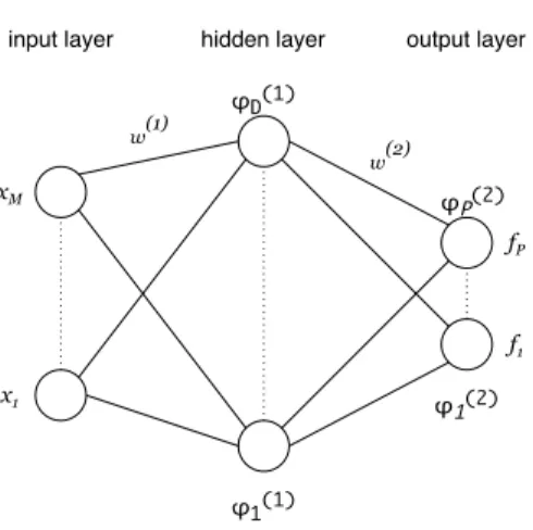
Feed Forward Neural Networks (FFNN), also known as multilayer percep-trons (MLP), are the most common type of neural networks in practical appli-cations. To explain this model we begin with a simple two layer FFNN model. Assume that we haveDbasis functions and our objective is to learn the param-eters of these basis functions together with the functionf discussed in Section 635
5.2.1. The form of the classification or regression task is
f(x, w(1), w(2)) =φ(2)(φ(1)(xTw(1))Tw(2)) (11) wherew(1) = (w(1) 1 , . . . , w (1) M ) T,φ(1)= (φ(1) 1 , . . . , φ (1) D ) T,w(2)= (w(2) 1 , . . . , w (2) D ) T, andφ(2)= (φ(2) 1 , . . . , φ (2) P )
T. Figure 3 visualizes this FFNN model. The elements
of input vector xare units (neurons) in the input layer, φ(1)i are the units in the hidden layer, and φ(2)i are the units in the output layer which outputs f. 640
Note that the activities of the units in each layer are a nonlinear function of the activities in the previous layer. In machine learning literature,φ(.) is also called activation function. The activation function in the last layer is chosen with respect to the data processing task. For example, for regression task we use linear activation and for multiclass classification we usesoftmax activation 645
function [57, 91, 55].
With enough hidden units, an FFNN with at least two layers can approx-imate an arbitrary mapping from a finite input space to a finite output space [121, 122, 123]. However, for an FFNN, finding the optimum set of weightswis 650
an NP-complete problem [124]. To train the model, there is a variety range of learning methods such as stochastic gradient descent, adaptive delta, adaptive gradient, adaptive moment estimation, Nesterov’s accelerated gradient and RM-Sprob. To improve the generalization of the model and reduce overfitting, there are a range of methods such as weight decay, weight-sharing, early stopping, 655
Figure 3: A two layers feed forward neural network. Note that each output neuron is connected to each input neuron, i.e., it is a fully connected neural network.
A two layer FFNN has the properties of restricted representation and gener-alization. Moreover, compactly represented functions withllayers may require exponential size with l−1 layers. Therefore, an alternative approach would 660
be an FFNN with more than one hidden layers, i.e., adeep neural network, in which different high-level features share low-level features [93, 90]. Significant results with deep neural networks have led them to be the most commonly used classifiers in machine learning [125, 57]. [126] present the method to forecast the states of IoT elements based on an artificial neural network. The presented 665
architecture of the neural network is a combination of a multilayered percep-tron and a probabilistic neural network. Also, [21] use FFNN for processing the health data.
5.7. Time Series and Sequential Data
So far in this article, the discussed algorithms dealt with set of data points 670
that are independent and identically distributed (i.i.d.). However, the set of data points are not i.i.d. for many cases, often resulting from time series mea-surements, such as the daily closing value of the Dow Jones Industrial Average and acoustic features at successive time frames. An example of non i.i.d set of data points in a context other than a time series is a character sequence in 675
a German sentence. In these cases, data points consist of sequences of (x, y) pairs rather than being drawn i.i.d. from a joint distributionp(x,y) and the sequences exhibit significant sequential correlation [127, 55].
In a sequential supervised learning problem, when data points are sequen-680
tial, we are given a training set{(xi, yi)}Ni=1 consisting of N samples and each
of them is a pair of sequences. In each sample, xi = hxi,1, xi,2, . . . , xi,Tii and
yi = hyi,1, yi,2, . . . , yi,Tii. Given a new, unseen input sequence x, the goal is
to predict the desired output sequencey. Moreover, there is a closely related problem, called atime-series prediction problem, in which the goal is to pre-685
dict the desired t+ 1st element of a sequencehy1, . . . , yti. The key difference
between them is that unlike sequential supervised learning, where the entire se-quencehx1, . . . , xTiis available prior to any prediction, in time-series prediction
only the prefix of the sequence, up to the current timet+ 1, is available. In addition, in sequential supervised learning, the entire output sequenceyhas to 690
be predicted, whereas in time-series prediction, the true observed values of the output sequence up to timetare given. It is worth noting that there is another closely-related task, calledsequence classification, in which the goal is to predict the desired, single categorical outputygiven an input sequencex[127]. 695
There are a variety of machine learning models and methods which can deal with these tasks. Examples of these models and methods are hidden Markov models [128, 129], sliding-window methods [130], Kalman filter [131], conditional random fields [132], recurrent neural networks [133, 57], graph transformer net-works [89], and maximum entropy Markov models [134]. In addition, sequential 700
time series and sequential data exists in many real world applications, including speech recognition [135], handwriting recognition [136], musical score following [137], and information extraction [134].
5.8. Anomaly Detection
The problem of identifying items or patterns in the data set that do not 705
conform to other items or an expected pattern is referred to as anomaly de-tection and these unexpected patterns are called anomalies, outliers, novelties, exceptions, noise, surprises, or deviations [138, 139].
There are many challenges in the task of anomaly detection which distin-710
guish it from a binary classification task. For example, an anomalous class is often severely underrepresented in the training set. In addition, anomalies are much more diverse than the behavior of the normal system and are sparse by nature [140, 139].
715
There are three broad categories of anomaly detection techniques based on the extent to which the labels are available. In supervised anomaly detection techniques, a binary (abnormal and normal) labeled data set is given, then, a binary classifier is trained; this should deal with the problem of theunbalanced data setdue to the existence of few data points with the abnormal label. Semi-720
supervised anomaly detection techniques require a training set that contains only normal data points. Anomalies are then detected by building the normal behavior model of the system and then testing the likelihood of the generation of the test data point by the learned model. Unsupervised anomaly detection techniques deal with an unlabeled data set by making the implicit assumption 725
that the majority of the data points are normal [139].
Anomaly detection is of use in many real world applications such as system health monitoring, credit card fraud detection, intrusion detection [141], de-tecting eco-system disturbances, and military surveillance. Moreover, anomaly 730
detection can be used as a preprocessing algorithm for removing outliers from the data set, that can significantly improve the performance of the subsequent machine learning algorithms, especially in supervised learning tasks [142, 143]. In the following subsection we shall explainone-class support vector machines
one of the most popular techniques for anomaly detection. [45] build a novel 735
outlier detection algorithm that uses statistical techniques to identify outliers and anomalies in power datasets collected from smart environments.
5.8.1. One-class Support Vector Machines
One-class support vector machines (OCSVMs) are a semi-supervised anomaly detection technique and are an extension of the SVMs discussed in Section 5.1.3 740
for unlabeled data sets. Given a training set drawn from an underlying probabil-ity distributionP, OCSVMs aim to estimate a subsetSof the input space such that the probability that a drawn sample fromP lies outside ofSis bounded by a fixed value between 0 and 1. This problem is approached by learning a binary functionf which captures the input regions where the probability density lives. 745
Therefore,f is negative in the complement ofS. The functional form off can be computed by solving a quadratic programming problem [94, 95].
One-class SVMs are useful in many anomaly detection applications, such as anomaly detection in sensor networks [144], system called intrusion detec-750
tion [145], network intrusions detection [146], and anomaly detection in wireless sensor networks [147]. [52] reviewed different techniques of stream data outlier detection and their issues in detail. [53] use One-class SVM to detect anomalies by modeling the complex normal patterns in the data.
In the following section, we discussed how to overcome the challenges of 755
applying machine learning algorithms to the IoT smart data.
6. Discussion on taxonomy of machine learning algorithms
In order to draw the right decisions for smart data analysis, it is necessary to determine which one of the tasks whether structure discovery, finding unusual data points, predicting values, predicting categories, or feature extraction should 760
be accomplished.
To discover the structure of data, the one that faces with the unlabeled data, the clustering algorithms can be the most appropriate tools. K-means described
in 5.4.1 is the well-known and frequently applied clustering algorithm, which can handle a large volume of data with a broad range of data types. [50, 52] 765
proposed a method for applying K-means algorithm in managing the Smart City and Smart Home data. DB-scan described in 5.4.2 is another clustering algorithm to discover the structure of data from the unlabeled data which is applied in [109, 52, 47] to cluster Smart Citizen behaviors.
To find unusual data points and anomalies in smart data, two important 770
algorithms are applied. One class Support Vector Machine and PCA based anomaly detection methods explained in 5.5.1 which have the ability to train anomaly and noisy data with a high performance. [52, 53] applied the One class SVM monitor and find the human activity anomalies.
In order to predict values and classification of sequenced data, Linear re-775
gression and SVR described in 5.2.1 and 5.2.2 are the two frequently applied algorithms. The objective of the models applied in these algorithms is to process and train data of high velocity. For example [48, 46] applied linear regression algorithm for real-time prediction. Another fast training algorithm is the clas-sification and regression tree described in 5.3.1, applied in classifying Smart 780
Citizen behaviors [48, 47].
To predict the categories of the data, neural networks are proper learning models for function approximation problems. Moreover, because the smart data should be accurate and it takes a long time to be trained, the multi-class neural network can be an appropriate solution. For instance, Feed Froward Neural 785
Network explained in 5.6.1 applied to reduce energy consumption in future by predicting how the data in future will be generated and how the redundancy of the data would be removed [21, 126, 148]. SVM explained in 5.1.3 is another popular classification algorithm capable of handling massive amounts of data and classify their different types. Because SVM solves the high volume and the 790
variety types of data, it is commonly applied in most smart data processing algorithms. For example, [109, 48] applied SVM to classify the traffic data.
PCA and CCA described in 5.5.1 and 5.5.2 are the two algorithms vastly applied in extracting features of the data. Moreover, CCA shows the correlation
between the two categories of the data. A type of PCA and CCA are applied to 795
finding the anomalies. [51] applied PCA and CCA to monitor the public places and detect the events in the social areas.
The chosen algorithm should be implemented and developed to make right decisions.
A sample implemented code is available from the open source GitHub license 800
at https://github.com/mhrezvan/SVM-on-Smart-Traffic-Data
7. Research trends and open issues
As discussed before, data analysis have a significant contribution to IoT; therefore to applied a full potential of analysis to extract new insights from data, IoT must overcome some major problems. These problems can be categorized 805
in three different types.
7.1. IoT Data Characteristics
Because the data are the basis of extracting knowledge, it is vital to have high quality information. This condition can affect the accuracy of knowledge extraction in a direct manner. Since IoT produces high volume, fast velocity, 810
and varieties of data, preserving the data quality is a hard and challenging task. Although many solutions have been and are being introduced to solve these problems, none of them can handle all aspects of data characteristics in an accurate manner because of the distributed nature of Big Data management solutions and real-time processing platforms. The abstraction of IoT data is 815
low, that is, the data that comes from different resources in IoT are mostly of raw data and not sufficient enough for analysis. A wide variety of solutions are proposed, while most of them need further improvements. For instance, seman-tic technologies tend to enhance the abstraction of IoT data through annotation algorithms, while they need more efforts to overcome its velocity and volume. 820
7.2. IoT Applications
IoT applications have different categories according to their unique attribu-tions and features. Certain issues should be proposed in running data analysis in IoT applications in an accurate manner. First, the privacy of the collected data is very critical, since data collection process can include personal or critical 825
business data, which is inevitable to solve the privacy issues. Second, according to the vast number of resources and simple-designed hardware in IoT, it is vi-tal to consider security parameters like network security, data encryption, etc. Otherwise, by ignoring the security in design and implementation, an infected network of IoT devices can cause a crisis.
830
7.3. IoT Data Analytics Algorithms
According to the smart data characteristics, analytic algorithms should be able to handle Big Data, that is, IoT needs algorithms that can analyze the data which comes from a variety of sources in real time. Many attempts are made to address this issue. For example, deep learning algorithms, evolutionized form 835
of neural networks can reach to a high accuracy rate if they have enough data and time. Deep learning algorithms can be easily influenced by the smart noisy data, furthermore, neural network based algorithms lack interpretation, this is, data scientists can not understand the reasons for the model results. In the same manner, semi-supervised algorithms which model the small amount of labeled 840
data with a large amount of unlabeled data can assist IoT data analytics as well.
8. Conclusions
IoT consists of a vast number of devices with varieties that are connected to each other and transmit huge amounts of data. The Smart City is one of the 845
most important applications of IoT and provides different services in domains like energy, mobility, and urban planning. These services can be enhanced and optimized by analyzing the smart data collected from these areas. In order to
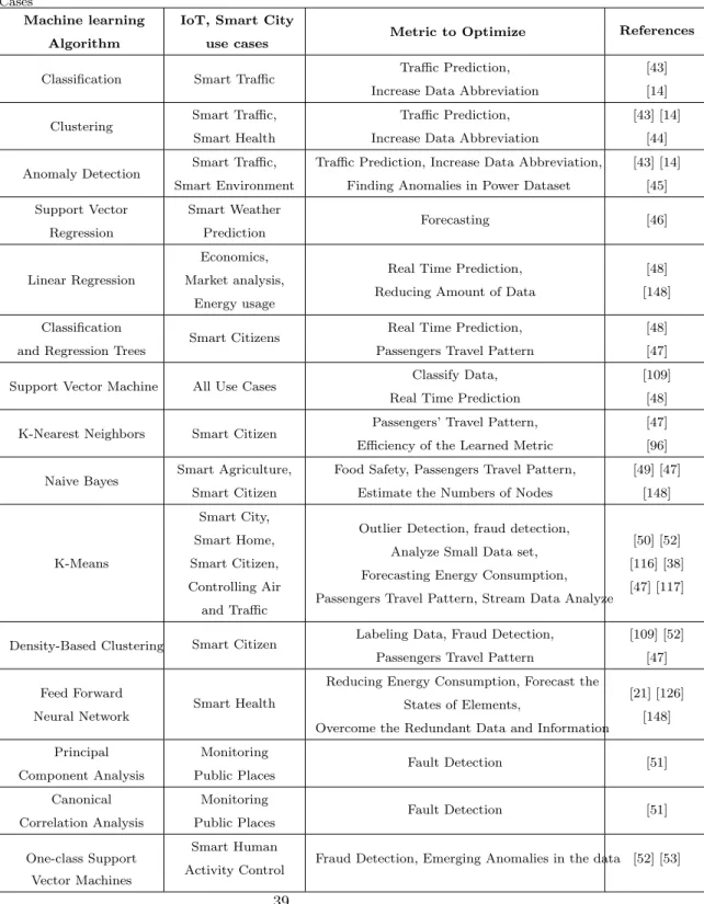
Table 3: Overview of Applying Machine Learning Algorithm to the Internet of Things Use Cases
Machine learning Algorithm
IoT, Smart City
use cases Metric to Optimize
References
Classification Smart Traffic Traffic Prediction, Increase Data Abbreviation
[43] [14]
Clustering Smart Traffic, Smart Health
Traffic Prediction, Increase Data Abbreviation
[43] [14] [44]
Anomaly Detection Smart Traffic, Smart Environment
Traffic Prediction, Increase Data Abbreviation, Finding Anomalies in Power Dataset
[43] [14] [45] Support Vector Regression Smart Weather Prediction Forecasting [46] Linear Regression Economics, Market analysis, Energy usage
Real Time Prediction, Reducing Amount of Data
[48] [148]
Classification and Regression Trees
Smart Citizens Real Time Prediction, Passengers Travel Pattern
[48] [47]
Support Vector Machine All Use Cases Classify Data, Real Time Prediction
[109] [48]
K-Nearest Neighbors Smart Citizen Passengers’ Travel Pattern, Efficiency of the Learned Metric
[47] [96]
Naive Bayes Smart Agriculture, Smart Citizen
Food Safety, Passengers Travel Pattern, Estimate the Numbers of Nodes
[49] [47] [148] K-Means Smart City, Smart Home, Smart Citizen, Controlling Air and Traffic
Outlier Detection, fraud detection, Analyze Small Data set, Forecasting Energy Consumption, Passengers Travel Pattern, Stream Data Analyze
[50] [52] [116] [38] [47] [117]
Density-Based Clustering Smart Citizen Labeling Data, Fraud Detection, Passengers Travel Pattern
[109] [52] [47]
Feed Forward Neural Network
Smart Health
Reducing Energy Consumption, Forecast the States of Elements,
Overcome the Redundant Data and Information
[21] [126] [148] Principal Component Analysis Monitoring Public Places Fault Detection [51] Canonical Correlation Analysis Monitoring Public Places Fault Detection [51] One-class Support Vector Machines Smart Human