End-to-End Machine Learning Frameworks for Medicine: Data Imputation, Model Interpretation and Synthetic Data Generation

(1)

UCLA

UCLA Electronic Theses and Dissertations

Permalink https://escholarship.org/uc/item/2q51g25p Author Yoon, Jinsung Publication Date 2020 Peer reviewed|Thesis/dissertation

(2)

UNIVERSITY OF CALIFORNIA Los Angeles

End-to-End Machine Learning Frameworks for Medicine:

Data Imputation, Model Interpretation and Synthetic Data Generation

A dissertation submitted in partial satisfaction of the requirements for the degree

Doctor of Philosophy in Electrical and Computer Engineering

by

Jinsung Yoon

(3)

c

Copyright by Jinsung Yoon

(4)

ABSTRACT OF THE DISSERTATION

End-to-End Machine Learning Frameworks for Medicine:

Data Imputation, Model Interpretation and Synthetic Data Generation

by

Jinsung Yoon

Doctor of Philosophy in Electrical and Computer Engineering University of California, Los Angeles, 2020

Professor Mihaela van der Schaar, Chair

Tremendous successes in machine learning have been achieved in a variety of applications such as image classification and language translation via supervised learning frameworks. Recently, with the rapid increase of electronic health records (EHR), machine learning researchers got immense opportunities to adopt the successful supervised learning frameworks to diverse clinical applications. To properly employ machine learning frameworks for medicine, we need to handle the special properties of the EHR and clinical applications: (1) extensive missing data, (2) model interpretation, (3) privacy of the data. This dissertation addresses those specialties to construct end-to-end machine learning frameworks for clinical decision support.

We focus on the following three problems: (1) how to deal with incomplete data (data imputation), (2) how to explain the decisions of the trained model (model interpretation), (3) how to generate synthetic data for better sharing private clinical data (synthetic data generation). To appropriately handle those problems, we propose novel machine learning algorithms for both static and longitudinal settings. For data imputation, we propose modified Generative Adversarial Networks and Recurrent Neural Networks to accurately impute the missing values and return the complete data for applying state-of-the-art supervised learning models. For model interpretation, we utilize the actor-critic framework to estimate feature importance of the trained model’s decision in an instance level. We expand this algorithm to active sensing framework that recommends which observations should we measure and

(5)

when. For synthetic data generation, we extend well-known Generative Adversarial Network frameworks from static setting to longitudinal setting, and propose a novel differentially private synthetic data generation framework.

To demonstrate the utilities of the proposed models, we evaluate those models on various real-world medical datasets including cohorts in the intensive care units, wards, and primary care hospitals. We show that the proposed algorithms consistently outperform state-of-the-art for handling missing data, understanding the trained model, and generating private synthetic data that are critical for building end-to-end machine learning frameworks for medicine.

(6)

The dissertation of Jinsung Yoon is approved.

Gregory J. Pottie

Jonathan Chau-Yan Kao

William Hsu

Mihaela van der Schaar, Committee Chair

University of California, Los Angeles

(7)

(8)

LIST OF FIGURES

1.1 End-to-end machine learning pipeline in longitudinal setting. (1) Data preprocess-ing (includpreprocess-ing imputation), (2) Model trainpreprocess-ing, (3) Model interpretation. . . 3

1.2 Synthetic data generation for sharing the private medical data to machine learning community for developing machine learning tools easier. . . 5

2.1 The architecture of GAIN with exemplar samples. . . 13

2.2 RMSE performance in different settings: (a) Various missing rates, (b) Various number of samples, (c) Various feature dimensions . . . 24

2.3 The AUROC performance with various missing rates with Credit dataset . . . . 28

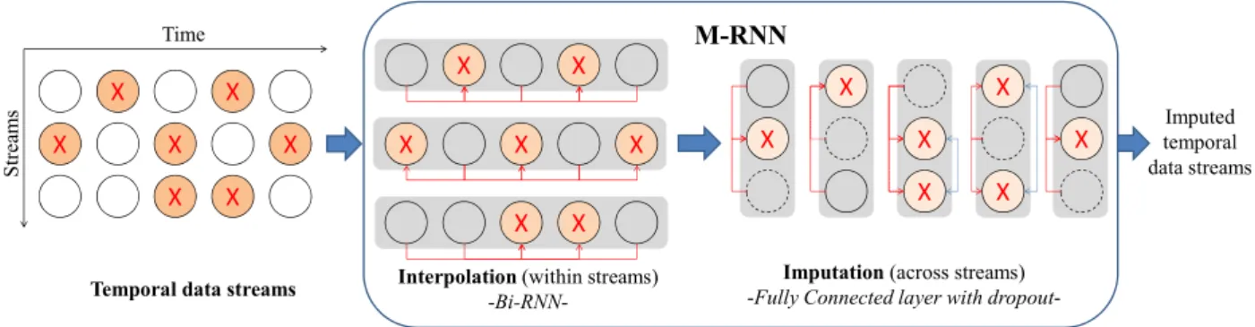
3.1 Block diagram of missing data estimation process. X: missing measurements; red lines: connections between observed values and missing values in each layer; blue lines: connections between interpolated values; dashed lines: dropout . . . 31

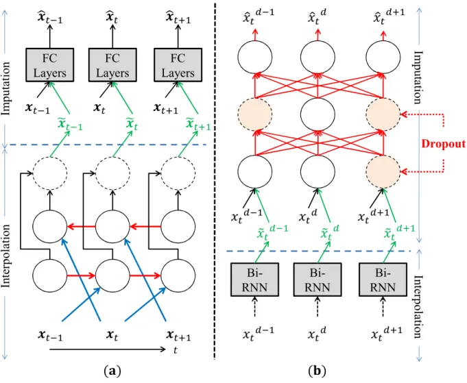
3.2 M-RNN Architecture. (a) Architecture in the time domain section; (b) Architec-ture in the feaArchitec-ture domain section (Dropout is used for multiple imputations). Note that both ˜x (the output of interpolation block) and x are inputs to the imputation block to construct ˆx (the output of imputation block). . . 40 3.3 Box-plot comparisons between M-RNN (MI), M-RNN (SI) and the best benchmark.

(a) RMSE comparison using MIMIC-III dataset, (b) AUROC comparison using MIMIC-III dataset. Red crosses represents outliers. . . 45

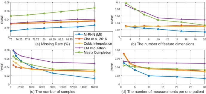
3.4 Imputation accuracy for the MIMIC-III dataset with various settings (a) Additional data missing at random, (b) Feature dimensions chosen at random, (c) Samples chosen at random, (d) Measurements chosen at random . . . 47

3.5 (a) The AUROC performance with various missing rates, (b) The AUROC gain over the two most competitive benchmarks . . . 51

(14)

4.1 Block diagram of INVASE. Instances are fed into the selector network which outputs a vector of selection probabilities. The selection vector is then sampled according to these probabilities. The predictor network then receives the selected features and makes a prediction and the baseline network is given the entire feature vector and makes a prediction. Each of these networks are trained using backpropagation using the real label. The loss of the baseline network is then subtracted from the prediction network’s loss and this is used to update the selector network. . . 63

4.2 Left: The feature importance for each of 20 randomly selected patients in the MAGGIC dataset. Right: The average feature importance for different binary splits in the MAGGIC dataset. . . 72

5.1 Comparison of active sensing and instance-wise variable selection in the static setting. . . 76

5.2 Comparison of active sensing and instance-wise variable selection in the time-series setting. . . 77

5.3 Block diagram of ASAC. . . 84

5.4 Block diagram of ASAC in a time-series setting. . . 88

5.5 Results on risk predictions on both ADNI and MIMIC-III dataset with various cost constraints in terms of AUROC and AUPRC. X-axis is cost constraints (rate of selected measurements). Y-axis is predictive performance. . . 91

6.1 (a) Block diagram of component functions and objectives. (b) Training scheme; solid lines indicate forward propagation of data, and dashed lines indicate back-propagation of gradients. . . 102

6.2 (a) TimeGAN instantiated with RNNs, (b) C-RNN-GAN, and (c) RCGAN. Solid lines denote function application, dashed lines denote recurrence, and orange lines indicate loss computation. . . 105

(15)

6.3 t-SNE visualization on Sines (1st _{row) and Stocks (2}nd _{row). Each column provides}

the visualization for each of the 7 benchmarks. Red denotes original data, and blue denotes synthetic. . . 112

7.1 Block diagram of the training procedure for the teacher-discriminator during a single generator iteration. Teacher-discriminators are trained to minimize the classification loss when classifying samples as real samples or generated samples. During this step only the parameters of the teachers are updates (and not the generator). . . 124

7.2 Block diagram of the training procedure for the student-discriminator and the generator. The student-discriminator is trained using noisy teacher-labelled generated samples (the noise provides the DP guarantees). The student is trained to minimize classification loss on this noisily labelled dataset, while the generator is trained to maximize the student loss. Note that the teachers are not updated during this step, only the student and the generator. . . 125

7.3 Average AUROC performance across 12 different predictive models trained on the synthetic dataset generated by PATE-GAN and DPGAN with various (with δ = 10−5) (Setting B). . . 131

(16)

LIST OF TABLES

2.1 Source of gains in GAIN algorithm (Mean _± Std of RMSE (Gain (%))) . . . 22 2.2 Statistics of the datasets. Scont: the number of continuous variables, Scat: the

number of categorical variables . . . 23

2.3 Imputation performance in terms of RMSE (Average _±Std of RMSE) . . . 24 2.4 Imputation performance with uniform and non-uniform pm(i) on MCAR, MAR,

and MNAR (Average _± Std of RMSE) settings. . . 26 2.5 Prediction performance comparison . . . 27

2.6 Congeniality performances of imputation models . . . 29

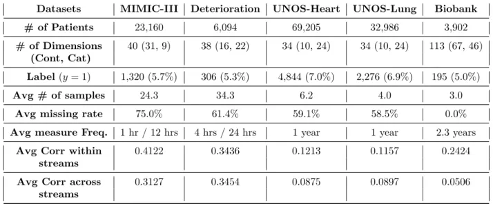
3.1 Summary of the datasets (Cont: Continuous, Cat: Categorical, Avg: Average, #: Number, Corr: Correlation, Freq: Frequency) . . . 42

3.2 Performance comparison for missing data estimation . . . 43

3.3 Performance comparison for joint interpolation/imputation algorithms . . . 45

3.4 Source of Gain of M-RNN. (Performance degradation from original M-RNN) . . 46

3.5 Performance comparison for patient state prediction with a 1-layer RNN (Perfor-mance gain is computed in terms of 1-AUROC) . . . 50

3.6 Congeniality of imputation models . . . 54

3.7 Performance comparison for missing data estimation for MCAR and MAR settings on the Biobank dataset . . . 55

4.1 Relevant feature discovery results for Synthetic datasets with 11 features . . . . 67

4.2 Detailed comparison of INVASE with L2X in Syn4 and Syn5, highlighting the capability of INVASE to select a flexible number of features for each sample. Group 1: X11 <0, Group 2: X11≥0 . . . 68

(17)

4.4 Prediction performance comparison with and without feature selection methods (L2X, LASSO, Tree, INVASE, and Global). Global is using ground-truth globally

relevant features for each dataset . . . 70

4.5 Selection probability of overall and patient subgroups by INVASE in MAGGIC dataset. (Mean _± Std) . . . 72 4.6 Prediction performance for MAGGIC and PLCO dataset. . . 73

4.7 Predictive Performance Comparison on two real-world datasets (MAGGIC and PLCO) in terms of AUROC and AUPRC . . . 74

5.1 Comparison of related works. Causal refers to whether or not a selection depends on future selections or not. . . 80

5.2 Measurement rate of each feature when each feature has a different auto-regressive coefficient. . . 93

5.3 Measurement rate based on different cost and noise parameter γ for original feature (Xt) and noisy feature ( ˆXt). . . 94

5.4 Measurement rate when the cost is different for Yt= 1 and Yt= 0. . . 95

6.1 Summary of Related Work. (Open-loop: Previous outputs are used as conditioning information for generation at each step; Mixed-variables: Accommodates static & temporal variables). . . 101

6.2 Results on autoregressive multivariate Gaussian data (Bold indicates best perfor-mance). . . 111

6.3 Dataset statistics . . . 111

6.4 Results on multiple time-series datasets (Bold indicates best performance). . . . 113

6.5 Source-of-gain analysis on multiple datasets (via discriminative and predictive scores). . . 114

(18)

7.1 No of samples, No of features, Average AUROC and AUPRC performance across 12 different predictive models trained and tested on the real data (Setting A) for the 6 datasets: Kaggle Credit, MAGGIC, UNOS, Kaggle Cervical Cancer, UCI ISOLET, UCI Epileptic Seizure Recognition. . . 128

7.2 Performance comparison of 12 different predictive models in Setting B (trained on synthetic, tested on real) in terms of AUROC and AUPRC (the generators of PATE-GAN and DPGAN are (1,10−5_{)-differentially private). . . 129}

7.3 Performance comparison of 12 different predictive models in Setting B (trained on synthetic, tested on real) in terms of AUROC and AUPRC (the generators of PATE-GAN and DPGAN are (1,10−5)-differentially private) over 6 different datasets. GAN is (_∞,_∞)-differentially private and is given to indicate an upper bound of PATE-GAN and DPGAN. . . 130

7.4 Synthetic Ranking Probability of PATE-GAN and the benchmark when comparing Setting A and Setting C for various (with δ= 10−5_{) in terms of AUROC. The}

Synthetic Ranking Agreement of Original GAN is 0.9091, which is also attained by both PATE-GAN and DPGAN for = 50. . . 132

7.5 Agreed ranking probability of PATE-GAN and the benchmark to order the features by variable importance in terms of absolute Pearson correlation coefficient . . . 133

(19)

ACKNOWLEDGMENTS

It would not have been possible to complete this doctoral dissertation without the help and support of the kind people around me. I am deeply grateful.

First, I would like to express the deepest appreciation to my advisor, Professor Mihaela van der Schaar, for her expertise, assistance, and patience throughout my entire PhD research. Her unwavering enthusiasm for research kept me constantly engaged with my research on developing diverse machine learning algorithms for medicine. Without her devoted guidance, persistent help, and insightful research directions, this dissertation would not have been possible. I would also thank my dissertation committee members, Professor Gregory Pottie, Professor Jonathan Kao, and Professor William Hsu for their thoughtful suggestions and considerate comments.

My sincere thanks also goes to all of my colleagues. I have been lucky to spend some time in Europe as a recognized student at University of Oxford; thus, my colleagues are spread around the globe. I would like to thank all of my co-authors; Professor William Zame, Professor Cem Tekin, Dr. Ahmed Alaa, Changhee Lee, and Kyeong Ho Kenneth Moon at UCLA; James Jordon at University of Oxford; Daniel Jarrett, Yao Zhang, and Dr. Lydia Drumright at University of Cambridge. It has been a great honor to collaborate with such brilliant people. I would also like to thank all of my lab mates; Dr. William Whoiles, Dr. Kartik Ahuja, and Trent Kyono at UCLA; Ioana Bica at University of Oxford; Alexis Bellot, Alihan Huyuk, and Zhaozhi Qian at University of Cambridge for their critical comments and passionate research discussions.

I was fortunate to collaborate with many clinicians who tremendously help transforming my research into real-world clinical applications. I would like to thank Professor Raffaele Bugiardini (University of Bologna, Italy) for providing precious clinical datasets across the entire Europe, guiding to come up with the vital clinical discovery, and publishing high-impact clinical journals such as JAMA Internal Medicine. I would also like to thank other clinical collaborators; Dr. Scott Hu, Dr. Camelia Davtyan, Dr. Martin Cadeiras, and Dr. Mindy Ross at UCLA; Dr. Lydia Drumright and Dr. Ari Ercole at University of Cambridge for

(20)

their sympathetic clinical comments and suggestions on my research.

Finally, and most importantly, I wish to thank my parents, my brother’s family, and my love, for their endless support. I have no valuable words to express my thanks for their spiritual supports throughout my entire graduate education.

(21)

VITA

2014 Bachelor in Electrical Engineering and Computer Engineering Department, Seoul National University, Seoul, Korea

2016 Master of Science in Electrical and Computer Engineering Department, University of California, Los Angeles, United States

2015–2020 Graduate Student Researcher in Electrical and Computer Engineering Department, University of California, Los Angeles, United States.

2015–2016 Teaching Assistant, Electrical and Computer Engineering Department, University of California, Los Angeles, United States.

2016 Outstanding Master Thesis, Electrical and Computer Engineering Depart-ment, University of California, Los Angeles, United States.

2017–2018 Recognized Student, Engineering Science Department, University of Oxford, Oxfordshire, United Kingdom.

2019 Research Intern, Google Cloud AI, California, United States.

PUBLICATIONS

J. Yoon, L. N. Drumright, M. van der Schaar, “ Anonymization through Data Synthesis using Generative Adversarial Networks (ADS-GAN),” IEEE J. Biomedical and Health Informatics

(JBHI), 2020.

J. Yoon, D. Jarrett, M. van der Schaar, “Time-series Generative Adversarial Networks,”

Neural Information Processing Systems (NeurIPS), 2019.

J. Yoon, J. Jordon, M. van der Schaar, “INVASE: Instance-wise Variable Selection using Neural Networks,” International Conference on Learning Representations (ICLR), 2019.

(22)

J. Yoon, J. Jordon, M. van der Schaar, “PATE-GAN: Generating Synthetic Data with Differential Privacy Guarantees,” International Conference on Learning Representations

(ICLR), 2019.

J. Yoon, J. Jordon, M. van der Schaar, “GAIN: Missing Data Imputation using Generative Adversarial Nets,” International Conference on Machine Learning (ICML), 2018.

J. Yoon, J. Jordon, M. van der Schaar, “RadialGAN: Leveraging Multiple Datasets to Improve Target-specific Predictive Models using Generative Adversarial Networks,” Interna-tional Conference on Machine Learning (ICML), 2018.

J. Yoon, J. Jordon, M. van der Schaar, “GANITE: Estimation of Individualized Treatment Effects using Generative Adversarial nets,” International Conference on Learning Represen-tations (ICLR), 2018.

J. Yoon, W. R. Zame, M. van der Schaar, “Deep Sensing: Active Sensing using Multi-directional Recurrent Neural Networks,”International Conference on Learning Representa-tions (ICLR), 2018.

J. Yoon, W. R. Zame, A. Banerjee, M. Cadeiras, A. M. Alaa, M. van der Schaar, “Personal-ized Survival Predictions via Trees of Predictors: An Application to Cardiac Transplantation,”

PloS One, 2018.

J. Yoon, W. R. Zame, M. van der Schaar, “Estimating Missing Data in Temporal Data Streams using Multi-directional Recurrent Neural Networks,” IEEE Transactions on Biomed-ical Engineering (TBME), 2018.

J. Yoon, W. R. Zame, M. van der Schaar, “ToPs: Ensemble Learning with Trees of Predic-tors,” IEEE Transactions on Signal Processing (TSP), 2018.

J. Yoon, A. M. Alaa, M. Cadeiras, M. van der Schaar, “Personalized Donor-Recipient Matching for Organ Transplantation,” AAAI, 2017.

J. Yoon, A. M. Alaa, S. Hu, M. van der Schaar, “ForecastICU: A Prognostic Decision Support System for Timely Prediction of Intensive Care Unit Admission,” International Conference on Machine Learning (ICML), 2016.

J. Yoon, C. Davtyan, M. van der Schaar, “Discovery and Clinical Decision Support for Personalized Healthcare,” IEEE Journal of Biomedical and Health Informatics (JBHI), 2015.

(23)

CHAPTER 1

Introduction

With the advent of electronic health records (EHR), the collections of clinical data are rapidly increased for numerous patients across the entire world. Simultaneously, data-driven machine learning frameworks have been achieved enormous successes in a variety of applications (such as image classification [HZR16], object detection [HGD17], and language translation [VSP17]) with deep learning models via supervised learning frameworks.

The availability of various medical datasets and high performing machine learning frame-works results in extensive opportunities for developing diverse data-driven clinical decision support such as early warning systems [YAH16] and clinical risk scoring systems [AS18a]. However, unlike image and language domains, medical domain has its own characteristics that machine learning researchers must consider to constructing end-to-end machine learning frameworks for medicine.

First, missing data is ubiquitous in medical data. The missing data problem is especially challenging in medical domains which present time-series containing many streams of mea-surements that are sampled at different and irregular times [YZS18a]. This is significantly important because accurate estimation of these missing measurements is often critical for accurate diagnosis, prognosis [AS18b] and treatment, as well as for accurate modeling and statistical analyses [AYH18].

Second, clinical decision support should provide proper interpretations for its decisions. Medicine is more conservative field than computer vision and natural language. Without proper understanding of the trained models and explanations of their decisions, it is difficult to widely apply those models to real-world clinical decision support. Clinicians expect to get not only patient outcome predictions but also how those predictions are derived from clinical

(24)

decision support.

Third, medical data is usually private. Medical and machine learning communities are relying on the promise of artificial intelligence (AI) to transform medicine through enabling more accurate decisions and personalized treatment. However, progress is slow. Legal and ethical issues around unconsented patient data and privacy is one of the limiting factors in data sharing, resulting in a significant barrier in accessing routinely collected EHR by the machine learning community. To alleviate this difficulty, generating synthetic data that closely approximates the joint distribution of variables in an original EHR dataset can provide a readily accessible, legally and ethically appropriate solution to support more open data sharing, and enable the development of AI solutions.

In this Chapter, we illustrate the end-to-end machine learning pipeline for healthcare application, and synthetic data generation framework for private medical data sharing. Then, we summarize the contributions of the following chapters in this dissertation.

1.1

End-to-end machine learning pipeline for medicine

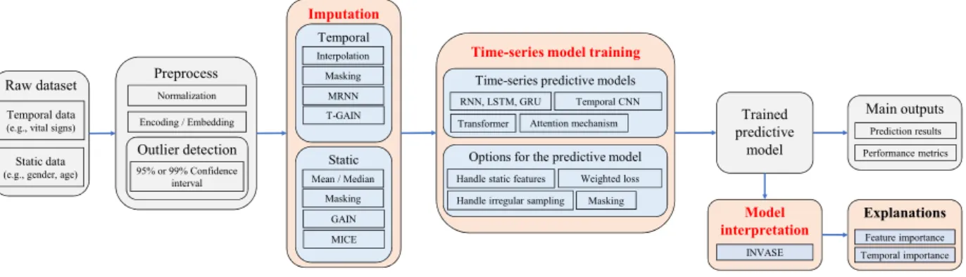
High-level end-to-end machine learning pipeline is made up of three stages: (1) Data prepro-cessing, (2) Model training, (3) Model interpretation. Most machine learning researchers focus on stage (2) - model training via supervised learning frameworks. For instance, popular image classification models such as ResNet [HZR16] and InceptionV3 [SVI16] are convolutional neural networks based supervised learning model for stage (2). On the other hand, stage (1) and stage (3) are under-explored even though those stages are critical in medicine. In this dissertation, we focus on developing novel and high-performing machine learning algorithms for stage (1) and (3). Fig. 1.1 illustrate the high-level abstractions of the end-to-end machine learning pipeline in longitudinal setting.

(25)

Raw dataset

Temporal data

(e.g., vital signs)

Static data

(e.g., gender, age)

Trained predictive model Main outputs Prediction results Model interpretation INVASE Explanations Feature importance Temporal importance Preprocess Normalization Encoding / Embedding Outlier detection 95% or 99% Confidence interval

Time-series model training

Time-series predictive models RNN, LSTM, GRU Temporal CNN Transformer

Options for the predictive model Handle static features Weighted loss

Attention mechanism

Handle irregular sampling Masking

Performance metrics Imputation Temporal Interpolation Masking MRNN Static Mean / Median Masking GAIN T-GAIN MICE

Figure 1.1: End-to-end machine learning pipeline in longitudinal setting. (1) Data prepro-cessing (including imputation), (2) Model training, (3) Model interpretation.

1.1.1 Data imputation

Missing data is a pervasive problem. Data may be missing for many reasons. For instance, in the medical domain, the respiratory rate of a patient may not have been measured (perhaps because it was deemed unnecessary/unimportant) or accidentally not recorded [YDS17, AYH18]. It may also be the case that certain pieces of information are difficult or even dangerous to acquire (such as information gathered from a biopsy), and so these were not gathered for those reasons [YZB18]. The critical part of the medical data preprocessing stage is how to deal with those missing values. Accurate estimation of the missing measurements is important for many reasons, including diagnosis, prognosis and treatment. Furthermore, most state-of-the-art machine learning models are only applicable when the input data is complete; thus, without proper handling of the missing data, we cannot move on to the next stage (training machine learning models) of the machine learning pipeline.

In Chapter 2 and 3, we propose state-of-the-art imputation models for static and lon-gitudinal settings. In Chapter 2, we propose a novel imputation method using modified Generative Adversarial Networks in static setting. In Chapter 3, we modified Recurrent Neural Networks for imputing missing data in longitudinal setting.

(26)

1.1.2 Model interpretation

State-of-the-art prediction performance is not the only expectation for clinical decision support. Reasonable explanations of the decisions are mandatory for doctors and patients to trust the clinical decision support. Moreover, understanding data-driven machine learning models for medicine can provide new insights on medicine which may result in the vital clinical discovery.

Defining the model interpretability is not straightforward, and there are various definitions of model interpretability such as symbolic modeling [AS19] and concept-based modeling [KWG17]. In this dissertation, we define the model interpretability as discovering instance-wise feature importance which is widely used interpretation definition [SGK17, CSW18].

In Chapter 4, we proposed an instance-wise feature selection method for interpreting the trained model using a novel actor-critic framework. This can provide an explanation (i.e. evidence or support) of the trained model’s individual decision.

In Chapter 5, we extend the instance-wise feature selection method to active sensing problem. In many medical settings, making observations is costly [WRG96]. For example, performing lab tests on a patient incurs a cost, both financially as well as causing fatigue to the patient [KBR09, KNS08]. In such settings, the decision to observe is important and should be an active choice. We propose a novel actor-critic model of recommending which measurements should we measure and when.

1.2

Synthetic data generation for private data sharing

The adoption of EHR has dramatically increased in high-income countries over the last decade [HPS17, KJP17, GH16] with corresponding interest to do so in low and middle income countries worldwide [LB15]. Evidence from both small scale studies and other disciplines suggests that machine learning could support significant advances in healthcare delivery [RFP19, TP18], however, appropriate legal and ethical management of routinely collected EHR can create obstacles to open sharing of sensitive health data.

(27)

Important Use Case

•

Enable to share the private (identifiable)

data (by sharing

de-identified synthetic data) to machine learning community to

develop machine learning tools easier.

3

Synthetic data

generation

Private

medical data

Synthetic

medical data

Deidentified

ML Community

Machine Learning Tools

Hospitals

Figure 1.2: Synthetic data generation for sharing the private medical data to machine learning community for developing machine learning tools easier.

Given the complicated dynamics around protecting, anonymizing and sharing routinely collected health data, we decided to address the problem in a new way. We developed a model to create entirely synthetic datasets of individuals that are fictious and yet could be drawn from the same population as the real dataset. Fig. 1.2 illustrates the simple block diagram of synthetic data generation for private data sharing between machine learning community and clinical data providers.

In Chapter 6, we extends well-known Generative Adversarial Networks for synthetic data generation from static setting to longitudinal setting. In Chapter 7, we proposed a differentially private synthetic data generation framework where differential privacy is well-defined mathematical notion of the privacy [DR14].

1.3

Summary of contributions

(28)

1.3.1 Chapter 2 contributions

In Chapter 2, we consider the missing data imputation problem in static setting. We propose a novel method for imputing missing data by adapting the well-known Generative Adversarial Nets (GAN) framework. The generator observes some components of a real data vector, imputes the missing components conditioned on what is actually observed, and outputs a completed vector. The discriminator then takes a completed vector and attempts to determine which components were actually observed and which were imputed. To ensure that the discriminator forces the generator to learn the desired distribution, we provide the discriminator with some additional information in the form of a hint vector. The hint reveals to the discriminator partial information about the missingness of the original sample, which is used by the discriminator to focus its attention on the imputation quality of particular components. This hint ensures that the generator does in fact learn to generate according to the true data distribution.

In Chapter 3, we address the missing data imputation problem in longitudinal setting. Existing methods address this estimation problem by interpolating within data streams or imputing across data streams (both of which ignore important information) or ignoring the temporal aspect of the data and imposing strong assumptions about the nature of the data-generating process and/or the pattern of missing data (both of which are especially problematic for medical data). We propose a new approach, based on a novel deep learning architecture that interpolates within data streams and imputes across data streams.

In Chapter 4, we tackle the model interpretation problem in static setting where we define the interpretation as estimating instance-wise feature importance for individual prediction. We propose a new instance-wise feature selection method. The proposed model consists of 3 neural networks, a selector network, a predictor network and a baseline network which are

(29)

used to train the selector network using the actor-critic framework. Using this methodology, the proposed model is capable of flexibly discovering feature subsets of a different size for each instance, which is a key limitation of existing state-of-the-art methods.

In Chapter 5, we extend the instance-wise feature selection methodology to active sensing problem in the longitudinal setting. Deciding what and when to observe is critical when making observations is costly. In a medical setting where observations can be made sequentially, making these observations (or not) should be an active choice. We propose a novel deep learning framework to address this problem. The proposed model consists of two networks: a selector network and a predictor network. The selector network uses previously selected observations to determine what should be observed in the future. The predictor network uses the observations selected by the selector network to predict a label, providing feedback to the selector network (well-selected variables should be predictive of the label). The goal of the selector network is then to select variables that balance the cost of observing the selected variables with their predictive power.

In Chapter 6, we study the synthetic data generation problem in longitudinal setting. A good generative model for time-series data should preserve temporal dynamics, in the sense that new sequences respect the original relationships between variables across time. Existing methods that bring GANs into the sequential setting do not adequately attend to the temporal correlations unique to time-series data. At the same time, supervised models for sequence prediction - which allow finer control over network dynamics - are inherently deterministic. We propose a novel framework for generating realistic time-series data that combines the flexibility of the unsupervised paradigm with the control afforded by supervised training. Through a learned embedding space jointly optimized with both supervised and adversarial objectives, we encourage the network to adhere to the dynamics of the training data during

(30)

sampling.

In Chapter 7, we focus on the private synthetic data generation problem in static setting. We investigate a method for ensuring differential privacy of the generator of the GAN framework. The resulting model can be used for generating synthetic data on which algorithms can be trained and validated, and on which competitions can be conducted, without compromising the privacy of the original dataset. Our method modifies the Private Aggregation of Teacher Ensembles framework and applies it to GANs. We also look at measuring the quality of synthetic data from a new angle; we assert that for the synthetic data to be useful for machine learning researchers, the relative performance of two algorithms (trained and tested) on the synthetic dataset should be the same as their relative performance (when trained and tested) on the original dataset.

(31)

CHAPTER 2

GAIN: Missing Data Imputation using Generative

Adversarial Nets

Missing values are prevalent in medical data. Data may be missing because it was never collected, records were lost or for many other reasons. An imputation algorithm can be used to estimate missing values based on data that was observed/measured, such as the systolic blood pressure and heart rate of the patient [YZS18a]. A substantial amount of research has been dedicated to developing imputation algorithms for medical data [BM99, Mac10, SWC09, PS15]. Imputation algorithms are also used in many other applications such as image concealment, data compression, and counterfactual estimation [Rub04, KL12, YJS18].

State-of-the-art imputation methods can be categorized as either discriminative or gen-erative. Discriminative methods include MICE [WRW11, BG11], MissForest [SB11], and matrix completion [CR09, YRD16, SSS16]; generative methods include algorithms based on Expectation Maximization [GSF10] and algorithms based on deep learning (e.g. denoising autoencoders (DAE) and generative adversarial nets (GAN)) [VLB08, GW18, AL16]. How-ever, current generative methods for imputation have various drawbacks. For instance, the approach for data imputation based on [GSF10] makes assumptions about the underlying distribution and fails to generalize well when datasets contain mixed categorical and continu-ous variables. In contrast, the approaches based on DAE [VLB08] have been shown to work well in practice but require complete data during training. In many circumstances, missing values are part of the inherent structure of the problem so obtaining a complete dataset is impossible. Another approach with DAE [GW18] allows for an incomplete dataset; however, it only utilizes the observed components to learn the representations of the data. [AL16] uses Deep Convolutional GANs for image completion; however, it also requires complete data for

(32)

training the discriminator.

In this chapter, we propose a novel imputation method, which we call Generative Adver-sarial Imputation Nets (GAIN), that generalizes the well-known GAN [GPM14] and is able to operate successfully even when complete data is unavailable. In GAIN, the generator’s goal is to accurately impute missing data, and the discriminator’s goal is to distinguish between observed and imputed components. The discriminator is trained to minimize the classification loss (when classifying which components were observed and which have been imputed), and the generator is trained to maximize the discriminator’s misclassification rate. Thus, these two networks are trained using an adversarial process. To achieve this goal, GAIN builds on and adapts the standard GAN architecture. To ensure that the result of this adversarial process is the desired target, the GAIN architecture provides the discriminator with additional information in the form of “hints”. This hinting ensures that the generator generates samples according to the true underlying data distribution.

2.1

Background: Three types of missing data - MCAR, MAR,

and MNAR

Missing data can be categorized into three types: (1) the data is missing completely at random (MCAR) if the missingness occurs entirely at random (there is no dependency on any of the variables), (2) the data is missing at random (MAR) if the missingness depends only on the observed variables, (3) the data is missing not at random (MNAR) if the missingness is neither MCAR nor MAR (more specifically, the data is MNAR if the missingness depends on both observed variables and the unobserved variables; thus, missingness cannot be fully accounted for by the observed variables). A formal definition of MCAR, MAR, and MNAR can be found in the subsequent subsection. In this chapter we provide theoretical results for our algorithm under the MCAR assumption, and empirically compare to other state-of-the-art methods in all three settings (MCAR, MAR, and MNAR). Here we recall the definition of the first two, and formalize the other.

(33)

MCAR: Data is said to be Missing Completely at Random (MCAR) if:

X _⊥⊥M (2.1)

MAR: Data is said to be Missing at Random (MAR) if:

∀x1,x2 ∈ X,m∈ {0,1}d s.t. ˜x1 = ˜x2 (w.r.t. m)

P(M=m|X=x1) = P(M=m|X=x2) (2.2)

MNAR: Data is said to be Missing Not at Random (MNAR) if it is neither MCAR or MAR (in particular, the missingness can depend on the values of theunobserved data points).

2.2

Problem formulation

Consider ad-dimensional space_X =_X1×...× Xd. Suppose thatX= (X1, ..., Xd) is a random

variable (either continuous or binary) taking values in_X, whose distribution we will denote P(X). Suppose that M= (M1, ..., Md) is a random variable taking values in {0,1}d. We will

call X the data vector, and M the mask vector.

For each i _{∈ {}1, ..., d_}, we define a new space ˜_Xi = Xi∪ {∗} where ∗ is simply a point

not in any _Xi, representing an unobserved value. Let ˜X = ˜X1 ×...×X˜d. We define a new

random variable ˜X= ( ˜X1, ...,X˜d)∈X˜ in the following way:

˜ Xi =      Xi, if Mi = 1 ∗, otherwise (2.3)

so that M indicates which components ofX are observed. Note that we can recoverM from ˜

X.

Throughout the remainder of the chapter, we will often use lower-case letters to denote realizations of a random variable and use the notation 1 to denote a vector of 1s, whose dimension will be clear from the context (most often, d).

(34)

2.2.1 Imputation

In the imputation setting,ni.i.d. copies of ˜Xare realized, denoted ˜x1, ...,x˜n and we define the dataset _D=_{(˜xi_,_mi₎_}n

i=1, where mi is simply the recovered realization of M corresponding

to ˜xi_.

Our goal is to impute the unobserved values in each ˜xi. Formally, we want to generate

samples according to P(X_|X˜ = ˜xi_{), the conditional distribution of} _X _{given ˜}_X_{= ˜}_xi_{, for each}

i, to fill in the missing data points in _D. By attempting to model the distribution of the data rather than just the expectation, we are able to make multiple draws and therefore make multiple imputations allowing us to capture the uncertainty of the imputed values [WRW11, BG11, Rub04].

2.3

GAIN: Generative Adversarial Imputation Nets

In this section we describe our approach for simulating P(X_|X˜ = ˜xi_{) which is motivated}

by GANs. We highlight key similarities and differences to a standard (conditional) GAN throughout. Fig. 2.1 depicts the overall architecture of GAIN.

2.3.1 Generator

The generator, G, takes (realizations of) ˜X, M and a noise variable,Z, as input and outputs ¯

X, a vector of imputed values. Let G : ˜_{X × {}0,1_}d _×[0,1]d _{→ X} be a function, and Z= (Z1, ..., Zd) bed-dimensional noise (independent of all other variables).

Then we define the random variables ¯X,Xˆ _{∈ X} by ¯

X=G( ˜X,M,(1₋M)Z) (2.4)

ˆ

X=MX˜ + (1₋M)X¯ (2.5)

where denotes element-wise multiplication. ¯X corresponds to the vector of imputed values (note that G outputs a value for every component, even if its value was observed) and ˆX

(35)

𝑥 X 𝑥 𝑥 X X 𝑥 X 𝑥 𝑥 𝑥 X 𝑥 X 𝑥 Original data 𝑥 0 𝑥 𝑥 0 0 𝑥 0 𝑥 𝑥 𝑥 0 𝑥 0 𝑥 1 0 1 1 0 0 1 0 1 1 1 0 1 0 1

Data matrix Mask matrix

𝑥 𝑥̅ 𝑥 𝑥 𝑥̅ 𝑥̅ 𝑥 𝑥̅ 𝑥 𝑥 𝑥 𝑥̅ 𝑥 𝑥̅ 𝑥 Generator Imputed Matrix Discriminator 𝑝 𝑝 𝑝 𝑝 𝑝 𝑝 𝑝 𝑝 𝑝 𝑝 𝑝 𝑝 𝑝 𝑝 𝑝 Loss (Cross Entropy) Estimated mask matrix

Back propagate 1 0.5 1 1 0 0 1 0 1 0.5 1 0 1 0.5 1 Hint Matrix Back propagate Loss (MSE) Hint Generator

+

0 𝑧 0 0 𝑧 𝑧 0 𝑧 0 0 0 𝑧 0 𝑧 0 Random matrix

Figure 2.1: The architecture of GAIN with exemplar samples.

corresponds to the completed data vector, that is, the vector obtained by taking the partial observation ˜X and replacing each _∗ with the corresponding value of ¯X.

This setup is very similar to a standard GAN, with Z being analogous to the noise variables introduced in that framework. Note, though, that in this framework, the target distribution, P(X_|X˜), is essentially_||1₋M_||1-dimensional and so the noise we pass into the

generator is (1₋M)Z, rather than simply Z, so that its dimension matches that of the targeted distribution.

(36)

2.3.2 Discriminator

As in the GAN framework, we introduce a discriminator, D, that will be used as an adversary to train G. However, unlike in a standard GAN where the output of the generator is either

completelyreal or completely fake, in this setting the output is comprised of some components that are real and some that are fake. Rather than identifying that an entire vector is real or fake, the discriminator attempts to distinguish which components are real (observed) or fake (imputed) - this amounts to predicting the mask vector, m. Note that the mask vectorM is

pre-determined by the dataset.

Formally, the discriminator is a function D:_{X →}[0,1]d with thei-th component of D(ˆx) corresponding to the probability that the i-th component of ˆxwas observed.

2.3.3 Hint

As will be seen in the theoretical results that follow, it is necessary to introduce what we call a hint mechanism. A hint mechanism is a random variable, H, taking values in a space

H, both of which we define. We allow H to depend on M and for each (imputed) sample (ˆx,m), we draw h according to the distribution H_|M = m. We pass h as an additional input to the discriminator and so it becomes a function D:_{X × H →}[0,1]d, where now the i-th component of D(ˆx,h) corresponds to the probability that the i-th component of ˆxwas observed conditional on ˆX = ˆx andH=h.

By defining H in different ways, we control the amount of information contained in H about M and in particular we show (in Proposition 1) that if we do not provide “enough” information about M to D(such as if we simply did not have a hinting mechanism), then there are several distributions that G could reproduce that would all be optimal with respect toD.

(37)

2.3.4 Objective

We train D tomaximize the probability of correctly predictingM. We trainG tominimize

the probability of D predicting M. We define the quantity V(D, G) to be

V(D, G) =_E_Xˆ_,_M_,_H

h

MT logD( ˆX,H) + (1₋M)T log 1₋D( ˆX,H)i, (2.6) where log is element-wise logarithm and dependence on G is through ˆX.

Then, as with the standard GAN, we define the objective of GAIN to be the minimax problem given by

min

G maxD V(D, G). (2.7)

We define the loss function _L:_{0,1_}d_×_[0_,_1]d_→

R by L(a,b) = d X i=1 h ailog(bi) + (1−ai) log(1−bi) i . (2.8)

Writing ˆM =D( ˆX,H), we can then rewrite (2.7) as

min

G maxD E

L(M,Mˆ). (2.9)

2.4

Theoretical analysis

In this section we provide a theoretical analysis of Equation (2.7). Given a d-dimensional space _Z = _Z1 ×...× Zd, a (probability) density1 p over Z corresponding to a random

variable Z, and a vector b _{∈ {}0,1_}d _{we define the set} _A

b = {i : bi = 1}, the projection

φb :Z →Πi∈AbZi by φb(z) = (zi)i∈A and the density p

b _{to be the density of} _φ

b(Z).

Throughout this section, we make the assumption that M is independent ofX, i.e. that the data is MCAR.

We will write p(x,m,h) to denote the density of the random variable ( ˆX,M,H) and we

(38)

will write ˆp, pm andph to denote the marginal densities (of p) corresponding to ˆX,M and

H, respectively. When referring to the joint density of two of the three variables (potentially conditioned on the third), we will simply usep, abusing notation slightly.

It is more intuitive to think of this density through its decomposition into densities corresponding to the true data generating process, and to the generator defined by Equation (2.4),

p(x,m,h) =pm(m)ˆpm(φm(x|m))×pˆ1−m(φ1−m(x)|m, φm(x))ph(h|m). (2.10)

The first two terms in Equation (2.10) are both defined by the data, where ˆpm₍_φ

m(x)|m)

is the density of φm( ˆX)|M =m which corresponds to the density of φm(X) (i.e. the true

data distribution), since conditional on M=m, φm( ˆX) =φm(X) (see Equations (2.3) and

(2.5)). The third term, ˆp1−m(φ1−m(x)|m, φm(x)), is determined by the generator, G, and is

the density of the random variable φ1−m(G(˜x,m,Z)) =φ1−m( ¯X)|X˜ = ˜x,M=m where ˜xis

determined by m and φm(x). The final term is the conditional density of the hint, which we

are free to define (its selection will be motivated by the following analysis).

Using this decomposition, one can think of drawing a sample from ˆp as first sampling m according to pm(·), then sampling the “observed” components, xobs, according to ˆpm(·) (we

can then construct ˜x fromxobs and m), then generatingthe imputed values, ximp, from the

generator according to ˆp1−m(_·|m,xobs) and finally sampling the hint according toph(·|m).

Lemma 1. Let x _{∈ X}. Let ph be a fixed density over the hint space H and let h ∈ H be

such that p(x,h) > 0. Then for a fixed generator, G, the i-th component of the optimal discriminator, D∗(x,h) is given by D∗(x,h)i = p(x,h, mi = 1) p(x,h, mi = 1) +p(x,h, mi = 0) =pm(mi = 1|x,h) (2.11) for each i_{∈ {}1, ..., d_}.

(39)

criterion for G: C(G) =_E_Xˆ_,_M_,_H X i:Mi=1 logpm(mi = 1|Xˆ,H) + X i:Mi=0 logpm(mi = 0|Xˆ,H) , (2.12)

where dependence on Gis through pm(·|Xˆ).

Theorem 1. A global minimum for C(G) is achieved if and only if the density pˆsatisfies

ˆ

p(x_|h, mi =t) = ˆp(x|h) (2.13)

for each i_{∈ {}1, ..., d_}, x_{∈ X} and h_{∈ H} such that ph(h|mi =t)>0.

The following proposition asserts that if Hdoes not contain “enough” information about M, we cannot guarantee that G learns the desired distribution (the one uniquely defined by the (underlying) data).

Proposition 1. There exist distributions of X, M and H for which solutions to Equation (2.13) are not unique. In fact, if H is independent of M, then Equation (2.13) does not define a unique density, in general.

Let the random variable B = (B1, ..., Bd)∈ {0,1}d be defined by first sampling k from

{1, ..., d_} uniformly at random and then setting

Bj =      1 if j ₆=k 0 if j =k. (2.14)

Let_H =_{0,0.5,1_}d and, given M, define

H=BM+ 0.5(1₋B). (2.15)

Observe first thatH is such thatHi =t =⇒ Mi =t fort ∈ {0,1}but that Hi = 0.5 implies

(40)

however, that H does contain some information about Mi since Mi is not assumed to be

independent of the other components of M.

The following lemma confirms that the discriminator behaves as we expect with respect to this hint mechanism.

Lemma 2. Suppose His defined as above. Then forh such thathi = 0we haveD∗(x,h)i = 0

and for h such that hi = 1 we have D∗(x,h)i = 1, for all x∈ X, i∈ {1, ..., d}.

The final proposition we state tells us that H as specified above ensures the generator learns to replicate the desired distribution.

Proposition 2. Suppose H is defined as above. Then the solution to Equation (2.13) is unique and satisfies

ˆ

p(x_|m1) = ˆp(x|m2) (2.16)

for all m1,m2 ∈ {0,1}d. In particular, pˆ(x|m) = ˆp(x|1) and since M is independent of X,

ˆ

p(x_|1) is the density of X. The distribution of Xˆ is therefore the same as the distribution of

X.

For the remainder of the chapter, B and H will be defined as in Equations (2.14) and (2.15).

2.5

GAIN algorithm

Using an approach similar to that in [GPM14], we solve the minimax optimization problem (Equation (2.7)) in an iterative manner. BothGandD are modeled as fully connected neural

nets.

We first optimize the discriminator D with a fixed generator Gusing mini-batches of size kD. For each sample in the mini-batch2, (˜x(j),m(j)), we draw kD independent samples,z(j)

and b(j), of Z and B and compute ˆx(j) and h(j) accordingly. Lemma 2 then tells us that

(41)

the only outputs of Dthat depend on Gare the ones corresponding to bi = 0 for each sample.

We therefore only trainDto give us these outputs (if we also trained Dto match the outputs specified in Lemma 2 we would gain no information about G, butD would overfit to the hint vector). We define _LD :{0,1}d×[0,1]d× {0,1}d→R by LD(m,mˆ,b) = X i:bi=0 h milog( ˆmi) + (1−mi) log(1−mˆi) i . (2.17)

D is then trained according to

min D − kD X j=1 LD(m(j),mˆ(j),b(j)) (2.18) recalling that ˆm(j) = D(ˆx(j),m(j)).

Second, we optimize the generator G using the newly updated discriminator D with mini-batches of size kG. We first note that G in fact outputs a value for the entire data

vector (including values for the components we observed). Therefore, in trainingG, we not only ensure that the imputed values for missing components (mj = 0) successfully fool the

discriminator (as defined by the minimax game), we also ensure that the values outputted by Gfor observed components (mj = 1) are close to those actually observed. This is justified by

noting that the conditional distribution of X given ˜X= ˜x obviously fixes the components of Xcorresponding to Mi = 1 to be ˜Xi. This also ensures that the representations learned in the

hidden layers of ˜X suitably capture the information contained in ˜X (as in an auto-encoder). To achieve this, we define two different loss functions. The first, _LG:{0,1}d×[0,1]d×

{0,1_}d _→_R, is given by

LG(m,mˆ,b) =−

X

i:bi=0

(42)

and the second, _LM :Rd×Rd →R, by LM(x,x0) = d X i=1 miLM(xi, x0i), (2.20) where LM(xi, x0i) =      (x0_i₋xi)2, if xi is continuous, −xilog(x0i), if xi is binary.

As can be seen from their definitions, _LG will apply to the missing components (mi = 0) and

LM will apply to the observed components (mi = 1).

LG(m,mˆ) is smaller when ˆmi is closer to 1 for i such that mi = 0. That is, LG(m,mˆ)

is smaller when D is less able to identify the imputed values as being imputed (it falsely categorizes them as observed). _LM(x,x˜) is minimized when the reconstructed features (i.e.

the values G outputs for features that were observed) are close to the actually observed features.

G is then trained to minimize the weighted sum of the two losses as follows:

min G kG X j=1 LG(m(j),mˆ(j),b(j)) +αLM(˜x(j),xˆ(j)), where α is a hyper-parameter.

The pseudo-code of GAIN is presented in Algorithm 1.

2.6

Experiments

In this section, we validate the performance of GAIN using multiple real-world datasets. In the first set of experiments we qualitatively analyze the properties of GAIN. In the second we quantitatively evaluate the imputation performance of GAIN using various UCI datasets [Lic13], giving comparisons with state-of-the-art imputation methods. In the third we evaluate the performance of GAIN in various settings (such as on datasets with different missing

(43)

Algorithm 1 Pseudo-code of GAIN

while training loss has not convergeddo (1) Discriminator optimization

Draw kD samples from the dataset{(˜x(j),m(j))}kj=1D

Draw kD i.i.d. samples,{z(j)}kj=1D , ofZ

Draw kD i.i.d. samples,{b(j)}kj=1D , of B

for j = 1, ..., kD do ¯ x(j)_←G(˜x(j),m(j),z(j)) ˆ x(j)_←m(j)x˜(j) + (1₋m(j))x¯(j) h(j) =b(j)m(j) + 0.5(1₋b(j)) end for

Update Dusing stochastic gradient descent (SGD)

∇D − kD X j=1 LD(m(j), D(ˆx(j),h(j)),b(j)) (2) Generator optimization

Draw kG samples from the dataset {(˜x(j),m(j))}kj=1G

Draw kG i.i.d. samples,{z(j)}kj=1G of Z

Draw kG i.i.d. samples,{b(j)}j=1 of B

for j = 1, ..., kG do

h(j) =b(j)m(j) + 0.5(1₋b(j)) end for

Update Gusing SGD (for fixed D)

∇G kG X j=1 LG(m(j),mˆ(j),b(j)) +αLM(x(j),x˜(j)) end while=0

rates). In the final set of experiments we evaluate GAIN against other imputation algorithms when the goal is to perform prediction on the imputed dataset.

We conduct each experiment 10 times and within each experiment we use 5-cross vali-dations. We report either RMSE or AUROC as the performance metric along with their standard deviations across the 10 experiments. Unless otherwise stated, missingness is applied to the datasets by randomly removing 20% of all data points (MCAR).

In all experiments, the depth of the generator and discriminator in both GAIN and auto-encoder is set to 3. The number of hidden nodes in each layer is d, d/2 and d,

(44)

Algorithm Breast Spam Credit News GAIN .0546 _± .0006 .0513_± .0016 .1858 _± .0010 .1441 _± .0007 GAIN w/o .0701_± .0021 .0676 _± .0029 .2436 _± .0012 .1612 _± .0024 LG (22.1%) (24.1%) (23.7%) (10.6%) GAIN w/o .0767_± .0015 .0672 _± .0036 .2533 _± .0048 .2522 _± .0042 LM (28.9%) (23.7%) (26.7%) (42.9%) GAIN w/o .0639_± .0018 .0582 _± .0008 .2173 _± .0052 .1521 _± .0008 Hint (14.6%) (11.9%) (14.5%) (5.3%) GAIN w/o .0782_± .0016 .0700 _± .0064 .2789 _± .0071 .2527 _± .0052 Hint & _LM (30.1%) (26.7%) (33.4%) (43.0%)

Table 2.1: Source of gains in GAIN algorithm (Mean _± Std of RMSE (Gain (%))) respectively. We use tanh as the activation functions of each layer except for the output layer where we use the sigmoid activation function and the number of batches is 64 for both the generator and discriminator. For the GAIN algorithm, we use cross-validation to select α among _{0.1,0.5,1,2,10_}. Implementation of GAIN can be found at https:

//github.com/jsyoon0823/GAIN.

2.6.1 Source of gain

The potential sources of gain for the GAIN framework are: the use of a GAN-like architecture (through _LG), the use of reconstruction error in the loss (LM), and the use of the hint (H).

In order to understand how each of these affects the performance of GAIN, we exclude one or two of them and compare the performances of the resulting architectures against the full GAIN architecture.

Table 2.1 shows that the performance of GAIN is improved when all three components are included. More specifically, the full GAIN framework has a 15% improvement over the simple auto-encoder model (i.e. GAIN w/o _LG). Furthermore, utilizing the hint vector additionally

(45)

2.6.2 Quantitative analysis of GAIN

We use four real-world datasets from UCI Machine Learning Repository [Lic13] (Breast, Spam, Credit, and News) to quantitatively evaluate the imputation performance of GAIN. Details of each dataset are reported in Table 2.2.

Dataset N Scont Scat Average Correlations

Breast 569 30 0 0.3949

Spam 4,601 57 0 0.0608

Credit 30,000 14 9 0.1633

News 39,797 44 14 0.0688

Table 2.2: Statistics of the datasets. Scont: the number of continuous variables, Scat: the

number of categorical variables

In Table 2.3 we report the RMSE (and its standard deviation) for GAIN and 5 other state-of-the-art imputation methods: MICE [WRW11, BG11], MissForest [SB11], Matrix completion (Matrix) [CR09], Auto-encoder [GW18] and Expectation-maximization (EM) [GSF10]. As can be seen from the table, GAIN significantly outperforms each benchmark across all 4 datasets

2.6.3 GAIN in different settings

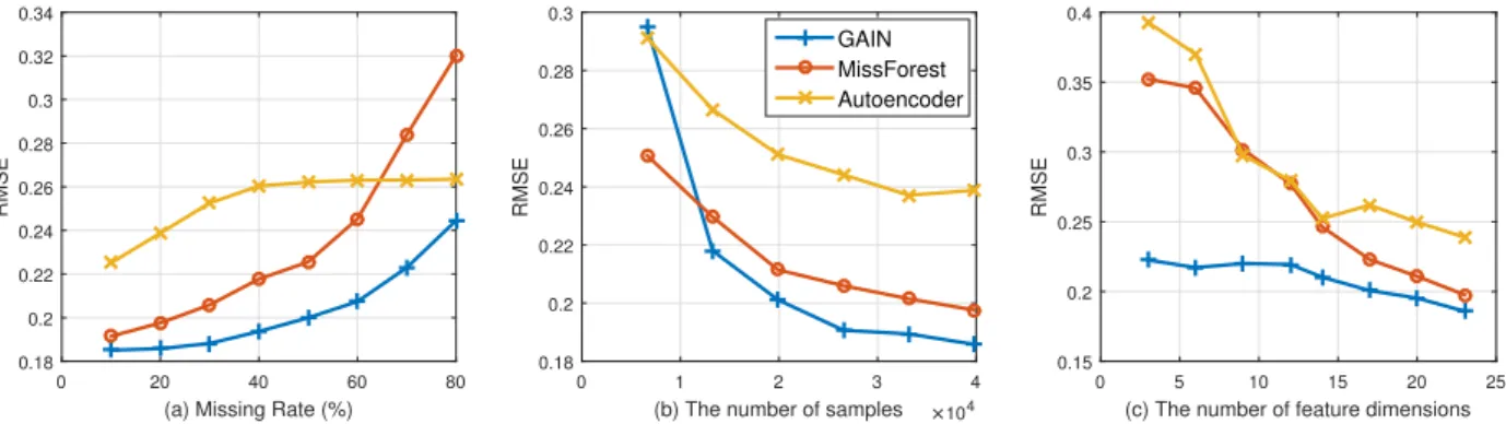
To better understand GAIN, we conduct several experiments in which we vary the missing rate, the number of samples, and the number of dimensions using Credit dataset. Fig. 2.2 shows the performance (RMSE) of GAIN within these different settings in comparison to the two most competitive benchmarks (MissForest and Auto-encoder). Fig. 2.2 (a) shows that, even though the performance of each algorithm decreases as missing rates increase, GAIN consistently outperforms the benchmarks across the entire range of missing rates.

Fig. 2.2 (b) shows that as the number of samples increases, the performance improvements of GAIN over the benchmarks also increases. This is due to the large number of parameters in GAIN that need to be optimized, however, as demonstrated on the Breast dataset (in Table 2.3), GAIN is still able to outperform the benchmarks even when the number of samples is

(46)

Algorithm Breast Spam Credit News GAIN .0546 _± .0006 .0513_± .0016 .1858 _± .0010 .1441 _± .0007 MICE .0646 _±.0028 .0699 _±.0010 .2585_± .0011 .1763 _±.0007 MissForest .0608 _±.0013 .0553 _±.0013 .1976_± .0015 .1623 _±0.012 Matrix .0946 _±.0020 .0542 _±.0006 .2602_± .0073 .2282 _±.0005 Auto-encoder .0697 _±.0018 .0670 _±.0030 .2388_± .0005 .1667 _±.0014 EM .0634 _±.0021 .0712 _±.0012 .2604_± .0015 .1912 _±.0011 Table 2.3: Imputation performance in terms of RMSE (Average _±Std of RMSE)

(a) Missing Rate (%)

0 20 40 60 80 RMSE 0.18 0.2 0.22 0.24 0.26 0.28 0.3 0.32 0.34

(b) The number of samples ×104

0 1 2 3 4 RMSE 0.18 0.2 0.22 0.24 0.26 0.28 0.3 GAIN MissForest Autoencoder

(c) The number of feature dimensions

0 5 10 15 20 25 RMSE 0.15 0.2 0.25 0.3 0.35 0.4

Figure 2.2: RMSE performance in different settings: (a) Various missing rates, (b) Various number of samples, (c) Various feature dimensions

relatively small (less than 600).

Fig. 2.2 (c) shows that GAIN is also robust to the number of feature dimensions. On the other hand, the discriminative model (MissForest) cannot as easily cope when the number of feature dimensions is small.

2.6.4 GAIN in MAR and MNAR settings

In the previous subsections, we only evaluate GAIN on MCAR setting. In this subsection, we demonstrate the outperformance of GAIN on MAR and MNAR settings as well. The following explains how we constructed datasets that satisfy MAR and MNAR settings.

Missing at random (MAR): To create an MAR dataset, we sequentially define the probability that theith component of thenth sample is observed conditional on the missingness

(47)

and values (if observed) of the previous i₋1 components to be P_im(n) = p m₍_i₎_·_N _·_e−P j<iwjmj(n)xj(n)+bj(1−mj(n)) PN l=1e −P j<iwjmj(l)xj(l)+bj(1−mj(l))

where pm₍_i_{) corresponds to the average missing rate of the}_i_{th feature, and}_w

j, bj are sampled

from _U(0,1) (but are only sampled once for the entire dataset). We sequentially sample m1, ..., md for each feature vector.

Missing not at random (MNAR): To create an MNAR dataset, we define the probability that the ith component of thenth sample is observed (Pm

i (n)) to be

P_im(n) = p

m₍_i₎_·_N _·_e−wixi(n)

PN

l=1e−wixi(l)

where againpm₍_i_{) corresponds to the average missing rate of the}_i_{th feature and}_w

i is sampled

from _U(0,1). In particular, the missingness of a data point is directly dependent on its value (with dependence determined by the weight wi).

We compare the RMSE of GAIN against other imputation algorithms on both an MAR and MNAR version of the Credit dataset. To make a fair comparison, we pass the mask matrix to all the benchmarks as an additional input so that they can also utilize the informative missingness captured by it.

Different missing rates for different features: In order to also explore the effect of different missing rates across features on the imputation performance of GAIN, we compare the MCAR, MAR and MNAR settings whenpm₍_i_{) = 0}_.₂_∀_i_{∈ {}₁_{, ..., d}_}_{(uniform) and when}

pm(i) = 0.4_×pˆm(i) where ˆpm(i)_{∼ U}(0,1) (non-uniform). The average missing rate in both cases is 0.2.

As can be seen in Table 2.4, GAIN outperforms other state-of-the-art imputation methods in all three missingness settings (both when feature missingness is uniform and non-uniform) and shows significantly better performance in the MNAR setting.

As can also be seen from the bottom side of Table 2.4, GAIN still outperforms all bench-marks in the non-uniform setting, although the performance of both GAIN and MissForest

(48)

Setting Uniform

MCAR MAR MNAR

GAIN .1858 _± .0010 .1974 _± .0006 .4046 _± .0053 MICE .2585 _± .0011 .2574 _± .0035 .5310_± .0207 MissForest .1976 _± .0015 .2194 _± .0065 .4286_± .0087 Matrix .2602 _± .0073 .2473 _± .0070 .4328_± .0036 Auto-encoder .2388 _± .0005 .2405 _± .0070 .4876_± .0097 EM .2604 _± .0015 .2755 _± .0063 .5157_± .0039 Setting Non-uniform

MCAR MAR MNAR

GAIN .2114 _± .0007 .2245 _± .0008 .4672 _± .0066 MICE .2574 _± .0014 .2344 _± .0068 .5355_± .0036 MissForest .2496 _± .0065 .2537 _± .0097 .4784_± .0102 Matrix .2356 _± .0022 .2440 _± .0122 .5216_± .0084 Auto-encoder .2444 _± .0037 .2498 _± .0129 .5017_± .0078 EM .2620 _± .0010 .3339 _± .0024 .4998_± .0053

Table 2.4: Imputation performance with uniform and non-uniform pm₍_i_{) on MCAR, MAR,}

and MNAR (Average _± Std of RMSE) settings.

(its closest competitor in the uniform setting) both decrease similarly, while MICE and Matrix completion both show improvements for the non-uniform setting.

Note that the standard deviation of the total number of missing points is higher for non-uniform pm₍_i_{) than uniform} _pm₍_i_{). As consistent with Fig. 2.2 (a), higher/lower missing}

rates yield higher/lower imputation errors; and so, due to the increased standard deviation, there is a greater variance in the performance in the non-uniform setting.

2.6.5 Prediction performance

We now compare GAIN against the same benchmarks with respect to the accuracy of post-imputation prediction. For this purpose, we use Area Under the Receiver Operating

(49)

Characteristic Curve (AUROC) as the measure of performance. To be fair to all methods, we use the same predictive model (logistic regression) in all cases. Comparisons are made on all datasets and the results are reported in Table 2.5.

Algorithm AUROC (Average ± Std)

Breast Spam Credit News

GAIN .9930 _± .0073 .9529 _± .0023 .7527 _± .0031 .9711 _± .0027 MICE .9914 _± .0034 .9495 _± .0031 .7427 _± .0026 .9451 _±.0037 MissForest .9860 _± .0112 .9520 _± .0061 .7498 _± .0047 .9597 _±.0043 Matrix .9897 _± .0042 .8639 _± .0055 .7059 _± .0150 .8578 _±.0125 Auto-encoder .9916 _± .0059 .9403 _± .0051 .7485 _± .0031 .9321 _±.0058 EM .9899 _± .0147 .9217 _± .0093 .7390 _± .0079 .8987 _±.0157

Table 2.5: Prediction performance comparison

As Table 2.5 shows, GAIN, which we have already shown to achieve the best imputation accuracy (in Table 2.3), yields the best post-imputation prediction accuracy. However, even in cases where the improvement in imputation accuracy is large, the improvements in prediction accuracy are not always significant. This is probably due to the fact that there is sufficient information in the (80%) observed data to predict the label.

Prediction accuracy with various missing rates: In this experiment, we evaluate the post-imputation prediction performance when the missing rate of the dataset is varied. Note that every dataset has their own binary label.

The results of this experiment (for GAIN and the two most competitive benchmarks) are shown in Fig. 2.3. In particular, the performance of GAIN is significantly better than the other two for higher missing rates, this is due to the fact that as the information contained in the observed data decreases (due to more values being missing), the imputation quality becomes more important, and GAIN has already been shown to provide (significantly) better quality imputations.

(50)

Missing Rate (%) 10 20 30 40 50 60 70 80 90 AUROC 0.55 0.6 0.65 0.7 0.75 0.8 GAIN Autoencoder MissForest

Figure 2.3: The AUROC performance with various missing rates with Credit dataset

2.6.6 Congeniality of GAIN

The congeniality of an imputation model is its ability to impute values th