Chapter 12
Logistic Regression
12.1 Modeling Conditional Probabilities
So far, we either looked at estimating the conditional expectations of continuous variables (as in regression), or at estimating distributions. There are many situations where however we are interested in input-output relationships, as in regression, but the output variable is discrete rather than continuous. In particular there are many situations where we have binary outcomes (it snows in Pittsburgh on a given day, or it doesn’t; this squirrel carries plague, or it doesn’t; this loan will be paid back, or it won’t; this person will get heart disease in the next five years, or they won’t). In addition to the binary outcome, we have some input variables, which may or may not be continuous. How could we model and analyze such data?
We could try to come up with a rule which guesses the binary output from the input variables. This is calledclassification, and is an important topic in statistics and machine learning. However, simply guessing “yes” or “no” is pretty crude — especially if there is no perfect rule. (Why should there be?) Something which takes noise into account, and doesn’t just give a binary answer, will often be useful. In short, we want probabilities — which means we need to fit a stochastic model.
What would be nice, in fact, would be to have conditional distribution of the responseY, given the input variables, Pr(Y|X). This would tell us about how pre-cise our predictions are. If our model says that there’s a 51% chance of snow and it doesn’t snow, that’s better than if it had said there was a 99% chance of snow (though even a 99% chance is not a sure thing). We have seen how to estimate conditional probabilities non-parametrically, and could do this using the kernels for discrete vari-ables from lecture 6. While there are a lot of merits to this approach, it does involve coming up with a model for the joint distribution of outputsY and inputsX, which can be quite time-consuming.
Let’s pick one of the classes and call it “1” and the other “0”. (It doesn’t mat-ter which is which. ThenY becomes anindicator variable, and you can convince yourself that Pr(Y=1) =E[Y]. Similarly, Pr(Y=1|X=x) = E[Y|X =x]. (In a phrase, “conditional probability is the conditional expectation of the indicator”.)
This helps us because by this point we know all about estimating conditional ex-pectations. The most straightforward thing for us to do at this point would be to pick out our favorite smoother and estimate the regression function for the indicator variable; this will be an estimate of the conditional probability function.
There are two reasons not to just plunge ahead with that idea. One is that proba-bilities must be between 0 and 1, but our smoothers will not necessarily respect that, even if all the observedyi they get are either 0 or 1. The other is that we might be better off making more use of the fact that we are trying to estimate probabilities, by more explicitly modeling the probability.
Assume that Pr(Y=1|X=x) = p(x;θ), for some function p parameterized by
θ. parameterized functionθ,andfurther assume that observations are independent of each other. The the (conditional) likelihood function is
n � i=1 Pr�Y=yi|X=xi�=�n i=1 p(xi;θ)yi(1−p(x i;θ)1−yi) (12.1)
Recall that in a sequence of Bernoulli trialsy1,...yn, where there is a constant probability of successp, the likelihood is
n
�
i=1
pyi(1−p)1−yi (12.2) As you learned in intro. stats, this likelihood is maximized whenp= ˆp=n−1�n
i=1yi.
If each trial had its own success probabilitypi, this likelihood becomes
n
�
i=1
pyi
i (1−pi)1−yi (12.3)
Without some constraints, estimating the “inhomogeneous Bernoulli” model by max-imum likelihood doesn’t work; we’d getˆpi=1 whenyi=1,ˆpi=0 whenyi=0, and learn nothing. If on the other hand we assume that the pi aren’t just arbitrary num-bers but are linked together, those constraints give non-trivial parameter estimates, and let us generalize. In the kind of model we are talking about, the constraint, pi= p(xi;θ), tells us that pi must be the same wheneverxi is the same, and ifpis a continuous function, then similar values ofxi must lead to similar values of pi. As-suming pis known (up to parameters), the likelihood is a function ofθ, and we can
estimateθby maximizing the likelihood. This lecture will be about this approach.
12.2 Logistic Regression
To sum up: we have a binary output variableY, and we want to model the condi-tional probability Pr(Y=1|X =x)as a function ofx; any unknown parameters in the function are to be estimated by maximum likelihood. By now, it will not surprise you to learn that statisticians have approach this problem by asking themselves “how can we use linear regression to solve this?”
12.2. LOGISTIC REGRESSION 225 1. The most obvious idea is to let p(x)be a linear function ofx. Every increment of a component ofxwould add or subtract so much to the probability. The conceptual problem here is that pmust be between 0 and 1, and linear func-tions are unbounded. Moreover, in many situafunc-tions we empirically see “dimin-ishing returns” — changingpby the same amount requires a bigger change in xwhenpis already large (or small) than when pis close to 1/2. Linear models can’t do this.
2. The next most obvious idea is to let logp(x)be a linear function ofx, so that changing an input variablemultipliesthe probability by a fixed amount. The problem is that logarithms are unbounded in only one direction, and linear functions are not.
3. Finally, the easiest modification of logpwhich has an unbounded range is the logistic(or logit) transformation, log1−pp. We can makethisa linear func-tion ofxwithout fear of nonsensical results. (Of course the results could still happen to bewrong, but they’re notguaranteedto be wrong.)
This last alternative islogistic regression.
Formally, the model logistic regression model is that log p(x)
1−p(x)=β0+x·β (12.4)
Solving for p, this gives
p(x;b,w) = e
β0+x·β
1+eβ0+x·β =
1
1+e−(β0+x·β) (12.5)
Notice that the over-all specification is a lot easier to grasp in terms of the transformed probability that in terms of the untransformed probability.1
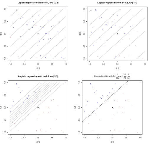
To minimize the mis-classification rate, we should predictY =1 when p≥0.5 andY=0 whenp<0.5. This means guessing 1 wheneverβ0+x·βis non-negative, and 0 otherwise. So logistic regression gives us a linear classifier. The decision boundary separating the two predicted classes is the solution of β0+x·β = 0,
which is a point ifxis one dimensional, a line if it is two dimensional, etc. One can show (exercise!) that the distance from the decision boundary isβ0/�β�+x·β/�β�.
Logistic regression not only says where the boundary between the classes is, but also says (via Eq. 12.5) that the class probabilities depend on distance from the boundary, in a particular way, and that they go towards the extremes (0 and 1) more rapidly when �β� is larger. It’s these statements about probabilities which make logistic regression more than just a classifier. It makes stronger, more detailed predictions, and can be fit in a different way; but those strong predictions could be wrong.
Using logistic regression to predict class probabilities is amodeling choice, just like it’s a modeling choice to predict quantitative variables with linear regression.
1Unless you’ve taken statistical mechanics, in which case you recognize that this is the Boltzmann
-+ -++ + - + -+ + + + - -+ + -+ + + -+ -+ + -- + + - + + -+ + -+ + -+ - + -+ -+ -1.0 -0.5 0.0 0.5 1.0 -1.0 -0.5 0.0 0.5 1.0
Logistic regression with b=-0.1, w=(-.2,.2)
x[,1] x[,2] -+ + ++ + + -+ + -- -+ -+ -+ -+ + + - -+ + -+ -+ + -+ -+ + --1.0 -0.5 0.0 0.5 1.0 -1.0 -0.5 0.0 0.5 1.0
Logistic regression with b=-0.5, w=(-1,1)
x[,1] x[,2] -+ - -+ + -+ -+ + -+ -+ + -- -- -+ + -+ + + -+ -+ + --1.0 -0.5 0.0 0.5 1.0 -1.0 -0.5 0.0 0.5 1.0
Logistic regression with b=-2.5, w=(-5,5)
x[,1] x[,2] -+ - -+ + -+ -+ + -+ -+ + -- -+ - -+ + -+ + -+ -+ + --1.0 -0.5 0.0 0.5 1.0 -1.0 -0.5 0.0 0.5 1.0
Linear classifier with b=1
2 2,w= ! ! !!1 2, 1 2 ! ! ! x[,1] x[,2]
Figure 12.1: Effects of scaling logistic regression parameters. Values ofx1andx2are the same in all plots (∼Unif(−1,1)for both coordinates), but labels were generated randomly from logistic regressions withβ0=−0.1,β= (−0.2,0.2)(top left); from
β0=−0.5,β= (−1,1)(top right); fromβ0=−2.5,β= (−5,5)(bottom left); and
from a perfect linear classifier with the same boundary. The large black dot is the origin.
12.2. LOGISTIC REGRESSION 227 In neither case is the appropriateness of the model guaranteed by the gods, nature, mathematical necessity, etc. We begin by positing the model, to get something to work with, and we end (if we know what we’re doing) by checking whether it really does match the data, or whether it has systematic flaws.
Logistic regression is one of the most commonly used tools for applied statistics and discrete data analysis. There are basically four reasons for this.
1. Tradition.
2. In addition to the heuristic approach above, the quantity logp/(1−p)plays an important role in the analysis of contingency tables (the “log odds”). Classi-fication is a bit like having a contingency table with two columns (classes) and infinitely many rows (values ofx). With a finite contingency table, we can es-timate the log-odds for each row empirically, by just taking counts in the table. With infinitely many rows, we need some sort of interpolation scheme; logistic regression is linear interpolation for the log-odds.
3. It’s closely related to “exponential family” distributions, where the probabil-ity of some vectorv is proportional to expβ0+�mj=1fj(v)βj. If one of the
components ofv is binary, and the functions fj are all the identity function, then we get a logistic regression. Exponential families arise in many contexts in statistical theory (and in physics!), so there are lots of problems which can be turned into logistic regression.
4. It often works surprisingly well as a classifier. But, many simple techniques of-ten work surprisingly well as classifiers, and this doesn’t really testify to logistic regression getting the probabilities right.
12.2.1 Likelihood Function for Logistic Regression
Because logistic regression predicts probabilities, rather than just classes, we can fit it using likelihood. For each training data-point, we have a vector of features, xi, and an observed class,yi. The probability of that class was either p, ifyi=1, or 1−p, if yi=0. The likelihood is then
L(β0,β) = n � i=1 p(xi)yi(1−p(x i)1−yi (12.6)
(I could substitute in the actual equation forp, but things will be clearer in a moment if I don’t.) The log-likelihood turns products into sums:
�(β0,β) = n � i=1 yilogp(xi) + (1−yi)log1−p(xi) (12.7) = n � i=1 log1−p(xi) + n � i=1 yilog p(xi) 1−p(xi) (12.8) = n � i=1 log1−p(xi) + n � i=1 yi(β0+xi·β) (12.9) = n � i=1 −log1+eβ0+xi·β+ n � i=1 yi(β0+xi·β) (12.10)
where in the next-to-last step we finally use equation 12.4.
Typically, to find the maximum likelihood estimates we’d differentiate the log likelihood with respect to the parameters, set the derivatives equal to zero, and solve. To start that, take the derivative with respect to one component ofβ, sayβj.
∂ � ∂ βj = − n � i=1 1 1+eβ0+xi·βe β0+xi·βx i j+ n � i=1 yixi j (12.11) = n � i=1 �y i−p(xi;β0,β)�xi j (12.12)
We are not going to be able to set this to zero and solve exactly. (That’s a transcenden-tal equation, and there is no closed-form solution.) We can however approximately solve it numerically.
12.2.2 Logistic Regression with More Than Two Classes
IfY can take on more than two values, sayk of them, we can still use logistic regres-sion. Instead of having one set of parametersβ0,β, each classcin 0 :(k−1)will have
its own offsetβ(0c)and vectorβ(c), and the predicted conditional probabilities will be
Pr�Y=c|X� =x�= eβ (c) 0+x·β(c) � ceβ (c) 0+x·β(c) (12.13) You can check that when there are only two classes (say, 0 and 1), equation 12.13 reduces to equation 12.5, withβ0=β(01)−β(
0)
0 andβ=β(1)−β(0). In fact, no matter
how many classes there are, we can always pick one of them, sayc=0, and fix its parameters at exactly zero, without any loss of generality2.
2Since we can arbitrarily chose which class’s parameters to “zero out” without affecting the predicted
probabilities, strictly speaking the model in Eq. 12.13 isunidentified. That is, different parameter settings
lead toexactlythe same outcome, so we can’t use the data to tell which one is right. The usual response
here is to deal with this by a convention: wedecideto zero out the parameters of the first class, and then
12.3. NEWTON’S METHOD FOR NUMERICAL OPTIMIZATION 229 Calculation of the likelihood now proceeds as before (only with more book-keeping), and so does maximum likelihood estimation.
12.3 Newton’s Method for Numerical Optimization
There are a huge number of methods for numerical optimization; we can’t cover all bases, and there is no magical method which will always work better than anything else. However, there are some methods which work very well on an awful lot of the problems which keep coming up, and it’s worth spending a moment to sketch how they work. One of the most ancient yet important of them is Newton’s method (alias “Newton-Raphson”).Let’s start with the simplest case of minimizing a function of one scalar variable, say f(β). We want to find the location of the global minimum,β∗. We suppose that f is smooth, and thatβ∗is a regular interior minimum, meaning that the derivative
atβ∗is zero and the second derivative is positive. Near the minimum we could make
a Taylor expansion: f(β)≈f(β∗) +12(β−β∗)2 d 2f dβ2 �� �� � β=β∗ (12.14) (We can see here that the second derivative has to be positive to ensure that f(β)>
f(β∗).) In words, f(β)is close to quadratic near the minimum.
Newton’s method uses this fact, and minimizes a quadraticapproximationto the function we are really interested in. (In other words, Newton’s method is to replace the problem we want to solve, with a problem which wecansolve.) Guessan ini-tial pointβ(0). If this is close to the minimum, we can take a second order Taylor
expansion aroundβ(0)and it will still be accurate:
f(β)≈f(β(0)) + (β−β(0))d f d w �� �� � β=β(0) +12�β−β(0)�2 d2f d w2 �� �� � β=β(0) (12.15) Now it’s easy to minimize the right-hand side of equation 12.15. Let’s abbreviate the derivatives, because they get tiresome to keep writing out: d wd f���
β=β(0)= f
�(β(0)),
d2f
d w2���
β=β(0) =f
��(β(0)). We just take the derivative with respect toβ, and set it equal
to zero at a point we’ll callβ(1):
0 = f�(β(0)) +1
2f��(β(
0))2(β(1)−β(0)) (12.16)
β(1) = β(0)− f�(β(0))
f��(β(0)) (12.17)
The valueβ(1)should be a better guess at the minimumβ∗than the initial oneβ(0)
was. So if we useitto make a quadratic approximation to f, we’ll get a better ap-proximation, and so we caniteratethis procedure, minimizing one approximation
and then using that to get a new approximation:
β(n+1)=β(n)− f�(β(n))
f��(β(n)) (12.18)
Notice that the true minimumβ∗is afixed pointof equation 12.18: if we happen to land on it, we’ll stay there (since f�(β∗) =0). We won’t show it, but it can be proved
thatifβ(0)is close enough toβ∗, thenβ(n)→β∗, and that in general|β(n)−β∗|=
O(n−2), a very rapid rate of convergence. (Doubling the number of iterations we use
doesn’t reduce the error by a factor of two, but by a factor of four.) Let’s put this together in an algorithm.
my.newton = function(f,f.prime,f.prime2,beta0,tolerance=1e-3,max.iter=50) { beta = beta0
old.f = f(beta) iterations = 0 made.changes = TRUE
while(made.changes & (iterations < max.iter)) { iterations <- iterations +1
made.changes <- FALSE
new.beta = beta - f.prime(beta)/f.prime2(beta) new.f = f(new.beta)
relative.change = abs(new.f - old.f)/old.f -1 made.changes = (relative.changes > tolerance) beta = new.beta
old.f = new.f }
if (made.changes) {
warning("Newton’s method terminated before convergence") }
return(list(minimum=beta,value=f(beta),deriv=f.prime(beta), deriv2=f.prime2(beta),iterations=iterations, converged=!made.changes))
}
The first three arguments here have to all befunctions. The fourth argument is our initial guess for the minimum,β(0). The last arguments keep Newton’s method from
cycling forever: tolerancetells it to stop when the function stops changing very much (the relative difference betweenf(β(n))andf(β(n+1))is small), andmax.iter
tells it to never do more than a certain number of steps no matter what. The return value includes the estmated minimum, the value of the function there, and some diagnostics — the derivative should be very small, the second derivative should be positive, etc.
You may have noticed some potential problems — what if we land on a point where f��is zero? What if f(β(n+1))> f(β(n))? Etc. There are ways of handling
these issues, and more, which are incorporated into real optimization algorithms from numerical analysis — such as theoptimfunction in R; I strongly recommend
12.3. NEWTON’S METHOD FOR NUMERICAL OPTIMIZATION 231 you use that, or something like that, rather than trying to roll your own optimization code.3
12.3.1 Newton’s Method in More than One Dimension
Suppose that the objective f is a function of multiple arguments, f(β1,β2,...βp).
Let’s bundle the parameters into a single vector,w. Then the Newton update is
β(n+1)=β(n)−H−1(β(n))∇f(β(n)) (12.19)
where∇f is thegradientoff, its vector of partial derivatives[∂ f/∂ β1,∂ f/∂ β2,...∂ f/∂ βp],
andHis theHessianoff, its matrix of second partial derivatives,Hi j=∂2f/∂ βi∂ βj.
CalculatingH and∇f isn’t usually very time-consuming, but taking the inverse ofHis, unless it happens to be a diagonal matrix. This leads to variousquasi-Newton methods, which either approximateHby a diagonal matrix, or take a proper inverse ofHonly rarely (maybe just once), and then try to update an estimate ofH−1(β(n))
asβ(n)changes.
12.3.2 Iteratively Re-Weighted Least Squares
This discussion of Newton’s method is quite general, and therefore abstract. In the particular case of logistic regression, we can make everything look much more “sta-tistical”.
Logistic regression, after all, is a linear model for a transformation of the proba-bility. Let’s call this transformationg:
g(p)≡log p
1−p (12.20)
So the model is
g(p) =β0+x·β (12.21)
andY|X =x∼Bi nom(1,g−1(β
0+x·β)). It seems that what we should want to
do is take g(y)and regress it linearly on x. Of course, the variance ofY, according to the model, is going to chance depending onx— it will be(g−1(β
0+x·β))(1−
g−1(β
0+x·β))— so we really ought to do a weighted linear regression, with weights
inversely proportional to that variance. Since writingβ0+x·βis getting annoying, let’s abbreviate it byµ(for “mean”), and let’s abbreviate that variance asV(µ).
The problem is thatyis either 0 or 1, sog(y)is either−∞or+∞. We will evade this by using Taylor expansion.
g(y)≈g(µ) + (y−µ)g�(µ)≡z (12.22)
The right hand side, zwill be oureffectiveresponse variable. To regress it, we need its variance, which by propagation of error will be(g�(µ))2V(µ).
3optimactually is a wrapper for several different optimization methods;method=BFGSselects a
Notice that both the weights and z depend on the parameters of our logistic regression, throughµ. So having done this once, we should really use the new
pa-rameters to updatezand the weights, and do it again. Eventually, we come to a fixed point, where the parameter estimates no longer change.
The treatment above is rather heuristic4, but it turns out to be equivalent to using
Newton’s method, with the expected second derivative of the log likelihood, instead of its actual value.5 Since, with a large number of observations, the observed
sec-ond derivative should be close to the expected secsec-ond derivative, this is only a small approximation.
12.4 Generalized Linear Models and Generalized
Ad-ditive Models
Logistic regression is part of a broader family ofgeneralized linear models(GLMs), where the conditional distribution of the response falls in some parametric family, and the parameters are set by the linear predictor. Ordinary, least-squares regression is the case where response is Gaussian, with mean equal to the linear predictor, and constant variance. Logistic regression is the case where the response is binomial, with nequal to the number of data-points with the givenx(often but not always 1), andp is given by Equation 12.5. Changing the relationship between the parameters and the linear predictor is called changing thelink function. For computational reasons, the link function is actually the function you apply to the mean response to get back the linear predictor, rather than the other way around — (12.4) rather than (12.5). There are thus other forms of binomial regression besides logistic regression.6 There is also
Poisson regression (appropriate when the data are counts without any upper limit), gamma regression, etc.; we will say more about these in Chapter 13.
In R, any standard GLM can be fit using the (base) glmfunction, whose
syn-tax is very similar to that oflm. The major wrinkle is that, of course, you need
to specify the family of probability distributions to use, by thefamilyoption —
family=binomialdefaults to logistic regression. (Seehelp(glm)for the gory
details on how to do, say, probit regression.) All of these are fit by the same sort of numerical likelihood maximization.
One caution about using maximum likelihood to fit logistic regression is that it can seem to work badly when the training datacanbe linearly separated. The reason is that, to make the likelihood large,p(xi)should be large whenyi=1, andpshould be small whenyi =0. Ifβ0,β0is a set of parameters which perfectly classifies the
training data, thencβ0,cβis too, for anyc>1, but in a logistic regression the second
4That is, mathematically incorrect.
5This takes a reasonable amount of algebra to show, so we’ll skip it. The key point however is the
following. Take a single Bernoulli observation with success probabilityp. The log-likelihood isYlogp+
(1−Y)log1−p. The first derivative with respect topisY/p−(1−Y)/(1−p), and the second derivative
is−Y/p2−(1−Y)/(1−p)2. Taking expectations of the second derivative gives−1/p−1/(1−p) =
−1/p(1−p). In other words,V(p) =−1/E�����. Using weights inversely proportional to the variance
thus turns out to be equivalent to dividing by the expected second derivative.
6My experience is that these tend to give similar error rates as classifiers, but have rather different
12.4. GENERALIZED LINEAR MODELS AND GENERALIZED ADDITIVE MODELS233 set of parameters will have more extreme probabilities, and so a higher likelihood.
For linearly separable data, then, there is no parameter vector whichmaximizesthe likelihood, since�can always be increased by making the vector larger but keeping
it pointed in the same direction.
You should, of course, be so lucky as to have this problem.
12.4.1 Generalized Additive Models
A natural step beyond generalized linear models is generalized additive models (GAMs), where instead of making the transformed mean response alinearfunction of the inputs, we make it anadditivefunction of the inputs. This means combining a function for fitting additive models with likelihood maximization. The R function here isgam, from the CRAN package of the same name. (Alternately, use the func-tiongamin the packagemgcv, which is part of the default R installation.) We will look at how this works in some detail in Chapter 13.
GAMs can be used to check GLMs in much the same way that smoothers can be used to check parametric regressions: fit a GAM and a GLM to the same data, then simulate from the GLM, and re-fit both models to the simulated data. Repeated many times, this gives a distribution for how much better the GAM will seem to fit than the GLM does,even when the GLM is true. You can then read a p-value off of this distribution.
12.4.2 An Example (Including Model Checking)
Here’s a worked R example, using the data from the upper right panel of Figure 12.1. The 50×2 matrixxholds the input variables (the coordinates are independently and uniformly distributed on[−1,1]), andy.1the corresponding class labels, themselves generated from a logistic regression withβ0=−0.5,β= (−1,1).
> logr = glm(y.1 ~ x[,1] + x[,2], family=binomial) > logr
Call: glm(formula = y.1 ~ x[, 1] + x[, 2], family = binomial)
Coefficients:
(Intercept) x[, 1] x[, 2]
-0.410 -1.050 1.366
Degrees of Freedom: 49 Total (i.e. Null); 47 Residual
Null Deviance: 68.59
Residual Deviance: 58.81 AIC: 64.81
> sum(ifelse(logr$fitted.values<0.5,0,1) != y.1)/length(y.1) [1] 0.32
Thedevianceof a model fitted by maximum likelihood is (twice) the difference between its log likelihood and the maximum log likelihood for asaturatedmodel, i.e., a model with one parameter per observation. Hopefully, the saturated model
can give a perfect fit.7 Here the saturated model would assign probability 1 to the
observed outcomes8, and the logarithm of 1 is zero, so D = 2�(β�
0,β�). The null
deviance is what’s achievable by using just a constant biasb and settingw=0. The fitted model definitely improves on that.9
The fitted values of the logistic regression are the class probabilities; this shows that the error rate of the logistic regression, if you force it to predict actual classes, is 32%. This sounds bad, but notice from the contour lines in the figure that lots of the probabilities are near 0.5, meaning that the classes are just genuinely hard to predict. To see how well the logistic regression assumption holds up, let’s compare this to a GAM.10
> library(gam)
> gam.1 = gam(y.1~lo(x[,1])+lo(x[,2]),family="binomial") > gam.1
Call:
gam(formula = y.1 ~ lo(x[, 1]) + lo(x[, 2]), family = "binomial") Degrees of Freedom: 49 total; 41.39957 Residual
Residual Deviance: 49.17522
This fits a GAM to the same data, using lowess smoothing of both input variables. Notice that the residual deviance is lower. That is, the GAM fits better. We expect this; the question is whether the difference is significant, or within the range of what we should expect when logistic regression is valid. To test this, we need to simulate from the logistic regression model.
simulate.from.logr = function(x, coefs) {
require(faraway) # For accessible logit and inverse-logit functions n = nrow(x)
linear.part = coefs[1] + x %*% coefs[-1] probs = ilogit(linear.part) # Inverse logit y = rbinom(n,size=1,prob=probs)
return(y) }
Now we simulate from our fitted model, and re-fit both the logistic regression and the GAM.
7The factor of two is so that the deviance will have aχ2distribution. Specifically, if the model withp
parameters is right, the deviance will have aχ2distribution withn−pdegrees of freedom.
8This is not possible when there are multiple observations with the same input features, but different
classes.
9AIC is of course the Akaike information criterion,−2�+2q, withqbeing the number of parameters
(here,q=3). AIC has some truly devoted adherents, especially among non-statisticians, but I have been
deliberately ignoring it and will continue to do so. Basically, to the extent AIC succeeds, it works as fast, large-sample approximation to doing leave-one-out cross-validation. Claeskens and Hjort (2008) is a thorough, modern treatment of AIC and related model-selection criteria from a statistical viewpoint.
10Previous examples of using GAMs have mostly used themgcvpackage and spline smoothing. There
is no particular reason to switch to thegamlibrary and lowess smoothing here, but there’s also no real
12.4. GENERALIZED LINEAR MODELS AND GENERALIZED ADDITIVE MODELS235
delta.deviance.sim = function (x,logistic.model) {
y.new = simulate.from.logr(x,logistic.model$coefficients)
GLM.dev = glm(y.new ~ x[,1] + x[,2], family="binomial")$deviance
GAM.dev = gam(y.new ~ lo(x[,1]) + lo(x[,2]), family="binomial")$deviance return(GLM.dev - GAM.dev)
}
Notice that in this simulation we are not generating newX� values. The logistic
re-gression and the GAM are both models for the responseconditionalon the inputs, and are agnostic about how the inputs are distributed, or even whether it’s meaning-ful to talk about their distribution.
Finally, we repeat the simulation a bunch of times, and see where the observed difference in deviances falls in the sampling distribution.
> delta.dev = replicate(1000,delta.deviance.sim(x,logr)) > delta.dev.observed = logr$deviance - gam.1$deviance # 9.64 > sum(delta.dev.observed > delta.dev)/1000
[1] 0.685
In other words, the amount by which a GAM fits the data better than logistic regres-sion is pretty near the middle of the null distribution. Since the example data really didcome from a logistic regression, this is a relief.
0 10 20 30 0.00 0.02 0.04 0.06 0.08 0.10
Amount by which GAM fits better than logistic regression
Sampling distribution under logistic regression
N = 1000 Bandwidth = 0.8386
Density
Figure 12.2: Sampling distribution for the difference in deviance between a GAM and a logistic regression, on data generated from a logistic regression. The observed difference in deviances is shown by the dashed horizontal line.
12.5. EXERCISES 237
12.5 Exercises
To think through, not to hand in.
1. A multiclass logistic regression, as in Eq. 12.13, has parametersβ(0c)andβ(c)
for each classc. Show that we can always get the same predicted probabilities by settingβ(0c)=0,β(c) =0 for any one classc, and adjusting the parameters
for the other classes appropriately.
2. Find the first and second derivatives of the log-likelihood for logistic regression with one predictor variable. Explicitly write out the formula for doing one step of Newton’s method. Explain how this relates to re-weighted least squares.