Objective Risk Evaluation for Automated Security
Management
Mohammad Salim Ahmed•Ehab Al-Shaer•
Mohamed Taibah•Latifur Khan
Received: 12 February 2009 / Accepted: 16 September 2010 / Published online: 30 October 2010 ÓSpringer Science+Business Media, LLC 2010
Abstract Network security depends on a number of factors. And a common characteristic of these factors is that they are dynamic in nature. Such factors include new vulnerabilities and threats, the network policy structure and traffic. These factors can be divided into two broad categories. Network risk and service risk. As the name implies, the former one corresponds to risk associated with the network policy whereas the later one depends on the services and software running on the system. Therefore, evaluating security from both the service and policy perspective can allow the management system to make decisions regarding how a system should be changed to enhance security as par the management objective. Such decision making includes choosing between alternative security architectures, designing security countermeasures, and to systematically modify security config-urations to improve security. As there may be real time changes to the network threat, this evaluation must be done dynamically to handle such changes. In this paper, we provide a security metric framework that quantifies objectively the most significant security risk factors, which include existing vulnerabilities, historical trend of vulnerabilities of the remotely accessible services, prediction of potential vulnerabilities for these services and their estimated severity, unused address space
M. S. Ahmed (&)L. Khan
University of Texas at Dallas, Richardson, TX 75080, USA e-mail: [email protected]
L. Khan
e-mail: [email protected] E. Al-Shaer
University of North Carolina Charlotte, Charlotte, NC 28223, USA e-mail: [email protected]
M. Taibah
DePaul University, Chicago, IL 60604, USA e-mail: [email protected]
and finally propagation of an attack within the network. These factors cover both the service aspect and the network aspect of risk toward a system. We have imple-mented this framework as a user-friendly tool calledRisk based prOactive seCurity cOnfiguration maNAger (ROCONA)and showed how this tool simplifies security configuration management of services and policies in a system using risk mea-surement and mitigation. We also combine all the components into one single metric and present validation experiments using real-life vulnerability data from
National Vulnerability Database (NVD) and show comparison with two existing risk measurement tools.
Keywords Security evaluationRisk prediction Vulnerability measure Attack propagationAttack immunityQuality of protection
1 Introduction
In order to formulate a security management framework, it is imperative that we have a security measurement scheme with which we can compare different network security policies. And, to measure security, we have to first decide on how we should consider a computer network. Acomputer network systemcan be visualized from both physical and security perspectives. From a physical perspective, such a
systemcan be considered as consisting of a number of computers, servers and other system components interconnected via high speed LAN or WAN. However, when the samesystemis visualized from a security perspective, it can be divided into its
service and network part. In this paper, we have formulated our security measurement and management framework using this security perspective.
The network part of a computer network system allows data to come into the system, some of which may be generated with the intent of an attack and are malicious in nature and some, on the other hand, are benign for the system. After such malicious data makes its way into the system, its impact depends on which services or software in the system are affected by it. Therefore, following this notion, asystemcan be considered as a combination of multiple services that interact with each other and also with other network systems using its network communication.
Since, we can model a system in such a way, risk evaluation of individual services can help in identifying services that pose higher risk. This in turn, allows the system administrators to pay extra attention to such services. We can then incorporate this information in our network security policy or access options to enhance security. In this paper, network security policy is defined as a set of objectives, rules of behavior for users and administrators, list of active services and corresponding software and finally, requirements for system configuration and management. Therefore, it also specifies which services are part of the system. But, meaningful changes to security policy can only happen if we have a security measure of all the services. If the risk of a single service can be quantified, then existing aggregating methods can be used to evaluate the security of all the services in a system. Along with the service risk measurement, integrating it with the network/policy risk measurement can provide a complete risk analysis of the
system. This can allow the management to employ resources for risk mitigation based on the severity and importance of each of these two aspects of risk.
The effectiveness of a security metric depends on the security measurement techniques and tools that enable network administrators to analyze and evaluate network security. Our proposed new framework and user-friendly implementation for network security evaluation can quantitatively measure the security of a network based on these two critical risk aspects - the risk of having a successful attack due to the services and the risk of this attack being propagated within the network due to the policy. Finally all these components are integrated into a single metric called
Quality of Protection Metric (QoPM) to portray the overall security level of the network for the decision makers.
We have a number of contributions in this paper. First, our proposed tool, based on our framework, can help in comparing services and security policies with each other to determine which ones are more secure. It is also possible to judge the effect of a change to the policy by comparing the security metrics before and after the change. And, this comparison can be done, in aggregated form (e.g., weighted average) or component wise, based on user needs. Second, our framework and its implemen-tation is also an important step towardadaptive security systems, in which, networks can be evaluated and automatically hardened accordingly by constantly monitoring changes in the network and service vulnerabilities. We used the Java Programming Language to implement the proposed metrics in one graphical user-interface called
ROCONA. This tool simplifies periodic risk measurement and management. Third, the underlying framework of our tool is more advanced with respect to the existing tools and previous research works. Previous research include those that scan or analyze a given network to find out allowed traffic patterns and vulnerabilities in the services. However, most of them do not predict the future state of the security of the network, consider the policy immunity or spurious risk. Research that do try to predict future vulnerabilities like [1] is limited to predicting software bugs and it requires inside knowledge of the studied software. In this respect, our prediction model is general and can work using only publicly available data. Finally, using the
National Vulnerability Database published by NIST [2], we performed extensive evaluation of our proposed model. The results show high level of accuracy in the evaluation and a new direction towards security measurement.
The organization of the paper is as follows. First, a detailed description of the entire framework is given in Sect.2 followed by our implementation of the framework, deployment and a case study in Sect.3. Then, we present our strategy of combining all the scores in Sect.4, followed by our experiments, results and discussion on the experimental results in Sect.5. Next, we discuss the related works in Sect.6. And finally, we present our conclusion and some directions of future research in Sect.7.
2 Security Risk Evaluation Framework
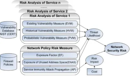
As can be seen from Fig.1, we have modeled our framework as a combination of two parts. The first part measures the security level of the services within the computer network system based on vulnerability analysis. This analysis considers the presence
of existing vulnerabilities, the dormant risk based on previous vulnerabilities and the potential future risk. In the second part, the service exposure to outside network by filtering policies, the degree of penetration or impact of successful attacks against the network and the risk due to traffic destined for unused address space are measured from a network security policy perspective. The three service risk components, the exposure factor and the unused address space exposure, together give us the threat likelihood and at the same time the attack propagation provides us with the risk impact to the network of interest. When the risk impact is combined with the cost of the damage, we get the contribution of network policies in the total risk. In this paper, we use the terms vulnerability and risk interchangeably. If a service has vulnerabilities, we consider it as posing a risk towards the corresponding system. Also, the terms security and risk are regarded as opposites. Therefore, when we consider security, high values indicate high level of security and low values indicate low security. On the other hand, when we use the term vulnerability, high values indicate high vulnerability or risk (i.e., low security) and vice versa. Also, we shall refer to acomputer network system(with both its service and network part) simply as asystemfrom this point forward.
2.1 Service Risk Measurement
In this section, we describe and discuss in detail the calculation method of our vulnerability analysis for service risk measurement. This analysis comprises of
Historical Vulnerability Measure,Probabilistic Vulnerability MeasureandExisting Vulnerability Measure.
2.1.1 Historical Vulnerability Measure
Using the vulnerability history of a service, the Historical Vulnerability Measure (HVM) quantifies how vulnerability prone a given service has been in the past. Considering both the frequency and age of the vulnerabilities, we combine the
severity scores of past vulnerabilities so that a service with a high frequency of vulnerabilities in the near past has a highHVM.
Let the set of services in the system beS. We divide the set of vulnerabilities
HV(si) of each service si[ Sinto three groups—HVH(si),HVM(si) and HVL(si) for
vulnerabilities that pose high, medium and low risks to the system. In evaluating a service, the vulnerabilities discovered a long time ago should carry smaller weight, because with time these would be analyzed, understood and patched. And our analysis of vulnerabilities found the service vulnerability to be less dependent on past vulnerabilities. So, we regard the relationship between a vulnerability and its age as nonlinear and we apply an exponential decay function of the age of the vulnerability. The age of a vulnerability indicates how much time has passed since its discovery and is measured in number of days. The parameter b in the decay function controls how fast the factor decays with age. In computing theHVM of individual services, we sum up the decayed scores in each class, and take their weighted sum. Finally, we take its natural logarithm to bring it to a more manageable magnitude. Before taking the logarithm, we add 1 to the sum so that a sum of 0 will not result in?, and the result is always positive. TheHVMof service
si,HVM(si) is calculated as follows: HVMðsiÞ ¼ln 1þ X X2fH;M;Lg wX: X vj2HVXðsiÞ SSðvjÞ:ebAgeðvjÞ 0 @ 1 A ð1Þ
In this equation,vjis a vulnerability of servicesi,Age(vj) can have a range of (0,
?) and SS(vj) is its severity. Finally, the Aggregate Historical Vulnerability
Measureof the whole system,AHVM(S), is calculated as
AHVMðSÞ ¼ln X si2S
eHVMðsiÞ !
ð2Þ This equation is designed to be dominated by the highestHVM of the services exposed by the policy. We take the exponential average of all theHVMs so that the
AHVMscore will be at least equal to the highestHVM, and will increase with the
HVM’s of the other services. If arithmetic average was taken, then the risk of the most vulnerable services would have been undermined. Our formalization using the exponential average is validated through our conducted experiments.
2.1.2 Probabilistic Vulnerability Measure
The Probabilistic Vulnerability Measure (PVM) combines the probability of a vulnerability being discovered in the next period of time and the expected severity of that vulnerability. This measure, therefore, gives an indication of the risk faced by the system in the future.
Using the vulnerability history of a service, we can calculate the probability of at least one new vulnerability being published in a given period of time. From the vulnerability history, we can also compute theExpected Severity of the predicted vulnerabilities.
We calculateExpected Risk (ER)for a service as the product of the probability of at least one new vulnerability affecting the service in the next period of time and the expected severity of the vulnerabilities. We can compare two services using this measure—a higher value of the measure will indicate a higher chance of that service being vulnerable in the near future.
For each service, we construct a list of the interarrival times between each pair of consecutive vulnerabilities published for that service. Then we compute the probability of the interarrival time being less than or equal to a given period of time,
T. LetPsibe the probability thatdsi, the number of days before the next vulnerability
of the servicesiis exposed, is less than or equal to a given time interval,T, i.e.,
Psi ¼P dð siTÞ ð3Þ
To compute the expected severity, first we build the probability distribution of the severities of the vulnerabilities affecting the service in the past. LetX be the random variable corresponding to the severities, andx1,x2, ... be the values taken byX. Then, the expectation ofXsi for servicesiis given by (4):
E½Xsi ¼ X1
i¼1;xj2si
xjPðxjÞ ð4Þ
whereP(xj) is the probability that a vulnerability with severityxjoccurs for service
si. Finally, we can define the Expected Risk (ER), of a service sias follows.
ERðsiÞ ¼PsiE½Xsi ð5Þ
IfSis the set of services exposed by the policy, we can combine the probabilities of all the services exposed by the policy to compute thePVMof the system as in (6).
PVM Sð Þ ¼lnX si2S
eERðsiÞ ð6Þ
For combining the expected risks into one single measure, we are using the exponential average method like theAHVM, so that thePVMof a system is at least as high as the highest expected risk of a service in the system. Therefore, from definition perspective,PVMis similar to AHVMas both measures correspond to a collection of services whereas HVM and ER are similar as they correspond to a single service.
In order to calculatePVM, we have looked into different methods to model the interarrival times. The first method that we have analyzed is Exponential Distribution. Interarrival times usually follow exponential distribution [3]. In order to evaluate (3) for a given service, we can fit the interarrival times to an exponential distribution, and we can then find the required probability from the Cumulative Distribution Function (CDF). Ifkis the mean interarrival time of servicesi, then the
interarrival times of service si, dsi, will be distributed exponentially with the
following CDF:
Psi ¼P dð siTÞ ¼Fdsið Þ ¼T 1e
The next method that have been analyzed is Empirical Distribution. We can model the distribution of the interarrival times of the data using empirical distribution. The frequency distribution is used to construct aCDFfor this purpose.
In this case, the empiricalCDFof the interarrival time,dsi, will be: Psi ¼P dð siTÞ ¼Fdsið Þ ¼T P xTfið Þx Pf ið Þx ð8Þ Finally, exponential smoothing, aTime Series Analysistechnique was also used for identifying the underlying trend of the data and finding the probabilities.
2.1.3 Existing Vulnerability Measure
Existing vulnerability is important as sometimes the services in the system are left unpatched or, in cases where there are no known patches available. Also, when a vulnerability is discovered, it takes time before a patch is introduced for it. During that time, the network and services are vulnerable to outside attack. TheExisting Vulnerability Measure (EVM) measures this risk. EVM has been studied and formalized in our previous work [4].
We again use theexponential averageto quantify the worst case scenario so that the score is always at least as great as the maximum vulnerability value in the data. LetEV(S) be the set of vulnerabilities that currently exist in the system with service setS, andSS(vj) be the severity score (i.e.,CVSS) of a vulnerabilityvj. We divide
EV(S) into two sets—EVP(S) containing the vulnerabilities with existing solutions or
patches, and EVU(S) containing those vulnerabilities that do not have existing
solutions or patches. Mathematically,
EVMðSÞ ¼a1:ln X vpj2EVPðSÞ eSSðvpjÞþa2:ln X vu j2EVUðSÞ eSSðvujÞ ð9Þ
Here, the weight factorsa1anda2are used to model the difference in security risks posed by those two classes of vulnerabilities. Details can be found in [4]. However, finding the risk to fully patched services based on historical trend and future prediction is one of the major challenges where we contribute in this paper.
2.1.4 HVM, PVM and EVM Based Risk Mitigation
There will always be some risks present in the system. But the vulnerability measures can allow the system administrator to take steps in mitigating system risk. As mentioned previously,EVMindicates whether there are existing vulnerabilities present in the system of interest. The vulnerabilities that may be present in the system can be divided into two categories. One category has known solutions i.e., patches available and the other category does not have any solutions. In order to minimize risk present in the system,ROCONA(1) Finds out which vulnerabilities have solutions and alerts the user with the the list of patches available for install, (2) Services having higher vulnerability measure than user defined threshold are listed to the user with the options: (i) block the service completely (ii) limit the traffic
toward the service by inserting firewall rules (iii) minimize traffic by inserting new rules in IDS (iv) place the service in DMZ area and (v) Manual. (3) Recalculate
EVMto show score for updated settings of the system. The administrator can set a low value as threshold to always keep track of the services that contribute most in making the system vulnerable.
As can be seen from our definition ofHVM, it gives us the historical profile of a software andPVMscore gives us the latent risk toward the system. Naturally we would like to use a software that does not have a long history of vulnerabilities. In such cases, a software with lowHVMandPVMscore providing the same service should be preferred because low scores for them indicates low risk as mentioned previously. Our implemented tool performs the following steps to mitigate theHVM
andPVMrisk. (1) Calculate theHVMandPVMscores of the services (2) Compare the scores to the user defined threshold values. (3) If scores are below the threshold then strengthen layered protection with options just like in case of EVM. (4) Recalculate theHVMandPVMscores of the services (5) If scores still below the threshold, then show recommendations to the system administrator. Recommenda-tions include (1) Isolation of the service using Virtual LANs (2) Increase weight (i.e., importance) to the alerts originating from these services even if false alarms increase. (3) Replace the service providing software with a different one.
The administrators can use our tool to measure theEVM,HVMandPVMscores of similar service providing softwares from theNVDdatabase and choose the best possible solution. But for all of them, a cost-benefit analysis must precede such a decision making. It should be clarified here that these three measures described here just provide us the risk of the system from a service perspective. If the network policy is so strong that no malicious data (i.e., attacks) can penetrate into the system, then these scores may not pose high importance. But our assumption here is that a system will be connected to outside systems through the network and there will always be scope of malicious data to gain access within the system. That is why we believe that these vulnerability scores will be useful for decision making.
2.2 Network Risk Measurement
The network policies determine the exposure of the network to outside world as well as the extensiveness of an attack on the network (i.e., how widespread the attack is). In order to quantify network risk, we have focused on three factors. These three factors areAttack Propagation (AP),Exposure of Unused Address Spaces (ENAS)
andExposure Factor (EF).
2.2.1 Attack Propagation Metric
The degree to which a policy allows an attack to spread within the system is given by theAttack Propagation (AP)metric. TheAttack Propagationmeasure assesses how difficult it is for an attacker to propagate an attack through a network across the system, using service vulnerabilities as well as security policy vulnerabilities.
Attack Immunity:For the purpose of these measures, we define a general system havingNhosts and protected bykfirewalls. Since we analyze this measure using a
graph, we consider each host as a node in a graph where the graph indicates the whole system. The edges between nodes indicate network connectivity. Let each node be denoted asdandDbe the set of nodes that are running at least one service. We also denote the set of services ind asSdandpsi as the vulnerability score for
servicesiinSd. In this case, however,psi has the range (0, 1).
For our analysis, we define another measure, Isi, that assesses the Attack Immunityof a given service,si, to vulnerabilities based on that service’sEVM,HVM
andPVM.Isi is directly calculated frompsi, the combined vulnerability measure of
servicesi, as:
Isi ¼ lnðpsiÞ ð10Þ
Isihas a range of [0,?), and will be used to measure the ease with which an attacker
can propagate an attack from one host to the other using servicesi. Thus, if host
mcan connect to hostnusing servicesiexclusively, thenIsi measures the immunity
of hostn to an attack initiating from hostm. In case of a connection with multiple services, we define a measure of combined attack immunity. Before we give the definition of the combined attack immunity, we need to provide one more definition. We defineSmnas the set of services that hostmcan use to connect to hostn.
Smn¼ fsijhost m can connect to n using service sig ð11Þ Now, assuming that the combined vulnerability measure is independent for different services, we can calculate a combined vulnerability measurepsmn. Finally,
using this measure, we can define the combined attack immunityIsmn as:
Ismn ¼ lnðpsmnÞ PL ð12Þ
HerePLis the protection level. For protection using firewall, the protection is 1. For protection usingIDS, the protection is a value between 0 and 1 and is equal to the false negative rate of theIDS. It is assumed that firewall will provide the highest immunity and hence PL is assigned a value of 1. In case of IDS the immunity decreases by its level of misses to attacks. This ensures that ourAttack Immunity
measure considers the absence of firewalls andIDS. From the definition ofAP, it is obvious that high immunity indicates low risk to the system.
Service Connectivity Graph: To extract a measure of security for a given network, we map the network of interest to aService Connectivity Graph (SCG). TheSCGis a directed graph that represents each host in the network by a vertex, and represents each member ofSmnby a directed edge from mton for each pair
m,n [N. Each arch between two hosts is labeled with the corresponding Attack Immunity measure. It should be noted that if an edge represents more than one service, then the weight of the edge correspond to the combined attack immunity of the services connecting that pair of hosts. Considering that the number of services running on a host cannot exceed the number of ports (and is practically much lower than that), it is straight forward to find the time complexity of this algorithm to be
O(n2). We assume thatSmnis calculated off-line before the algorithm is run. A path
through the network having a low combined historical immunity value represents a security issue. And, if such a path exists, the system administrator needs to consider possible risk mitigation strategies focusing on that path.
Attack Propagation Calculation:For each node d in D, we want to find how difficult it is for an attacker to compromise all the hosts within reach fromd. To do that, we build a minimum spanning tree for d for its segment of the SCG. The weight of this minimum spanning tree will represent how vulnerable this segment is to an attack. The more vulnerable the system is, the higher this weight will be. There are several algorithms for finding a minimum spanning tree in a directed graph [5] running inO(n2) time in the worst case. We defineService Breach Effect(SBEd) to
be the weight of the tree rooted atd inD. It actually denotes the damage possible throughd. We use the following equation to calculate theSBEd
SBEd ¼ X n2T Y m2nodes from d to n psdm ! Costn ð13Þ
HereCostnindicates the cost of damage when hostnis compromised andTis the set
of hosts present in the spanning tree rooted at hostd. Finally, the attack propagation metric of the network is:
APðDÞ ¼X d2D
PðdÞ SBEd ð14Þ
where,P(d) denotes the probability of the existence of a vulnerability in hostd. If the service sd present in host d is patched then this probability can be derived
directly from the expected riskER(sd) defined previously in (5). If the service is
unpatched and there is existing vulnerabilities in servicesdof hostd, then the value
ofP(d) is 1. The equation is formulated such that it provides us with the expected cost as a result of attack propagation within the network.
2.2.2 Exposure of Unused Address Spaces (ENAS)
Policies should not allow spurious traffic, i.e., traffic destined for unused IP addresses or port numbers, to flow inside the network, because this spurious traffic consumes bandwidth and increases the possibility of a DDoS attacks.1 In our previous work [6,7], we show how to identify automatically the rules in the security policy that allow for spurious traffic, and once we identify the possible spurious flows, we can readily compute the spurious residual risk for the policy.
Although spurious traffic may not exploit vulnerabilities, it can potentially cause flooding and DDoS attacks and therefore poses a security threat toward the network. In order to accurately estimate the risk of the spurious traffic, we must consider how much spurious traffic can reach the internal network, the ratio of the spurious traffic to the total capacity and the average available bandwidth used in each internal subnet. Assuming that maximum per-flow bandwidth allowed by the firewall policer
1 We exclude here spurious traffic that might be forwarded only to Honeynets or sandboxes for analysis
isMli Mbps for linkliof capacityCli, andFliis the set of all spurious flows passing
through linkli, we can estimate theResidual Capacity (RC)for linklias follows:
RCðliÞ ¼1
P
fj2FliMli Cli
ð15Þ The residual capacity has a range [0, 1]. We can now calculate theSpurious Risk (SPR)of hostdand then sum this measure for all the hosts in networkAto get the
SPRfor the entire network :
SPRðAÞ ¼X d2N cðdÞ max li2L ð1RCðliÞÞ ð16Þ wherec(d) is the weight (i.e., importance or cost) associated with the host d in the network with a range [0,1] andL is the set of links connected to host d. We take the minimum of all the Residual Capacity associated with host d to reflect the maximum amount of spurious traffic entering the network and therefore measuring the worst case scenario. This is the spurious residual risk after considering the use of per-flow traffic policing as a counter-measure and assuming that each of the hosts within the network has a different cost value associated with it.
2.2.3 Considering The Network Exposure Factor
In general, the risk of an attack may increase with the exposure of a service to the outside network. When we are using the severity score of a vulnerability, it should be multiplied by theEF to take into account for the exposure of the service to the network. This exposure, therefore, influencesEVM,HVMandPVMcalculation. We call it asNetwork Exposure Factor (EF)and it is calculated as the fraction of the total address space to which a service is exposed to. A service that is exposed to the total possible address space (e.g. *.*.*.*/ANY) has a much higher probability of being attacked and exploited than one that is exposed only to the address space of the internal network. The Exposure Factor (EF), of a service si considers the
number of IP Addresses served by si, IP(si), the number of ports served by si,
PORTS(si), the total number of IP addresses, 232and the total number of ports, 216.
Thus the range of this factor will start from the minimum value of 1 for the service totally hidden from the network, and will reach the maximum value of 2 for the service totally exposed to the whole of the address space. Mathematically,
EFðsiÞ ¼1þ
log2ðIPðsiÞ PORTSðsiÞÞ
log2ð232216Þ ð17Þ assuming that the risk presented by the outside network is distributed uniformly. Of course, if we can identify which part of the address space is more risky than the others, we can modify the numerator of (17) to be a weighted sum. For the purpose of multiplying vulnerability severity score with EF, we can redefine the severity score asSS(vi)=Severity Score of the vulnerabilityviEFðsviÞ, wheresvi is the
EFin all the equations, where the severity of a vulnerability is being used, i.e., (1), (5) and (9).
2.2.4 AP and SPR Based Risk Mitigation
APindicates the penetrability of the network. Therefore, if this metric has a high value, it indicates that the network should be partitioned to minimize communi-cation within the network and attack propagation as well. The possible risk mitigation measures that can be taken include (1) Network redesigning (introducing virtual LANs). (2) Rearrange the network so that machines having equivalent risk are in the same partition. (3) Increase the number of enforcement points (Firewalls, IDS). (4) Increase the security around the hot spots in the network and (5) Strengthen MAC sensitivity labels, DAC file permission sets, access control lists, roles or user profiles. In case ofSPR, High score for this metric indicates that the firewall rules and policies require fine tuning. When the score of this measure rises beyond the threshold level,ROCONAadds additional firewall rules to the firewall. The allowable IP addresses and ports need to be checked thoroughly so that no IP address or port is allowed unintentionally.
3 Implementation of ROCONA
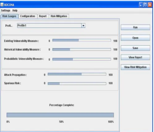
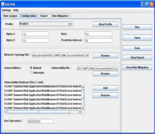
To simplify the network risk measurement and mitigation using our proposed framework, we have implemented the measures in a tool called Risk based prOactive seCurity cOnfiguration maNAger (ROCONA). We have used Java Programming Language for this implementation. The tool can run as a daemon process and therefore provide system administrators with periodic risk updates. It provides risk scores for each of the 5 components. The measures are provided as risk gauges. The risk is shown as a value between 0 and 100 as can be seen from Fig.2. The users can setup different profiles for each run of the risk measurement. They can also configure different options like parameters forEVM,AHVMandPVMand the topology and vulnerability database files to consider during vulnerability measurement. Such parameters include:
1. Thea1anda2weights required for measurement ofEVM. 2. The decay factorb in the measurement ofAHVM.
3. ThePrediction Intervalparameter(T)inPVMmeasurement.
4. The network topology file describing the interconnections between the nodes within the network.
5. The .xml files containing the list of vulnerabilities from theNVD.
6. Options for manually providing the list ofCVE vulnerabilities present in the system or to automatically extract them from third party vulnerability scanning software. The current version can only useNessusfor the automatic option. 7. The starting date from which vulnerabilities are considered (for example, all
vulnerabilities from 01/01/2004)
All these configuration options are shown in Fig.3. After the tool completes its run, it provides the system administrator with the measurement process in details. All the details can be seen in theDetails tab. Using all the gauges,ROCONAalso provides risk mitigation strategies, (i.e., which service needs to patched, how rigorous firewall policies should be) in theRisk Mitigationtab. All this information can be saved for future reference or for comparison purposes.
3.1 Deployment and Case Study
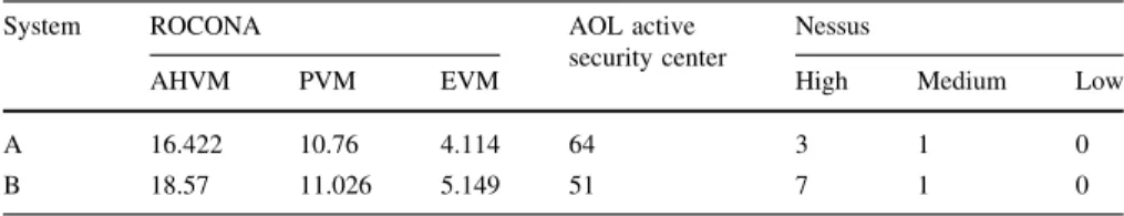
TheROCONAtool has both server and client sides. The client side is installed on individual computers in the system whereas the server part is installed for the administrator of the system. Each client communicates with the server to get the parameter values provided by the administrator. Third party softwares must also be installed so that the client program can extract the services currently running on a particular computer. The client side then sends the scores for individual components to the server where all the scores are combined to provide a unified score for the whole network system. We deployed our tool in two of our computer systems inThe University of Texas at Dallas Database and Data Mining Laboratoryto perform a comparative analysis of the risk for both the machines. Since both the machines are in the same network and under the same firewall rules, theAPandSPRvalues have been ignored (i.e., they are equal). The comparison, therefore, includes AHVM,
PVM and EVM. The results generated by ROCONA are then compared with the results of two well known security tools AOL Active Security Monitor [8] and
Nessus. AOL Active Security Monitor (ASM) provides a score based on seven factors, which include factors like firewall, virus protection, spyware protection and p2p software.Nessuson the other hand, scans for open ports and how those ports can be used to compromise the system. Based on this, Nessus provides a report warning the user of the potential threats. In Table1, the comparison is provided.
As can be seen from the table, SystemBis more vulnerable than SystemA. For SystemB, all ofAHVM,PVMandEVMscores show higher values indicating higher security risk. The same trend can be seen using the other two tools as well. For
Table 1 ROCONA Deployment and evaluation
System ROCONA AOL active
security center
Nessus
AHVM PVM EVM High Medium Low
A 16.422 10.76 4.114 64 3 1 0
Active Security Monitor, higher value indicates lower risk and for Nessus, the numbers indicate how many high, medium or low vulnerabilities are in the system. We also performed comparisons between systems where both had the same service and softwares, but one was updated and other was not. In that case only theEVM
scores were found to be different (the updated system had lower EVM) and the
AHVMandPVMscores remained the same.
It may not be feasible to provide side-by-side comparison betweenROCONAand other tools because ROCONA offers unique features in analyzing risk such as measuring the vulnerability history trend and prediction. However, this experiment shows thatROCONAanalysis is consistent with the results of the other vulnerability analysis tools such asAOL Active Security MonitorandNessus. Another important feature of ROCONA is its dynamic nature. Since, new vulnerabilities are found frequently, for the same state (i.e., same services and network configuration) of a system, vulnerability scores will be different at two different times (if the two times are significantly apart) as new vulnerabilities may appear for the services in the system. But in such a case, bothNessus and AOL Active Security Monitorwould provide the same scores, as their criteria of security measurement would remain unchanged. So far our knowledge, there is no existing tool that can perform such dynamic risk measurement and therefore, we suffice by providing comparison with these two tools. Here the scores themselves may not provide much information about the risk but can provide a comparison over time regarding the state of security of the system. This allows effective monitoring of the risk towards the system.
4 Quality of Protection Metric (QoPM)
Although the main goal of this research is to devise new factors in measuring network security, we show here that these factors can be used as a vector or scalar elements for evaluating or comparing system security or risk. For a systemS, we can combine EVM(S), AHVM(S), PVM(S), AP(S) and SPR(S) into one Total Vulner-ability Measure,TVM(S), as a vector containing all these 5 measures as in (18).
TVMðSÞ ¼½EVMðSÞ AHVMðSÞ PVMðSÞ APðSÞ SPRðSÞT ð18Þ We define theQuality of Protection Metric of systemS,QoPM(S), as in (19).
QoPMðSÞ ¼10ec1EVMðSÞ ec2AHVMðSÞ ec3PVMðSÞ ec4ð10APðSÞÞ ec5SPRðSÞT ð19Þ This will assign the value of½10 10 10 10 10Tto a system withTVMof½0 0 0 0 0T. The component values assigned by this equation will be monotonically decreasing functions of the components of theTotal Vulnerability Measureof the system. The parametersc1,c2,c3,c4andc5provide control over how fast the components of the
Quality of Protection Metric (QoPM)decreases with the risk factors. The QoPM
can be converted from a vector value to a scalar value by a suitable transformation, like taking the norm or using weighted averaging. In order to compare two systems,
we can perform the comparison of their correspondingQoPMvectors component-wise or we can convert them to scalar values and then compare those scalars. Intuitively, one way to combine these factors is to choose the maximum risk factor as the dominating one (e.g., vulnerability risk vs. spurious risk) and then measure the impact of this risk using the policy resistance measure. Although we advocate generating a combined metric, we also believe that this combination framework should be customizable to accommodate user preferences (e.g., benefit, sensitivity or mission criticality), which, however, is beyond the scope of this paper. Another important aspect of this score is that, for the vulnerability measures (i.e., EVM,
AHVM, PVM), higher score indicates higher risk or low security, whereas for
QoPM, it is the opposite. In case ofQoPM, higher score indicates higher level of security or lower risk towards the system.
5 Experimentatal Evaluation
We conducted extensive experiments for evaluating our metric using real vulnerability data. In contrast to other similar research works that present studies on a few specific systems and products, we experimented using publicly available vulnerability databases. We evaluated and tested our metric, both component-wise and as a whole, on a large number of services and randomly generated policies. In our evaluation process, we divided the data into training sets and test sets. In the following sections, we describe our experiments and present their results.
5.1 Vulnerability Database
In our experiments, we used theNational Vulnerability Database (NVD)published by National Institute of Science and Technology (NIST) which is available at
http://nvd.nist.gov/download.cfm. The NVD provides a rich array of information that makes it the vulnerability database of choice. First of all, all the vulnerabilities are stored using the standard CVE (Common Vulnerabilities and Exposures) name
http://cve.mitre.org/. For each vulnerability, the NVD provides the products and versions affected, descriptions, impacts, cross-references, solutions, loss types, vul-nerability types, the severity class and score, etc. TheNVDseverity score has a range of (0, 10). If severity value is from 0 to 4, it is considered as low severity, scores up to 7 is
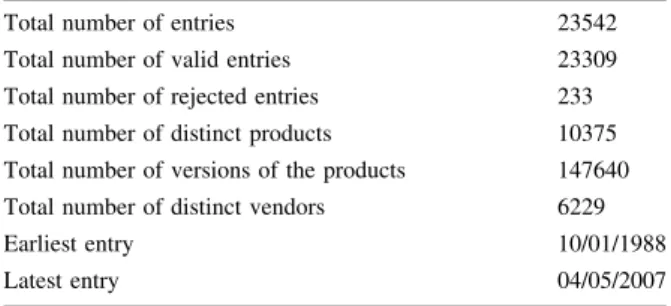
Table 2 Summary statistics of
the NVD vulnerability database Total number of entries 23542
Total number of valid entries 23309
Total number of rejected entries 233
Total number of distinct products 10375
Total number of versions of the products 147640
Total number of distinct vendors 6229
Earliest entry 10/01/1988
considered medium severity and a value higher than 7 indicates high severity. We have used the database snapshot updated at 04/05/2007. We present some summary sta-tistics about theNVDdatabase snapshot that we used in our experiments in Table 2. For each vulnerability in the database, NVD provides CVSS scores [9] for vulnerabilities in the range 1 to 10. The severity score is calculated using the
Common Vulnerability Scoring System (CVSS), which provides a base score depending on several factors like impact, access complexity, required authentication level, etc.
5.2 HVM Validation
We conducted an experiment to evaluate theHVMscore according to (1), with the hypothesis that if serviceAhas a higherHVMthan serviceB, then in the next period of time, serviceAwill display a higher number of vulnerabilities thanB.
In our experiment, we used vulnerability data upto 06/30/2006 to compute the
HVMof the services, and used the rest of the data to validate the result. We variedb
so that the decay function falls to 0.1 in 0.5, 1 , 1.5 and 2 years respectively, and observed the best accuracy in the first case. Here, we first chose services with at least 10 vulnerabilities in their lifetimes, and gradually increased this lower limit and observed that the accuracy increases with the lower limit. As expected of a historical measure, better results have been found when more history is available for the services and observed the maximum accuracy of 83.33%. The graph in Fig.4a presents the results of this experiment.
5.3 Expected Risk (ER) Validation
The experiment for the validation ofExpected Risk (ER), is divided into a number of parts. First, we conducted experiments to evaluate the different ways of calculating the probability in (3). We conducted experiments to compare the accuracies obtained by the exponential distribution, empirical distribution and time series analysis method. Our general approach was to partition the data into training and
20 40 60 80 100 0 40 80 120 160 200 Accuracy (%)
Minimum Number of Vulnerabilities per Service
HVM Accuracy β = 0.0128 β = 0.0064 β = 0.0043 β = 0.0032 40 50 60 70 80 90 100 0 10 20 30 40 50 Accuracy (%)
Training Data Set Size (Months)
Accuracy of Expected Severity
Test Size = 6 Test Size = 9 Test Size = 12
(a) (b)
Fig. 4 (a) Accuracy of the HVM for different values ofband minimum number of vulnerabilities.
(b) Training data set size versus accuracy graph for the expected severity calculation for different values of the test data set size
test data sets, compute the quantities of interest from the training data sets and validate the computed quantity using the test data sets. Here, we obtained the most accurate and stable results usingExponential CDF.
The data used in the experiment forExponential CDFwas the interarrival times for the vulnerability exposures for the services in the database. We varied the length of the training data and the test data set. We only considered those services that have at least 10 distinct vulnerability release dates in the 48 months training period. For
Expected Severity, we used similar approach. For evaluatingExpected Risk (ER), we combined the data sets for the probability calculation methods and the data sets of the expected severity.
In the experiment for Exponential CDF, we constructed an exponential distribution for the interarrival time data and computed (3) using the formula in (7). For each training set, we varied the value ofT, and ran validation for each value of T with the test data set. Fig.5a presents the accuracy of the computed probabilities usingExponential CDFmethod for different training data set sizes and different values of the Prediction Interval parameter, T. In Fig.5b, we have
0 30 60 90 120 20 30 40 50 60 Accuracy (%)
Training Data Set Size (Months) Accuracy of Exponential CDF Method
T = 15 T = 30 T = 45 T = 60 T = 75 T = 90 0 20 40 60 80 0 20 40 60 80 100 Accuracy (%)
Prediction Interval, T (Days) Accuracy of Exponential CDF Method
Train Size = 24 Train Size = 30 Train Size = 36 Train Size = 42 Train Size = 48 (a) (b)
Fig. 5 (a) Training data set size versus accuracy graph for the exponential CDF method for probability
calculation, test set size = 12 months. (b) Prediction interval parameter (T) versus accuracy graph for the exponential CDF method for probability calculation, test set size = 12 months
30 45 60 75 20 25 30 35 40 45 50 Accuracy (%)
Train Data Set Size (Months) Expected Risk Accuracy
Test Size = 6 Test Size = 9 Test Size = 12 15 30 45 60 75 6 9 12 Accuracy (%)
Test Data Set Size (Months) Expected Risk Accuracy
Train Size = 24 Train Size = 30 Train Size = 36 Train Size = 42 Train Size = 48 (a) (b)
Fig. 6 (a) Results of ER validation with training data set size versus accuracy for different test data set sizes.
presented the accuracies on theYaxis against thePrediction IntervalparameterTon theXaxis. For the test data set size of 12 months, we observed the highest accuracy of 78.62% with the 95% confidence interval being 72½ :37;84:87 for the training data set size of 42 months andPrediction Intervalof 90 days. We present the results of the experiment for Expected Severity in Fig.4b. The maximum accuracy obtained in this experiment was 98.94% for the training data set size of 3 months and the test data set size of 9 months. The results of theExpected Riskexperiment are presented in the Fig.6a and b. For the Expected Risk, we observed the best accuracy of 70.77% for training data set size of 24 months and test data set size of 12 months with the 95% confidence interval of 64½ :40;77:14.
It can be observed in Fig.5b that the accuracy of the model increases with increasing values of the Prediction Interval parameter T. This implies that this method is not sensitive to the volume of training data available to it. From Fig.4b, it is readily observable that the accuracy of theExpected Severityis not dependent on the test data set size. It increases quite sharply with decreasing values of training data set data size. This means that the expectation calculated from the most recent data is actually the best model for the expected severity in the test data.
5.4 QoPM Validation
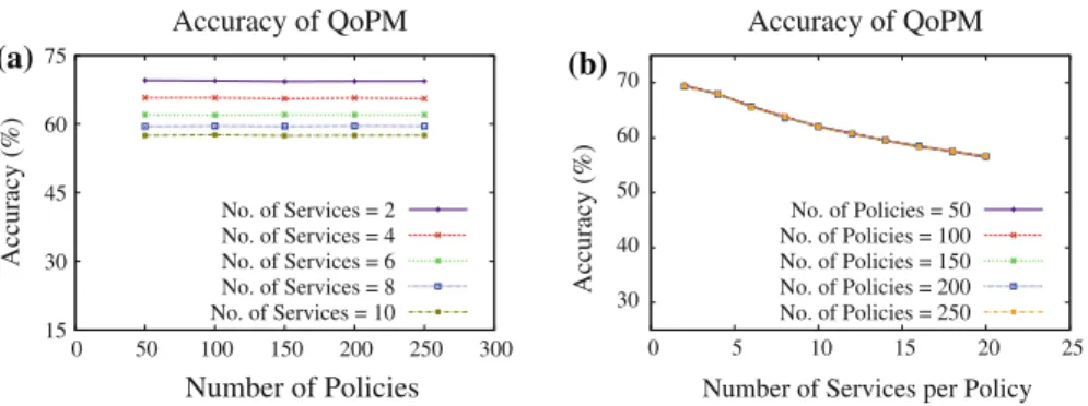
To validate theQoPM, we need to evaluate policies using our proposed metric in (19). In absence of other comparable measures of system security, we used the following hypothesis – if system A has a better QoPM than system B based on training period data, then system A will have less number of vulnerabilities than systemBin the test period. We assume that theEVMcomponent of the measure will be 0 as any existing vulnerability can be removed.
In generating the data set, we chose the reference date separating the training and test periods to be 10/16/2005. We used the training data set forERusingExponential CDFmethod. In the experiment, we generated a set of random policies and for each policy we evaluated (19). We chosec1=c2=c3=c4=c5=0.06931472 so that the QoPMfor a TVM of ½10 10 10 10 10T is ½5 5 5 5 5T. Then, for each pair of
15 30 45 60 75 0 50 100 150 200 250 300 Accuracy (%) Number of Policies Accuracy of QoPM No. of Services = 2 No. of Services = 4 No. of Services = 6 No. of Services = 8 No. of Services = 10 30 40 50 60 70 0 5 10 15 20 25 Accuracy (%)
Number of Services per Policy
Accuracy of QoPM No. of Policies = 50 No. of Policies = 100 No. of Policies = 150 No. of Policies = 200 No. of Policies = 250 (a) (b)
Fig. 7 (a) Number of policies versus accuracy graph for QoPM for different values of the number of
services in each policy. (b) Number of services per policy versus accuracy graph for QoPM for different values of the number of policies
systemsAandB, we evaluated the hypothesis that ifQoPM(A)C QoPM(B) then, the number of vulnerabilities for serviceAshould be less than or equal to the number of vulnerabilities for serviceB. In our experiment, we varied the number of policies from 50 to 250 in steps of 25. In generating the policies, we varied the number of services per system from 2 to 20 in increments of 2.
We present the results obtained by the experiment in Fig.7a and b. As mentioned previously, a policy can be regarded as a set of rules indicating which services are allowed access to the network traffic. We set up different service combinations and consider them as separate policies for our experiments. We can observe from the graph in Fig.7a that the accuracy of the model is not at all sensitive to the variation in the total number of policies. However, the accuracy does vary with the number of services per policy – the accuracy decreases with increasing number of services per policy. This trend is more clearly illustrated in Fig.7b where the negative correlation is clearly visible.
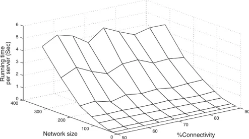
5.5 Running Time Evaluation of Attack Propagation Metric
To assess the feasibility of calculating theAPmetric under different conditions, we ran aMatLabimplementation of the algorithm for different network sizes, as well as different levels of network connectivity percentages (the average percentage of the network directly reachable from a host). The machine used to run the simulation had a 1.9 GHz P-IV processor with 768MB RAM. The results are shown in Fig.8. For each network size, we generated several random networks with the same %connectivity value. The running time was then calculated for several hosts within each network. The average value of the running time per host was then calculated and used in Fig.8. As can be seen from the figure, the quadratic growth of the running time against network connectivity was not noticeably dependent on the
50 60 70 80 90 0 100 200 300 400 0 1 2 3 4 5 6 %Connectivity Network size
Running time per server (Sec)
network %connectivity in our implementation. The highest running time per host for a network of 320 nodes was very reasonable at less than 5 seconds. Thus, the algorithm scales gracefully in practice and is thus feasible to run for a wide range of network sizes.
6 Related Work
Measurement of network and system security has always been an important aspect of research. Keeping this in mind, many organizational standards have been evolved to evaluate the security of an organization. National Security Agency’s (NSA) INFOSEC Evaluation Methodology (IEM) can be mentioned as an example in this respect. Details regarding the methodology can be found in [10]. In [11] NIST provides a guidance to measure and strengthen the security through the development and use of metrics, but their guideline is focused on the individual organizations and they do not provide any general scheme for quality evaluation of a policy. There are some professional organizations as well as vulnerability assessment tools including Nessus, NRAT, Retina, Bastille and others [12]. They actually try to find out vulnerabilities from the configuration information of the concerned network. However, all these approaches usually provide a report telling what should be done to keep the organization secure and they do not consider the vulnerability history of the deployed services or policy structure.
There has been a lot of research in the security policy evaluation and verification as well. Evaluation of VPN, Firewall and Firewall security policies include [6,7,
13]. Attack graphs is another technique that is well developed to assess the risks associated with network exploits. The implementations normally require intimate knowledge of the steps of attacks to be analyzed for every host in the network [14,
15]. In [16] the authors, however, provide a way to do so even when the information is not complete. Still, this setup causes the modeling and analysis using this model to be highly complex and costly. Mehta et al. try to rank the states of an attack graph in [17]. But their work do not give any sort of prediction of future risks associated with the system and also, they do not consider the policy resistance of firewall and IDS. Our technique that is employed to assess the policy’s immunity to attack propagation implements a simpler and less computationally expensive technique that is more suitable for our goal.
There has been some research focusing on the attack surface of a network. Mandhata et al. in [18] have tried to find the attack surface from the attackability of a system. Another work based on attack surface has been done by Howard et al. in [19] along channel, methods and data dimensions and the contributions of these dimensions in an attack. A. Atzeni et al. present a generic overall framework for network security evaluation in [20], and discuss the importance of security metrics in [21]. In [22] Pamula propose a security metric based on the weakest adversary (i.e. the least amount of effort required to make an attack successful). In Alhazmi et al. [1], present their results on the prediction of vulnerabilities and they present their work on vulnerability discovery process in [23]. They argue that vulnerabilities are essentially defects in released software and uses past data and track records of
the development team, code size, records of similar softwares etc. to predict the number of vulnerabilities. Our work is more general in this respect and utilizes publicly available data.
There has also been some research work that focus on hardening the network. Wang et al. use attack graphs for this purpose in [24]. They also attempt to predict future alerts in multistep attacks using attack graph [25]. A previous work of hardening the network was done by Noel et al. [26] where they made use of dependencies among exploits. They use the graphs to find some initial conditions that, when disabled, will achieve the purpose of hardening the network. Sahinoglu et al. propose a framework in [27, 28] for calculating existing risk depending on present vulnerabilities in terms of threat represented as probability of exploiting this vulnerability and the lack of counter-measures. But all these work do not represent the total picture as they predominantly try to find existing risk and do not address how risky the system will be in the near future or how policy structure would impact on security. Their analysis regarding security policies can not be regarded as complete and they lack the flexibility in evaluating them.
A preliminary investigation of measuring the existing vulnerability and some historical trends have been analyzed in a previous work [29]. That work was still limited in analysis and scope.
7 Conclusions
As network security is of utmost importance for an organization, a unified policy evaluation metric will be highly effective in assessing the protection of the current policy, and justifying consequent decisions to strengthen security. In this paper, we present a proactive approach to quantitatively evaluate security of network systems by identifying, formulating and validating several important factors that greatly affect its security. Our experiments validate our hypothesis that if a service has a highly vulnerability prone history, then there is higher probability that the service will become vulnerable again in the near future. These metrics also indicate how the internal firewall policies affect the security of the network as a whole. These metrics are useful not only for administrators to evaluate policy/network changes and, take timely and judicious decisions, but also for enablingadaptive security systemsbased on vulnerability and network changes.
Our experiments provide very promising results regarding our metric. Our vulnerability prediction model proved to be up to 78% accurate, while the accuracy level of our historical vulnerability measurement was 83.33% based on real-life data from National Vulnerability Database (NVD). The accuracies obtained in these experiments vindicate our claims about the components of our metric and also the metric as a whole. Combining all the measures into a single metric and performing experiments based on this single metric also provides us with an idea of its effectiveness.
Acknowledgments The authors would like to thank Muhammad Abedin and Syeda Nessa of The
University of Texas at Dallas for their help with the formalization and experiments making this work possible.
References
1. Alhazmi, O.H., Malaiya Y.K.: Prediction capabilities of vulnerability discovery models. In: Pro-ceedings of reliability and maintainability symposium, Jan 2006, pp. 86–91
2. National institute of science and technology (nist),http://nvd.nist.gov
3. Lee, S.C., Davis, L.B.: Learning from experience: operating system vulnerability trends, IT Pro-fessional,5(1), Jan/Feb 2003
4. Abedin, M., Nessa, S., Al-Shaer, E., Khan, L.: Vulnerability analysis for evaluating quality of protection of security policies, In: 2nd ACM CCS workshop on quality of protection, Alexandria, Virginia, Oct 2006
5. Bock, F.: An algorithm to construct a minimum directed spanning tree in a directed network, In: Developments in Operations Research. Gordon and Breach, pp. 29–44 (1971)
6. Al-Shaer, E., Hamed, H.: Discovery of policy anomalies in distributed firewalls. In: Proceedings of IEEE INFOCOM’04, March 2004
7. Hamed, H., Al-Shaer, E., Marrero, W.: Modeling and verification of ipsec and vpn security policies. In Proceedings of IEEE ICNP’2005, Nov 2005
8. Aol software to improve pc security, http://www.timewarner.com/corp/newsroom/pr/0,20812, 1201969,00.html
9. Schiffman, M.: A complete guide to the common vulnerability scoring system (cvss). http://www.first.org/cvss/cvss-guide.html, June 2005
10. Rogers, R., Fuller, E., Miles, G., Hoagberg, M., Schack, T. Dykstra, T., Cunningham, B.: Network Security Evaluation Using the NSA IEM, 1st ed. Syngress Publishing, Inc., Aug 2005
11. Swanson, M., Bartol, N., Sabato, J., Hash, J., Graffo, L.: Security Metrics Guide for Information Technology Systems. National Institute of Standards and Technology, Gaithersburg, MD 20899-8933, July 2003
12. ’’10 network security assessment tools you can’t live without’’ http://www.windowsitpro.com/ Article/ArticleID/47648/47648.html?Ad=1
13. Kamara, S., Fahmy, S., Schultz, E., Kerschbaum, F., Frantzen, M.: Analysis of vulnerabilities in internet firewalls. Comput. Secur.22(3), 214–232 (2003)
14. Ammann, P., Wijesekera, D., Kaushik, S.: Scalable, graph-based network vulnerability analysis. In: CCS ’02: Proceedings of the 9th ACM conference on computer and communications security, pp. 217–224, ACM Press, New York, NY, USA (2002)
15. Phillips, C., Swiler, L.P.: A graph-based system for network-vulnerability analysis. In: NSPW ’98: Proceedings of the 1998 workshop on new security paradigms, pp. 71–79, ACM Press, New York, NY, USA (1998)
16. Feng, C., Jin-Shu, S.: A flexible approach to measuring network security using attack graphs. In: International symposium on electronic commerce and security, April 2008
17. Mehta, C.B.V., Zhu, H., Clarke, E., Wing, J.: Ranking attack graphs. In: Recent Advances in Intrusion Detection 2006, Hamburg, Germany, Sept 2006
18. Manadhata, P. Wing, J.: An attack surface metric. In: First Workshop on Security Metrics, Van-couver, BC, August 2006
19. Howard, M., Pincus, J., Wing, J.M.: Measuring relative attack surfaces. In: Workshop on Advanced Developments in Software and Systems Security, Taipei, Dec 2003
20. Atzeni, A., Lioy, A., Tamburino, L.: A generic overall framework for network security evaluation. In: Congresso Annuale AICA 2005, Oct 2005, pp. 605–615
21. Atzeni, A., Lioy, A.: Why to adopt a security metric? A little survey. In: QoP-2005: Quality of protection workshop. Sept 2005
22. Pamula, J., Ammann, P., Jajodia, S., Swarup, V.: A weakest-adversary security metric for network configuration security analysis. In: ACM 2nd workshop on quality of protection 2006, Alexandria, VA, Oct 2006
23. Alhazmi, O.H., Malaiya, Y.K.: Modeling the vulnerability discovery process. In: Proceedings of international symposium on software reliability engineering, Nov 2005
24. Wang, L., Noel, S., Jajodia, S.: Minimum-cost network hardening using attack graphs. In: Computer Communications. Alexandria, VA, Nov 2006
25. Wang, L., Liu, A., Jajodia, S.: Using attack graphs for correlating, hypothesizing, and predicting intrusion alerts. In: Computer Communications, Sept 2006
26. Noel, S., Jajodia, S., O’Berry, B., Jacobs, M.: Efficient minimum-cost network hardening via exploit dependency graphs. In: 19th annual computer security applications conference, Las Vegas, Nevada, Dec 2003
27. Sahinoglu, M.: Security meter: a practical decision-tree model to quantify risk. In: IEEE Security and Privacy, June 2005
28. Sahinoglu, M.: Quantitative risk assessment for dependent vulnerabilities. In: Reliability and maintainability symposium, June 2005
29. Ahmed, M.S., Al-Shaer, E., Khan, L.: A novel quantitative approach for measuring network security. In: INFOCOM’08, April 2008
Author Biographies
Mohammad Salim Ahmedis currently working toward his Ph.D. degree in the Department of Computer
Science at the University of Texas at Dallas (UTD). He graduated from Bangladesh University of Engineering and Technology with BS in Computer Science and Engineering degree in 2005. He was also a Lecturer of the same university. His research interests are in text mining, machine learning, and network security measurement using data mining. His recent research focuses on developing data mining techniques to classify high dimensional text data. He has published more than 5 research papers in peer reviewed conferences and workshops including INFOCOM, NOMS, DDDM and CIDU.
Ehab Al-Shaer is an Associate Professor and the Director of the Cyber Defense and Network
Assurability (CyberDNA) Center in the School of Computing and Informatics at University of North Carolina Charlotte. His primary research areas are network security, security management, fault diagnosis, and network assurability. Al-Shaer edited/co-edited more than 10 books and book chapters, and published many refereed journals and conference papers in his area. Prof. Al-Shaer is the General Chair of ACM Computer and Communication 2009-2010 and NSF Workshop in Assurable and Usable Security Configuration, August 2008. Prof. Al-Shaer also served as a Workshop Chair and Program Co-chair for number of well-established conferences/workshops in his area including POLICY 2008, IM 2007, ANM-INFOCOM 2008, CCS-SafeConfig 09, MMNS 2001, and E2EMON 04-05. He also served as a member in the technical program and organization committees for many IEEE and ACM conferences. He was awarded many Best Paper Awards. Prof. Al-Shaer received his MSc and Ph.D. in Computer Science from the Northeastern University (Boston, MA) and Old Dominion University (Norfolk, VA) in 1998 and 1994 respectively.
Mohamed Taibahis a PhD student at DePaul University. He had his BSc and MS degrees in Electrical
Engineering from King Fahd University of Petroleum and Minerals, Saudi Arabia and Northwestern University, Chicago, USA in 1996 and 1999 respectively. His area of research is worm control, botnet detection and risk measurement. He is currently working with Cisco
Latifur Khanis currently an Associate Professor in the Computer Science department at the University
of Texas at Dallas (UTD), where he has taught and conducted research since September 2000. He received his Ph.D. and M.S. degrees in Computer Science from the University of Southern California, in August of 2000, and December of 1996 respectively. His research work is supported by grants from NASA, the Air Force Office of Scientific Research (AFOSR), National Science Foundation (NSF), IARPA, the Nokia Research Center, Raytheon, Alcatel, and the SUN Academic Equipment Grant program. In addition, Dr. Khan is the director of the state-of-the-art DBL@UTD, UTD Data Mining/ Database Laboratory, which is the primary center of research related to data mining, and image/video annotation at University of Texas-Dallas. Dr. Khan’s research areas cover data mining, multimedia information management, semantic web and database systems with the primary focus on first three research disciplines. He has served as a committee member in numerous prestigious conferences, symposiums and workshops including the ACM SIGKDD Conference on Knowledge Discovery and Data Mining. Dr. Khan has published over 130 papers in journals and conferences.