An Efficient Multi-Dimensional Index for Cloud Data Management

(1)

An Efficient Multi-Dimensional Index for Cloud Data

Management

Xiangyu Zhang, Jing Ai, Zhongyuan Wang, Jiaheng Lu, Xiaofeng Meng

School of Information, Renmin University of China

Beijing, China, 100872

[email protected] {aijingruc,zhywang,xfmeng}@ruc.edu.cn [email protected]

ABSTRACT

Recently, the cloud computing platform is getting more and more attentions as a new trend of data management. Currently there are several cloud computing products that can provide various ser-vices. However, currently the cloud platforms only support sim-ple keyword-based queries and can’t answer comsim-plex queries effi-ciently due to lack of efficient index techniques. In this paper we propose an efficient approach to build multi-dimensional index for Cloud computing system. We use the combination of R-tree and KD-tree to organize data records and offer fast query processing and efficient index maintenance. Our approach can process typ-ical multi-dimensional queries including point queries and range queries efficiently. Besides, frequent change of data on big amount of machines makes the index maintenance a challenging problem, and to cope with this problem we proposed a cost estimation-based index update strategy that can effectively update the index struc-ture. Our experiments show that our indexing techniques improve query efficiency by an order of magnitude compared with alter-native approaches, and scale well with the size of the data. Our approach is quite general and independent from the underlying in-frastructure and can be easily carried over for implementation on various Cloud computing platforms.

Categories and Subject Descriptors

C.2.4 [Computer-Communication Networks]: Distributed Sys-tems—distributed applications; H.2.4 [Database Management]: Systems—concurrency, transaction processing

General Terms

Algorithms

Keywords

multi-dimensional index, distributed index, query processing

1. INTRODUCTION

Internet has been developing at an astonishing speed. Each day a huge amounts of information is put on the Internet in the form

Permission to make digital or hard copies of all or part of this work for personal or classroom use is granted without fee provided that copies are not made or distributed for profit or commercial advantage and that copies bear this notice and the full citation on the first page. To copy otherwise, to republish, to post on servers or to redistribute to lists, requires prior specific permission and/or a fee.

of digital data. Many new Internet applications emerge and most of them require to process a large scale of data efficiently. How-ever, traditional data management tools have been insufficient for this new demands. For example, database systems softwares of-ten are multi-of-tenancy, which means that online users must share the same software’s resources simultaneously. When unexpected spikes come, users may meet the situation of shortage of resources and a drop of quality of service. Therefore, scalability is a cru-cial requirement for future Web applications. Under those circum-stances, a new computing infrastructure,cloud computing, emerges. Though the unified definition of cloud computing has not been con-firmed[1], it is considered as a revolution in IT industry. Systems supporting cloud computing dynamically allocate computational resources according to users’ requests. Existing Cloud comput-ing systems include Amazon’s Elastic Computcomput-ing Cloud(EC2)[2], IBM’s Blue Cloud[3] and Google’s MapReduce[4]. They adopt flexible resources management mechanism and provide good scal-ability. Scalable data structures can satisfy resource demands of Cloud systems’ users. Cloud computing systems are usually com-prised of a large number of computers, store huge amounts of data, and provide services for millions of users. Resources allocation is typically elastic in cloud systems, which makes each user feel that he owns infinite amount of resources. A typical example of scalable data structure is Google’s BigTable[5].

Currently, most of Cloud infrastructures are based on Distributed File Systems. DFS usually use key-value storage models to store data. The data in Cloud systems are organized in the form of key-value pairs. Therefore, current Cloud systems can only support keyword search. When a query comes, result data are retrieved from DFS in accordance with contained keywords. Although many famous Cloud systems uses this information storage pattern, such as Google’s GFS[6] and Hadoop’s HDFS[7], they only provide ser-vices of keyword queries for users. Therefore, users can only ac-cess information through "point query" which matches records to satisfy the verbal and/or numerical values.

The emergence of cloud computing is due to the need of increas-ing advanced data management. And it needs to serve a large va-riety of applications better for more Web users. Therefore, future cloud infrastructures should be developed to support more types of queries with more functions, e.g. muti-dimensional queries.

Cloud computing platforms contain hundreds and thousands of machine nodes, and they process workloads and tasks in parallel. This is a typical characteristic of cloud computing infrastructures. When a user submits a query, result data are retrieved from un-derlying storage tables and then distributed to a set of processing nodes for parallel scanning. Without the support of efficient index structure, query processing is quite time-consuming, especially for complex queries. Therefore, building more efficient index structure

(2)

is a pressing demand. Moreover, because of huge amounts of data in cloud systems, the index should be able to provide high retrieval rate.

Up to now, there are some proposals of building efficient index for cloud infrastructures. Aguilera et al.[8] proposed a scalable dis-tributed B-tree for their Cloud system. Other research work pro-posed a kind of index based on hash index structure. However, these indices just can index single column. They can not efficiently support range queries referring to multi-columns’ data.

In order to support range queries efficiently in the Cloud system, we present a scalable and flexible multi-dimensional index struc-ture based on the combination of R-Tree and KD-tree.

In summary, this paper makes the following contributions:

• We propose an efficient and scalable multi-dimensional in-dex structure. With this structure we can answer typical point queries and range queries efficiently. Our index scales very well as the data volume or cluster size grows.

• We propose a cost estimation-based index update strategy. With this strategy we can assure that update will only be done when it’s necessary and the benefit of update is ensured.

• We perform a series of experiments on large scale of machine nodes with large volume of data. The experiment confirms that our index structure is quite efficient and scalable.

2. RELATED WORK

Cloud computing brings new ways of Web services for Web users and enterprises. There have been some cloud computing systems. Typical examples include Amazon’s Elastic Computing Cloud(EC2)[2], and IBM’s Blue Cloud[3] and Google’s MapRe-duce[4]. These systems designed for cloud computing usually only support basic key/value based queries, and lacks more efficient in-dex structures.

The concept of cloud computing initially comes from search en-gines’ infrastructure. Unlike DBMS, search engines usually does not adopt order-preserving tree indexes, such as B-tree or hash ta-ble. To improve performance and support more types of queries, some works tried to build index on cloud computing platforms. The work in [9] proposed an extension of MapReduce to join het-erogeneous datasets and execute relational algebra operations. And searching tree indexes were built in bulk MapReduce operations. However, this work mainly focused on improving search engines’ performances and might lack generality when used in cloud com-puting platforms.

B-tree is a very commonly used index in database management systems, and most prior work on B-tree usually focused on ones stored in a single computer’s memory space. The work in [8] pre-sented a more general and flexible index structure: a fault-tolerant and scalable distributed B-tree for cloud systems. Distributed trans-actions is used to make changes to B-tree nodes. B-tree nodes can be migrated online between servers for load-balancing. This design is based on a distributed data sharing service, Sinfonia[10], which provides fault tolerance and a light-weight distributed atomic prim-itive. However, this index schema may cause high memory over-head because of inner nodes’ replication, especially for client com-puters. Moreover, although B-tree has been widely used as single-attribute index in database systems, it is inefficient in dealing with indices composed of multi-attributes.

The paper by S. Wu and K.-L. Wu[11] proposed an improved indexing framework for cloud systems. This indexing framework supports all existing index structures. The hash index and B+_-tree

index are used to demonstrate the effectiveness of the framework.

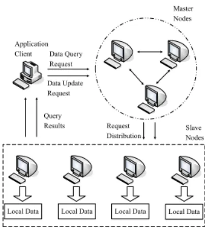
Figure 1: Framework of Request Processing in Cloud

And machine nodes are organized in a structured Peer-to-Peer net-work which can effectively reduce the index maintenance cost. Al-though this index schema is scalable and flexible, the Peer-to-Peer structure is not very suitable for cloud systems.

There are also some algorithms of distributed B-tree in distributed file systems and databases(e.g.,[12, 13]). However, these distributed B-tree indices can not support multi-dimensional query answering effectively. Because even if an attribute column in the data table is indexed by a distributed B-tree, answering multi-dimensional queries still need to find eligible result records on other attributes. And query answering is still possible to have long response time.

Much work on distributed index structures has been done by re-searchers, such as distributed hash tables(DHT) (e.g. [14, 15]). However, these indexes in [14, 15, 16] are designed and deployed on Peer-to-Peer data structures. Although some DHT extensions can support range queries[16], P2P structures work with little syn-chrony and may cause weak even no consistency. In contrast, cloud systems must be able to provide certain level of consistency. More-over, nodes in P2P structures are equal with each other. Cloud sys-tem has master nodes which are responsible for distributing com-puting tasks and resources to slave nodes. Therefore, these dis-tributed hash index can’t meet the demand of cloud systems.

In contrast with that, our distributed index can efficiently support various queries(e.g. point query, range query), and provide high retrieve and update rates.

3. QUERYING AND UPDATE IN THE CLOUD

As a basic characteristic of the cloud platform, a cluster consist-ing of hundreds or thousands of PC is responsible for the mission of computing and storage of data. As Figure 1 shows, machine nodes in the cluster can be categorized into two types: master nodes and slave nodes. Master nodes and slave nodes are not too much dif-ferent except that if a machine is playing the role of master node it will store some meta data about the whole system along with other regular data that slave nodes also have to store. Slave nodes store data records and their replicas for efficiency and security. Al-though one of the distinguishing characteristics of Cloud platform from the Client-Server architecture based systems is that the Cloud systems don’t need central servers, it still needs a set of machines to maintain meta data about the whole system, and this makes many operations more efficient.

In the cloud platform, client requests are often posed against the master nodes. After that the master nodes decide which slave nodes are relevant to the request and then the client will communicate

(3)

with those nodes directly. The framework of request process in cloud platform is in Figure 1. So as a typical request, query pro-cessing in the cloud platform can be divided into two phases: lo-cating relative nodes and processing the request on selected slave nodes. The procedure could be expressed as algorithm 1.

Algorithm 1Process query on cloud

1: procedureSET PROCESSQUERY(Query q) 2: Set nodes = empty;

3: nodes.add(getRelativeNodes(q)); 4: Set results = empty;

5: for(each nodenin thenodes)do

6: results.add(n.retrieveRecords(q)); 7: end for

8: returnresults; 9: end procedure

Maintenance of the index upon data insertion and deletion is also a major aspect of an index. Like the query processing procedure, insertion and deletion can also be divided into locating relative nodes and performing the operation on relative nodes. The two procedures can be described as algorithm 2 and 3:

Algorithm 2Record insertion to cloud

1: procedureBOOLEAN INSERTRECORD(Record r) 2: Set nodeSet = empty;

3: nodeSet.add(getNodesForRecord(r)); 4: for(each nodeninnodeS et)do

5: if(n.insertRecord(r) == false)then

6: returnfalse; 7: end if

8: end for

9: returntrue; 10: end procedure

Algorithm 3Record deletion from cloud 1: procedureINT DELETERECORDS(Query q) 2: Set nodeSet = empty;

3: nodeSet.add(getRelativeNodes(q)); 4: int count = 0;

5: for(each nodenin thenodeS et)do

6: count += n.deleteRecords(q); 7: end for

8: returncount; 9: end procedure

From the above discussion we can see that the key functional components of a multi-dimensional index are:

Query Processing

• Locating relative slave nodes for query

• Processing query on each slave node and fetch results

Index Maintenance

• Locating appropriate slave nodes for record insertion

• Locating relative slave nodes for data deletion (same as that in query processing)

• Inserting records into individual slave node

• Deleting records from individual slave node

In the following part of the paper, we will discuss how to build and maintain multi-dimensional indices in cloud computing en-vironment by conducting the 6 key functional components listed above.

4. MULTI-DIMENSIONAL INDEX

As the Cloud computing platform can be considered as a cluster of PC machines, we can build a global index of the platform by building local indices on each individual machine. Requests to the virtual global index could be answered by executing the query on local indices and then combining the returned results. Before in-troducing our index approach, we give a short introduction to the structures we will use.

4.1 R-Tree and KD-tree

R-tree[17] is a popular multi-dimensional index, which is usually used in spatial and multi-dimensional applications. R-tree index is a data structure that captures some of the spirit of the B-tree for multi-dimensional data. A R-tree index represents data that con-sists of 2-dimensional, or higher dimensional regions. An interior node of an R-tree corresponds to some interior region. In principle, the region can be of any shape.

A kd-tree[18] is a binary tree in which each interior node has an associated attribute a and a value V that splits the data points into two parts: those with a-value less than V and those with a-value equal to or greater than V. The attributes at different levels of the tree are different, with levels rotating among the attributes of all dimensions.

4.2 Basic Structure

For the basic structure, we build the multi-dimensional index for the platform by building local KD-tree index for each slave nodes. The reason for our choice of KD-tree instead of other structures is that the KD-tree can efficiently support point query, partial match query and range query.

Query Processing

In the relative node locating phase we choose all the nodes in the cluster as candidates of the query since currently we don’t have the knowledge about data distribution on each slave node, and thus makes all nodes possible to contain records relative to the query. And in the record retrieving phase, each node utilizes the local KD-tree index to get records on that node. The procedures are describe as algorithm 4 and 5:

Algorithm 4Get candidate nodes to search for the query 1: procedureSET GETRELATIVENODES(Query q) 2: returnall the nodes of the platform; 3: end procedure

Algorithm 5Get records satisfying the query on the node 1: procedureSET RETRIVERECORDS(Query q) 2: Set recordSet = lookupKDTree(q); 3: returnrecordSet;

4: end procedure Index Maintenance

For data insertion, since in the basic structure there is not any metadata to consider so we only take load balance into consider-ation. Hence, we pick a set of nodes based on some load balance

(4)

Master Nodes

Slave Nodes

KD-Tree KD-Tree KD-Tree KD-Tree Request

Distribution

Bounding Bounding Bounding Bounding

(700,200) (500,400) (900,600) (200,300) (400,700) (800,100) (950,900) (700,200) (500,400) (900,600) (200,300) (400,700) (800,100) (950,900) (700,200) (500,400) (900,600) (200,300) (400,700) (800,100) (950,900) (700,200) (500,400) (900,600) (200,300) (400,700) (800,100) (950,900) R1R2 R3R4R5 R6R7 R8R9R10 R11R12 R13R14 R15R16 R17R18R19 R-Tree

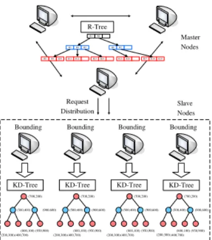
Figure 2: Framework of EMINC

approach, which is not the focus of this paper so we will not discuss it. After that, we apply the insert function defined on the local KD-tree. For data deletion, as each node is a potential node for query processing, we need to perform local deletion on every slave node.

4.3 Pruning Irrelevant Nodes with R-tree

The approach we have shown distributes local indices on slave nodes without maintaining any meta-data and this directly leads to inefficiency of query processing. The efficiency of locating relative nodes can be improved by maintaining bounding information of each dimension on each node and prune irrelevant nodes during query processing.

To prune irrelevant nodes on query processing, we construct a

node cubefor each slave node. A node cube indicates the range of

value on each indexed attribute in this node.

Definition 1. Anode cubeis a sequence of value intervals, and

each interval represents the value range of one indexed attribute on this node. If there’s only one value on some dimension, the corresponding interval regresses to a value point.

Example 1 :If we construct a two-dimension index on attributeage

andsalaryof a table, we can make a node cube of {[30, 40], [100,

200]} meaning that records on this node haveageattribute between 30 and 40 andsalaryattribute between 100 and 200.

After we build a cube for each slave node, we maintain the cubes on master nodes with an R-tree. The reason why we choose R-tree instead of KD-tree for cube information is that the R-tree was de-signed for managing data regions and in our scenario the cubes are actually multi-dimensional data regions. We call this index approach EMINC: Efficient Multi-dimensional Index with Node Cube. Framework of EMINC is shown in Figure 2

Definition 2. EMINCindex structure consists of a R-tree in

mas-ter nodes and one KD-tree on each slave node. Each leaf node of the R-tree contains a node cube and one or more pointers that point to the slave nodes corresponding to the node cube.

With the node cube information in EMINC, query processing can be greatly improved by pruning irrelative nodes in the nodes locating phase. And in order to keep cube information available and useful, insertion and deletion on slave nodes that may change their cubes should inform master nodes for update of cube.

Query Processing

When a query is posed, we first get the key value or key range on each demand, construct aquery cubefor query. Query cube is an analogy concept to node cube with the following definition:

Definition 3. Aquery cubeis a sequence of intervals, and each

interval represents the value range of one attribute in this query. If either side of the attribute is not specified, we assign it the biggest negative or positive value accordingly.

With the query cube we resort to the R-tree for nodes that are re-lated to the query by issuing the classic "where am I" query. Specif-ically, we look up the R-tree to find those slave nodes whose node cubes intersect with the query cube of the query. The definition of cube intersection is as follows:

Definition 4. Intersection of two cubes (node cube or query

cube) means that for each attribute the two corresponding inter-vals must have overlap. If one of the two interinter-vals has regressed to a point, then the intersection semantic is replaced by the inter-val containing the point or the two points being equal, depending whether there is one point or two.

We can see from the definition of intersection that this can be done with the typical "where am I" query on R-tree. And only the intersecting nodes are possible to contain records satisfying the query, so that a big part of irrelevant nodes are pruned. After locat-ing relative nodes, we do local search on the slave node. The new nodes locating procedure is as algorithm 6:

Algorithm 6Get candidate nodes using cube 1: procedureSET GETRELATIVENODES(Query q)

2: QueryCube cube = getCubeForQuery(Query q); 3: Set nodeSet = getNodesForCube(cube); 4: returnnodeSet;

5: end procedure Index Maintenance

In order for the node cube information to stay effective, we have to update the cube on master nodes if the cube is out-of-date due to data insertion or deletion on slave nodes. If the cube information on master nodes is not updated in time, the query processing will either miss relative records or search more irrelative nodes.

Recall that the first step of data insertion is to select the appro-priate slave nodes to insert to. Selection of nodes can affect future query processing efficiency. If we can select the nodes in a way that data records are "clustered" by their indexed attribute values, then future query processing can benefit greatly from this since less slave nodes need to be explored for one query. Based on this idea, we try to give such nodes higher priority in data insertion : nodes that have node cube that can cover the record to be inserted, and by cover we mean that each indexed value of the record is in the corresponding interval of the node cube. Under this principle, the node selection procedure is shown as algorithm 7.

After selecting the nodes to insert to, record is inserted into them. Insertion of a new data record may cause the node cube of this node to expand on one or more dimensions if the current cube can’t enclose the new record. And if this happens, this node must inform the master node of the change and give the new node cube to master node to keep it up to date. The update on master node is a typical update operation on R-tree.

Example 2 : Suppose the current node cube is {[30, 40], [100, 200]}. If we insert a new record (42, 210), and then the new cube

(5)

Algorithm 7Select nodes for insertion 1: procedureSET SELECTNODES(Record r)

2: candidateSet = empty; 3: int count = 0;

4: for(count < replica amount)do

5: Node node = selectNodeWithCoveringCube(r); 6: if(node is not null)then

7: candidateSet.add(node);

8: else

9: // This means there is no more such nodes.

10: break from loop;

11: end if

12: end for

13: if(count < replica amount)then

14: // Choose rest of the nodes.

15: int remaining = replica amount - count; 16: // Choose nodes based on load balance, etc. 17: Set remainingSet = chooseTheRest(remaining); 18: candidateSet.add(remainingSet);

19: end if

returncandidateSet; 20: end procedure

will be {[30, 42], [100, 210]}. If the cube information is not up-dated in time, a query looking for records with the first attribute between 41 and 50 will ignore this node.

The new insertion procedure goes as algoritm 8.

Algorithm 8Insert record to slave node

1: procedureBOOLEAN INSERTRECORD(Record r)

2: Boolean b = insertToKDTree(r); 3: if(b == false)then

4: returnfalse; 5: end if

6: if(current cube is empty)then

7: Make cube based on this record; 8: end if

9: if(current cube has expanded or a new cube is created)

then

10: Update cube on master nodes; 11: end if

12: returntrue; 13: end procedure

Likewise, deletion of a data record on slave nodes will possibly cause certain intervals to shrink if the deleted record lies on one of the vertices of the cube and there is no record on that vertex after the deletion. If this happens, the node cube will also be updated. If the new cube is not update in time, further queries will still think this node to contain some data this node is not holding any more. Therefore, the deletion procedure goes like algorithm 9:

Algorithm 9delete records on slave node 1: procedureINT DELETERECORDS(Query q)

2: Int count = deleteFromKDTree(q); 3: if(current cube has shrunk)then

4: Update cube on master nodes; 5: end if

6: returncount; 7: end procedure

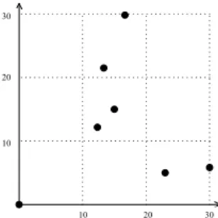
Figure 3: Cutting Node Cube

4.4 Extended Node Bounding

With EMINC, we use bounding technique to filter unnecessary queries. However, EMINC has some limitations and could be fur-ther extended to provide much better performance.

In EMINC, we make one cube for each node to describe the smallest and biggest key value on this node. But under some occa-sions, the performance could still be poor.

Example 3 :Suppose we have two nodes now: data on node A have key value on attribute X from 1 to 100, each integer included; data on node B have only three values, 1, 50 and 100. By the previous approach, node cubes of the two nodes will both be [1,100] on di-mension(attribute) X. And now we have a query asking for records with attribute X between 60 and 80. In the current situation both of the nodes will be selected as candidate since their cubes both intersect with the query cube. But we can easily see that search on node B will end up getting nothing since node B doesn’t hold any record between 60 and 80.

We can see from the extreme case stated in above example that if we use one node cube to describe a node, the cube may be so sparse that it will lead to a great number of waste of searching since sparse distribution on nodes will cause many unrelated queries. To deal with this problem, we propose to extend EMINC to use multiple node cubes to represent a slave node more precisely, and by doing this we will be able to filter out much more irrelevant queries.

In order to achieve higher accuracy, we need to cut the original node cube into several denser smaller cubes, and then adjust the smaller cubes by checking data records within each cube. We name this approachEEMINC: Extended EMINC.

Definition 5. EEMINCis an extension of EMINC. The

differ-ence from EMINC is that in EEMINC data records on one slave node will be represented by multiple node cubes. The shape and amount of node cubes is dependant on the method used for cutting the original single node cube.

Here we give an example on turning the node cube of EMINC into cubes of EEMINC. Discussion on different methods of cutting attributes will be presented later in the section.

Example 4 : Suppose on some node A, we have 7 data records: [0, 0], [12, 12], [15, 15], [13, 21], [17, 30],[23, 5], [30, 6]. See the distribution of data in the coordinate in Figure 3. The node cube of this node is {[0, 30], [0, 30]}. Now we cut both axis X and Y to three equal pieces and get nine small regions. From the distribution of records we can see that only four of the nine regions have records in them, and we only keep those four regions. Now we make four node cubes by checking the actual records within each of the four regions, and what we get are: {[0, 0], [0, 0]}, {[12, 15], [12, 15]}, {[13, 17], [21, 30]}, {[23, 30], [5, 6]}

(6)

In the above example we divided a node cube into nine smaller cubes and picked four of them. The next step is to deliver the cubes to master nodes. After maintaining the new smaller cubes, master nodes can direct queries more accurately. After the reconstruction of node cubes, we turn one sparse cube into several smaller but denser cubes, and that is the key factor of efficiency improvement. With this approach we can further filter out more irrelevant queries in query processing.

Query Processing

The query processing procedure will not present much differ-ence from that in EMINC. The differdiffer-ence lies in the efficiency. With node cubes with better granularity, the chance of forward-ing queries to nodes that don’t have relative records will be greatly diminished.

Index Maintenance

When a new data record needs to be inserted, we first check if it can be enclosed by one of the existing cubes. If we fail to find such cube, we expand the nearest cube to enclose this record. When a record needs to be deleted, we look for the cube it’s in and check if this record is on the vertex of that cube, and if the answer is yes, the node cube shrinks.

However, as the slave node accumulates more and more data up-date operations, node cubes may need to be upup-dated since the data distribution within a node cube may be sparse or uneven again. And when this happens, we shall need to update that node cube to maintain the efficiency. To achieve this we have to answer two questions: when to update the cube and how to reshape the cube ?

We answer the second question first. The reshaping process is similar to the process of cutting the original single cube into several small cubes. The core problem is how to cut each attribute dimen-sion into small intervals. In this paper we try several methods to do the cutting and compare their performances in our evaluation.

• Random cutting. Pick several random value points on the attribute and cut by the points. This cutting method may seems somewhat too "random" to be effective, however, in many occasions the distribution of data also shows certain level of randomness and under that circumstance this method may give good performance, but it is not guaranteed due to the randomness.

• Equal cutting. Cut the attribute into several equal inter-vals. If data insertion operations are controlled by the master in a way that data on each slave node shows approximate hypodispersion, the equal cutting would give good perfor-mance.

• Clustering-based cutting. Cut the attribute by clustering values on the attribute using clustering algorithms and cut be-tween clusters. On some occasions, data records are inserted in a batch way, a transaction for example. So one batch of records may appear to be a cluster and the total records on this node can be seen as a set of clusters. Under this circum-stance, clustering-based cutting method will perform much better than random and equal cutting since it captures the characteristic of data. However, the cost of this method is also higher since a typical clustering algorithms is inO(n2₎ time complexity.

No matter what method is used for cutting, we should stop cut-ting when the total number of nodes cubes reaches a certain amount because the number of cubes should be kept relatively small com-paring to the number of records since large number of cubes will bring down the efficiency of the master nodes.

4.5 Cost Estimation based Update Strategy

Now we go back to the first problem of when to do the reshap-ing of node cubes. As we can see that updatreshap-ing node cubes can give great benefit to query processing, but the cost of updating is also nontrivial since even the fastest cutting method is inO(n) time complexity wherenis the number of data records on this slave node. So when to do the update depends on the comparison of benefit and cost of doing so. So the basic idea is: benefit > cost.

Here we propose a cost-estimation-based approach to handle the cube update problem. First we introduce several concepts and pa-rameters we will need for estimation.

Definition 6. Volumeof a node cube is defined as the maximum

number of unique records that this cube can cover. We note volume of a cube byv.

Example 5 : For the node cube {[1, 11], [2, 5]}, the volume is (11-1)*(5-2) = 30.

To simplify the discussion, we make the following assumption:

Assumption 1. The amount of queries forwarded to each slave

node is proportional to the total volume of all the node cubes of the slave node.

This assumption is reasonable since the bigger is the total vol-ume, the more data records it is likely to hold. Thus more queries are directed to this node. Then we can easily conclude that in the process of reshaping one node cube into one or more smaller cubes, the smaller the total volume of the small cubes is, the better. This also means that the cutting method must be able to decrease the volume otherwise it makes no sense to do the update.

For each node cube, we usenqto denote the number of queries whose query cubes intersect with this cube in each time unit. We can see thatnqdescribes the contribution of this cube to the query load on this node. And from the above assumption we can see that

nqis proportional to the volumevof the cube. We useqtto denote the average time needed to process a query on this node.mtis used to denote the time needed to do a update of cube. Those parameters could be maintained by the cloud platform as metadata.

To make the benefit and cost of update comparable, we express both of them in the metric of number of queries. In other words, we express benefits by how many unrelated queries we can avoid after the update, and express cost by how many queries we could have processed if we use the update time for answering queries.

Benefit of the update can be evaluated by the number of queries that will no longer be forwarded to this node due to this update. And recall that the number of queries is proportional to the volume of cube, so we have:

With the metric of number of query, we express benefit of an update as:

bene f it=(δv/v)×nq×δT (1)

δvrefers to the decrement of volume after the update, soδv/v×nq

means the amount of query that will no longer be forwarded to this node due to this update in one time unit since the amount of query is proportional to the volume. We denote theδv/vas the

benefit ratioof this update since it tells the percentage of queries

this update can save. δT is the time span from now to when next update happens. So the benefit of this update can be measured by how many irrelative queries we can avoid.

The time cost of the whole reshaping procedure consists of two major parts: reshape the cube into one or more cubes and insert the new cubes to the R-tree on master nodes. As we mentioned that the

(7)

number of cubes is kept relatively small. Thus, the cost of inserting them into the R-tree on master nodes will also be neglectable com-paring to the reshaping time which is often at least proportional to the size of data records (we express this trivial cost as). So what we really care is the time cost of reshaping. Using the query number metric, we express cost as:

cost=(mt+)/qt≈mt/qt (2)

We use an iterative two phase approach for the update strategy. After each update, we first calculate a minimal time span before the next update could happen - theδT we introduced. When the time span expires, we calculate the benefit of doing the next update, and if the benefit is acceptable based on several factors, we do the update, and if the benefit is not qualified, we wait anotherδT and check it again.

Substitute formula 2 and 3 into formula 1 we get

(δv/v)×nq×δT >mt/qt (3) Reform formula 4 we have

δT >(mt×v)/(qt×δv×nq) (4) And this is the condition thatδT must meet to ensure the bene-fit. All the parameters concerned could be got from the last update process or maintained by the platform.

And when theδT expires, we have to check each of the descen-dant cube if we need to update them. The reason for this check is highly dependant on several aspects such as amount of data update operation, expected benefit of next update, performance require-ment of the platform and so on.

• Record update frequency. If there has not been many up-date operation since last cube upup-date, we may gain little from another update.

• Expected benefit ratio. Expected benefit ratio refers to the benefit ratio of next update if we do the update now, and it is also calculated based on estimation. For example, if the operations occurred didn’t quite change the distribution of data in the cube, the expected benefit of doing an reshaping will be pretty small.

• Performance requirement. Although we use aδT to as-sure each update being enough utilized, the real time cost of the update process is still inevitable as the update will slow down the real time query processing. So if the performance requirement of the platform is hight, the cube update should not be frequent.

The factors are highly dependant on the specific requirement of the platform and application. We leave the study of combining these factors as future work.

From the discussion we can summarize the process of doing up-date after one upup-date as algorithm 10 :

Now we can see that after the first update of node cube, the index maintenance could continue as we discussed. The only remaining problem is when to perform the first update of node cube. In fact, when to do the first update has high correlation with what we dis-cussed in the checking phase. That is, the environment and require-ment of the application and platform must be carefully studied in order to make the decision. Due to limit of time and length of this paper, we will take this as a future work.

Algorithm 10Deciding next update 1: Time t = calculate minimal time span; 2: wait(t);

3: boolean isToUpdate = check(); 4:

5: while(isToUpdate == false)do

6: wait(t);

7: isToUpdate = check(); 8: end while

9:

10: if(cube number below limit)then

11: updateCube();

12: handle new cubes in R-tree on master nodes; 13: end if

5. EVALUATION

We now evaluate the performance and scalability of our multi-dimensional index in cloud computing systems. Our testing in-frastructure includes 6 machines which are connected together to simulate cloud computing platforms. Communication bandwidth was 1Gps. Each machine had a 2.33GHz Intel Core2 Quad CPU, 4GB of main memory, and a 320G disk. Machines ran Ubuntu 9.04 Server OS.

We use this infrastructure to simulate different sizes of cloud computing systems. We conducted 10 simulation experiments, rang-ing from 100 nodes to 1000 nodes. Each time 100 more nodes are considered to be added into the cloud computing system. In our in-frastructure, one machine plays the role of master nodes and store metadata and control distribution. Each of the other five machines simulates 100 to 1000 slave nodes.

We design two sets of experiments to evaluate our multi-dimensional index’s performance and scalability. One is point query (equiva-lence queries), the other is range query with selectivity being about one ten thousandth. Respectively, we measured the query answer time through using scan, multi-dimensional index with a node cube (EMINC), multi-dimensional index with fine-grained granularity cube(extended EMINC) by random cutting, Equal cutting, K-Means clustering cutting, DBScan clustering cutting. For each experiment, we obtain the result based on 3 runs.

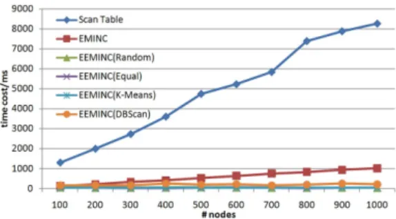
Firstly, we used six methods to execute the point query. Scan method used Map-Reduce functions to scan data on every slave node. EMINC method build a KD-tree on every slave node and construct a node cube for R-Tree on the master node. EEMINC method used several methods to do the cutting. We adopt two clus-tering algorithms: K-Means clusclus-tering and DBScan clusclus-tering. The first is a classical clustering algorithm, and the second is a density based clustering algorithm. These cutting algorithms make bet-ter granularity and improve query processing efficiency. Figure 4 shows the point query experiment result. As can be seen, EM-INC can solve the multi-dimensional query inefficient problem, but EEMINC perform much better than table scan and EMINC. Equal cutting, random cutting and K-Means clustering cutting have simi-lar performance in our dataset. These three methods answered the point query in 1 thousand nodes and 10 million records only cost 40 ∼50 ms, which shows our method is efficient. Figure 4 il-lustrates the scalability of our methods. This graph show that our multi-dimensional distributed index scales almost linearly with the number of nodes in the system.

Secondly, we used six methods to execute the range query. Each query got one ten thousandth of the size of all records. Figure 5 shows the range query experiment result. Compared with the cost of point access, the range query execution time shows that our

(8)

Figure 4: Point Query Experiment Result

multi-dimensional distributed index can also support range query efficiently. And EEMINC method is still the most effective index to answer these queries. Figure 5 shows our methods are high avail-ability and scale to hundreds of nodes.

Figure 5: Range Query Experiment Result

6. CONCLUSION

In this paper we presented EMINC and EEMINC for building efficient multi-dimensional index in Cloud platform. We used the combination of R-tree and KD-tree to support the index structure. We developed the node bounding technique to reduce query pro-cessing cost on the Cloud platform. In order to maintain efficiency of the index, we proposed a cost estimation-based approach for in-dex update. And we proved the efficacy of our approach with vast experiment.

For future work, we will study how to cut node cube according to data distribution in the cube to achieve better performance, both in-dex building performance and query processing performance. We also plan to complete the cost estimation model by formalize the check phase of our two-phase estimation approach. And the ap-proaches we proposed didn’t give much attention to multiple repli-cas of data and left that to the underlying file system, however, if we take that into consideration the efficiency and stability of the index can be further enhanced.

7. ACKNOWLEDGMENTS

The authors thank anonymous reviewers for their constructive comments. This research was partially supported by the grants from 863 National High-Tech Research and Development Plan of China (No: 2007AA01Z155, 2009AA01Z133, 2009AA011904), National Science Foundation of China (NSFC) under the number (No.60833005) and Key Project in Ministry of Education (No: 109004).

8. REFERENCES

[1] Timothy. (2008, July) Multiple experts try defining cloud computing. [Online]. Available:

http://tech.slashdot.org/article.pl?sid=08/07/17/2117221 [2] M. Lynch. Amazon elastic compute cloud (amazon ec2).

[Online]. Available: http://aws.amazon.com/ec2/ [3] IBM. Ibm introduces ready-to-use cloud computing.

[Online]. Available:

http://www-03.ibm.com/press/us/en/pressrelease/22613.wss [4] J. Dean and S. Ghemawat, “Mapreduce: simplified data

processing on large clusters,”Communications of the ACM, vol. 51, pp. 107–113, January 2008.

[5] F. Chang, J. Dean, S. Ghemawat, W. C. Hsieh, D. A. Wallach, M. Burrows, T. Chandra, A. Fikes, and R. Gruber, “Bigtable: A distributed storage system for structured data,”

inProceedings of the 7th Conference on USENIX Symposium

on Operating Systems Design and Implementation, Seattle,

Washington, November 2006, pp. 205–218.

[6] S. Ghemawat, H. Gobioff, and S.-T. Leung, “The google file system,” inProceedings of SOSP’03, New York, USA, December 2003, pp. 29–43.

[7] Hadoop. [Online]. Available: http://hadoop.apache.org [8] M. K. Aguilera, W. Golab, and M. A. Shah, “A practical

scalable distributed b-tree,” inProceedings of VLDB’08, Auckland, New Zealand, August 2008, pp. 598–609. [9] H. chih Yang and D. S. Parker, “Traverse: Simplified

indexing on large map-reduce-merge clusters,” in

Proceedings of DASFAA 2009, Brisbane, Australia, April

2009, pp. 308–322.

[10] M. Aguilera, A. Merchant, M. Shah, A. Veitch, and C. Karamanolis, “Sinfonia: a new paradigm for building scalable distributed systems,” inProceeding of SOSP’07, Washington, USA, October 2007, pp. 159–174.

[11] S. Wu and K.-L. Wu, “An indexing framework for efficient retrieval on the cloud,”IEEE Data Eng. Bull., vol. 32, pp. 75–82, 2009.

[12] T. Johnson and A. Colbrook, “A distributed data-balanced dictionary based on the b-link tree,” inProceeding of

IPPS’92, California, USA, March 1992, pp. 319–324.

[13] J. MacCormick, N. Murphy, M. Najork, C. Thekkath, and L. Zhou, “Boxwood: Abstractions as the foundation for storage infrastructure,” inProceeding of OSDI’04, San Francisco, California, USA, December 2004, pp. 105–120. [14] I. Stoica, R. Morris, D. Karger, F. Kaashoek, and

H. Balakrishnan, “Chord: A scalable peer-to-peer lookup service for internet applications,” inProceedings of

SIGCOMM’01, San Diego, California, USA, August 2001,

pp. 149–160.

[15] S. Ratnasamy, P. Francis, M. Handley, R. Karp, and S. Shenker, “A scalable content-addressable network,” in

Proceedings of SIGCOMM’01, San Diego, California,

United States, August 2001, pp. 161–172.

[16] A. Andrzejak and Z. Xu, “Scalable, efficient range queries for grid information services,” inProceedings of the 2nd International Conference on Peer-to-Peer Computing (P2P

2002), LinkÃ˝uping, Sweden, September 2002, pp. 33–40.

[17] T. K. Sellis, N. Roussopoulos, and C. Faloutsos, “The r -tree: A dynamic index for multi-dimensional objects,” inThe

VLDB Journal, 1987, pp. 507–518.

[18] H. Garcia-Molina, J. D. Ullman, and J. Widom,Database

System Implementation. Upper Saddle River, NJ, USA: