Universit`
a di Pisa
Scuola di dottorato Scienze di base “Galileo Galilei”
Dottorato in fisica
Deterministic
Abelian Sandpile Models
and Patterns
Supervisor:
Prof. Sergio CARACCIOLO
P.A.C.S.: 05.65.bPhD Thesis:
Guglielmo PAOLETTI
Matr. Nr 434802
a Raffaele mio pap´a
Contents
1 Introduction 1
1.1 Shape formation in cellular automata . . . 1
1.2 The many faces of the Abelian Sandpile Model . . . 3
1.3 Overview . . . 4
2 The Abelian Sandpile Model. 7 2.1 General properties . . . 7
2.1.1 Abelian structure . . . 10
2.2 The abelian group . . . 12
2.3 The evolution operator and the steady state . . . 13
2.4 Recurrent and transient configurations . . . 14
2.4.1 The multiplication by identity test . . . 15
2.4.2 Burning test . . . 15
2.5 Algebraic aspects . . . 18
2.5.1 Toppling invariants . . . 18
2.5.2 Rank of G for a rectangular lattice . . . 21
2.6 Generalized toppling rules . . . 22
3 Algebraic structure. 29 3.1 The extended configuration space . . . 29
3.1.1 Algebraic formalism . . . 29
3.1.2 Further aspects of the theory . . . 32
3.2 Statement of results . . . 36
3.2.1 Generalization of Theorem 4 . . . 38
3.3 Multitopplings in Abelian Sandpiles . . . 40
3.4 Wild Orchids . . . 44
4 Identity characterization 47 4.1 Introduction . . . 47
4.1.1 Identity and patterns . . . 47
4.1.2 ASM: some mathematics . . . 47
4.2 Identities . . . 50
4.4 Pseudo-Manhattan Lattice . . . 53
4.5 Proof of the theorem . . . 59
4.6 Manhattan Lattice . . . 62
4.7 Conclusions . . . 64
5 Pattern formation. 67 5.1 Introduction . . . 67
5.2 Experimental protocols for strings and patches . . . 69
5.2.1 Master protocol . . . 70
5.2.2 Wild Orchids . . . 75
5.3 First results . . . 75
5.4 Patches and strings on theZ2 lattice . . . . 79
5.5 Strings construction and vertices . . . 86
5.5.1 Patches from strings . . . 94
5.6 The Sierpi´nski triangle . . . 94
5.6.1 Proof . . . 96
5.6.2 The fundamental Sierpi´nski . . . 101
5.7 Conclusions . . . 102
6 Conclusions 111 A SL(2,Z) 115 A.1 Some simple properties of SL(2,Z) . . . 116
A.2 Modular group Γ . . . 121
B Complex notation for vectors in R2 123 C Generalized quadratic B´ezier curve 125 D Tessellation 129 D.1 Graphics and design . . . 129
D.2 Tiles, tilings and patches . . . 131
D.3 Symmetry, transitivity and regularity . . . 133
D.4 Symmetry groups of tiling: strip group and wallpaper group. . . 136
D.4.1 Crystallographic notation . . . 141
D.4.2 Orbifold notation . . . 142
1.
Introduction
In the last twenty years, after the first article by Bak, Tang and Wiesenfeld [1] on Self-Organized criticality (SOC), a large amount of work has been done trying to better understand different features of this class of models. The most studied among them is theAbelian Sandpile Model (ASM), that was actually proposed as first archetype of SOC in [1], and the attention has been focused mainly on the comprehension of the critical properties, in particular the determination of the critical exponents of the avalanches. During my PhD I worked on the Abelian Sandpile Model using unconventional approaches and focusing on not-standard features of the model, related with the pattern formation that can be seen in the evolution of particularly chosen configurations under deterministic conditions, that happened to catch the attention of the scientific community only in the last few years.
1.1
Shape formation in cellular automata
Since the appearance of the masterpiece by D’Arcy [2], there have been many attempts to understand the complexity and variety of shapes appearing in Nature at macroscopic scales, in terms of the fundamental laws which govern the dynamics at microscopic level. Because of the second law of thermodynamics, the necessary self-organization can emerge only in non-equilibrium statistical mechanics.
In the context of a continuous evolution in a differential manifold, the definition of a shape implies a boundary and thus a discontinuity. This explains why catastrophe theory, the mathematical treatment of continuous actions producing a discontinuous re-sult, has been developed in strict connection to the problem of Morphogenesis [3]. More quantitative results, and modelisations in terms of microscopic dynamics, have been obtained by the introduction of stochasticity, as for example in the diffusion-limited ag-gregation [4, 5, 6, 7], where self-similar patterns with fractal scaling dimension emerge [8], which suggest a relation with scaling studies in non-equilibrium.
Cellular automata, that is, dynamical systems with discretized time, space and inter-nal states, were origiinter-nally introduced by Ulam and von Neumann in the 1940s, and then commonly used as a simplified description of non-equilibrium phenomena like crystal growth, Navier-Stokes equations and transport processes [9]. They often exhibit intrigu-ing patterns and, in this regular discrete settintrigu-ing,shapesrefer to sharply bounded regions in which periodic patterns appear. Despite very simple local evolution rules, very com-plex structures can be generated, and a scale unrelated to the lattice discretization can
be produced spontaneously by the system evolution. The well-known Conway’s Game of Life, which can even emulate an universal Turing machine, is an example of this emerg-ing complexity, but a detailed characterization of such structures is usually not easy (see [10, 11], also for a historical introduction on cellular automata).
Cellular automata are defined through a set of configurations and an intrinsic evo-lution law, and a given automaton may be studied under different evoevo-lution dynamics. These dynamics may be roughly divided into two classes: stochastic and deterministic
ones. As emphasized above, it is the ingredient of stochasticity that, in parallel to what emerges in critical phenomena for non-equilibrium statistical mechanics, suggests the possibility of obtaining probability laws which are “scale-free”, that is, in which correla-tions among different spatially-separated parts do not decrease exponentially, at a scale related to the lattice discretization, but instead have an algebraic decay.
In equilibrium statistical mechanics, we expect criticality only at a fine-tuned value of a thermodynamic parameter (e.g., the temperature), if we have spontaneous symmetry breaking of a discrete group, and criticality for a subset of the degrees of freedom, in the whole ordered phase, if we have a continuous group and Goldstone bosons. In non-equilibrium systems the theoretical picture is less clear. Apparently, the non-non-equilibrium ingredient has often the tendency of increasing the scale-free region of parameters, or even automatically set the system in a scale-free point, without tuning of parameters, possibly by making all the “mass” operators irrelevant under the flow of the Renormalization Group (while, for equilibrium systems having a “magnetic” order parameter m, the temperature T and external field h always correspond to relevant operators). Such a feature is called Self-Organized Criticality.
A further feature of lattice automata is the possibility of producingallometry, that is a growth uniform and constant in all the parts of a pattern as to keep the whole shape substantially unchanged. Such a feature requires some coordination and communication between different parts, and is thus at variance with diffusion-limited aggregation and other models of growing objects studied in physics literature so far, e.g. the Eden model, KPZ deposition and invasion-percolation [12, 13, 14], which are mainly models of aggre-gation, where growth occurs by accretion on the surface of the object, and inner parts do not evolve significantly. The lattice automaton discussed in [15], where this feature is discussed and outlined very clearly through an explicit model realization, is indeed a variant of theAbelian Sandpile Model, the general class of models that we will investigate in this thesis.
Another distinguished property of automata is that allometry emerges from a deter-ministic dynamics of the automaton, and thus we do not have a theoretical explanation in terms of stochastic processes, and steady-state distributions solving the master equation associated to a Markov chain. The theoretical approach followed in [15] is to investi-gate, at a coarse-grained level, the properties of what we may call a discrete-valued Heat Equation, strictly related to the intrinsic evolution law of the automaton (and not to the dynamics).
While the ordinary massless Heat Equation, formally solved within the realm of linear algebra, is automatically scale-free, the discretization in target space, and its counterpart, which is allowing for a tolerance offset in the resulting vector, produces a non-linearity.
1.2 The many faces of the Abelian Sandpile Model 3
It is the interplay of these two ingredients that ultimately allows to have non-trivial shapes (through the non-trivial effects of non-linearity), on extended regions (through the absence of scale caused by the linear Heat Equation at leading order).
This phenomenology — of introducing a “small” non-linearity, through discretization, in a classical real-valued scale-free equation, and analyzing the possible emergence of morphogenesis — has a possibility of being realized in other models besides the Abelian Sandpile. Note however a subtlety here: in order to have a well-posed problem, it is crucial to find a discretization that preserves the unicity of the solution. In the case of the ASM, this relies on a non-trivial property of the model, namely, the unicity of the relaxation process, and ultimately the “abelianity” of the sandpile, that allows to perform a single relaxation in place of a sequence of maps in a non-commutative monoid, as is the case for a generic automaton.
1.2
The many faces of the Abelian Sandpile Model
As anticipated in the first paragraph, in this thesis we will concentrate on a particularly simple cellular automaton, theAbelian Sandpile Model (ASM). This model, now existing since about 20 years, was first proposed by Bak, Tang and Wiesenfeld in [1]. It has shown to be ubiquitous, as a toy model for a variety of features in Physics, Mathematics and Computer Science, including but not restricted to the ones described in the section above.
As all cellular automata, it has an intrinsic evolution law, and may be studied un-der different dynamics. These dynamics may be roughly divided into stochastic and
deterministic ones. Thus we address explicit studies of the ASM under stochastic or deterministic dynamics as theStochastic Abelian Sandpile and theDeterministic Abelian Sandpile respectively. We will give particular importance to the deterministic dynam-ics in the sandpile, although some particular stochastic dynamdynam-ics will be part of the discussion.
The Stochastic Abelian Sandpile has been the first variant studied in physics litera-ture. It is in this framework that it was proposed in the work of Bak, Tang and Wiesenfeld as first example of a model showing SOC1 in 1987 because it shows scaling laws
with-out any fine-tuning of an external control parameter. this article has truly triggered an avalanche. Indeed a huge number of articles has been published on SOC, the BTW article alone collected 1924 citations2. With the aim of determine the critical exponents
of the model a great work has been done collecting statistics of the model under stochas-tic evolution, see [17]. Just a few years later,thanks to the work of Dhar, the algebraic properties of the sandpile were pointed out in [18, 19], where he first elucidated the group structure underlying the model, that allows to determine the statistic of the Recurrent configurations of the model, that happens to be uniform. In a subsequent work together in collaboration with Ruelle et.al. [20] Dhar dealt in deep with the algebraic aspects of
1A good introductory reading on Self Organized Criticality is the bookHow nature works[16] by Bak, which underlines the ubiquitous of SOC in nature, social sciences, economics and many other fields.
the sandpile, introducing some useful methods to determine the Smith normal form of the group.
The model was then studied by Creutz [21, 22], he was the first “looking” at the configurations and thus noting the particular and interesting shapes emerging in the identity configuration. He observed in particular how this configuration seemed to display self-similarity and a fractal structure [23, 24].
Afterwards the height correlation of the model has been widely studied in a number of papers [25, 26, 27]. A connection with conformal Field theory came first when the equivalence of the ASM with the q→0 limit of theq-state Potts Model was established [28]; thus two-dimensional ASM corresponds to a conformal field theory with central charge c=−2. This equivalence gives also a Monte Carlo algorithm to generate random spanning trees. Connections between ASM and the underlying CFT theory have been further studied by Ruelleet.al. in [29, 30, 31, 32, 33] and then more recently in [34, 35, 36, 37].
The connection with uniform spanning trees and the Kirchhoff theorem explains a posteriori the arising of self-organized criticality, i.e. the appearance of long-range be-havior with no need of tuning any parameter. Indeed, uniform spanning trees on reg-ular 2-dimensional lattices are ac =−2 logarithmic Conformal Field Theory (CFT) in [30], and have no parameter at all, being a peculiar limit q → 0 of the Potts model in Fortuin-Kasteleyn formulation [38], or a limit of zero curvature in the OSP(1|2) non-linear σ-model [39]. If instead one considers the larger ensemble of spanning forests, in a parameter t counting the components (or describing the curvature of the OSP(1|2) supersphere), the theory in two dimensions is scale-invariant for three values: att = 0 (the spanning trees, or the endpoint of the ferromagnetic critical line of Potts), at the infinite-temperature point t = ∞, and at some non-universal negative t corresponding to the endpoint of the anti-ferromagnetic critical line of Potts, being tc =−1/4 on the
square lattice. Through the correspondence with the non-linear σ-model, one can deduce at a perturbative level that the system is asymptotically free at t = 0+, i.e. that the “coarse-graining” of a system with parameter t > 0, by a given scale factor Λ, “looks like” a system at parametert′ > t, but the functional dependence of ln t′(t; Λ)/t is only quadratic in tfort→0, instead of linear, as in the generic case [39, 40].
The Deterministic Abelian Sandpile Model, especially at earlier times, has been stud-ied in Mathematics and computer-science literature under the name ofChip-Firing Game
[41, 42]. A particularly interesting result of chip-firing game in connection with tutte polynomials has been obtained by Merino in [43], allowing to determine properties of the recurrent configurations of the model.
1.3
Overview
As anticipated in section 1.1, in this thesis we want to study the ASM in connection with its capability to produce interesting patterns. it is a surprising example of model that shows the emergence of patterns but maintains the property of being analytically tractable. Then it is qualitatively different from other typical growth models –like Eden
1.3 Overview 5
model, the diffusion limit aggregation, or the surface deposition [13, 4, 14]– indeed while in these models the growth of the patterns is confined on the surfaces and the inner structures, once formed, are frozen and do not evolve anymore, in the ASM the patterns formed grow in size but at the same time the internal structures aquire structure, as it has been noted in [15, 44, 45, 46].
There have been several earlier studies of the spatial patterns in sandpile models. The first of them was by Liu et.al. [47]. The asymptotic shape of the boundaries of the patterns produced in centrally seeded sandpile model on different periodic backgrounds was discussed in [48]. Borgne et.al. [49] obtained bounds on the rate of growth of these boundaries, and later these bounds were improved by Fey et.al. [50] and Levine
et.al. [51]. An analysis of different periodic structures found in the patterns were first carriedout by Ostojic [52] who also first noted the exact quadratic nature of the toppling function within a patch. Wilson et.al. [53] have developed a very efficient algorithm to generate patterns for a large numbers of particles added, which allows them to generate pictures of patterns with N up to 226.
There are other models, which are related to the Abelian Sandpile Model, e.g., the Internal Diffusion-Limited Aggregation (IDLA) [54], Eulerian walkers (also called the rotor-router model) [55, 56, 57], and the infinitely-divisible sandpile [51], which also show similar structure. For the IDLA, Gravner and Quastel showed that the asymptotic shape of the growth pattern is related to the classical Stefan problem in hydrodynamics, and determined the exact radius of the pattern with a single point source [58]. Levine and Peres have studied patterns with multiple sources in these models, and proved the existence of a limit shape[59]. Limiting shapes for the non-Abelian sandpile has recently been studied by Fey et.al. [60].
The results of our investigation toward a comprehension of the patterns emerging in the ASM are reported along the thesis.
In chapter 3 we will introduce some new algebraic operators, a†i and Πi in addition
to ai, over the space of the sandpile configurations, that will be in the following basic
ingredients in the creation of patterns in the sandpile. We derive some Temperley-Lieb like relations they satisfy. At the end of the chapter we show how do they are closely related to multitopplings and which consequences has that relation on the action of Πi
on recurrent configurations.
In chapter 4 we search for a closed formula to characterize the Identity configuration of the ASM. At this scope we study the ASM on the square lattice, in different geometries, and in a variant with directed edges, theF-latticeorpseudo-Manhattan lattice. Cylinders, through their extra symmetry, allow an easy characterization of the identity which is a homogeneous function. In the directed version, the pseudo-Manhattan lattice, we see a remarkable exact self-similar structure at different sizes, which results in the possibility to give a closed formula for the identity, this work has been published in [61]
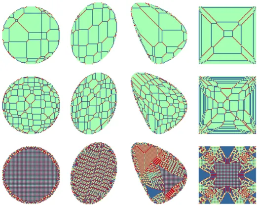
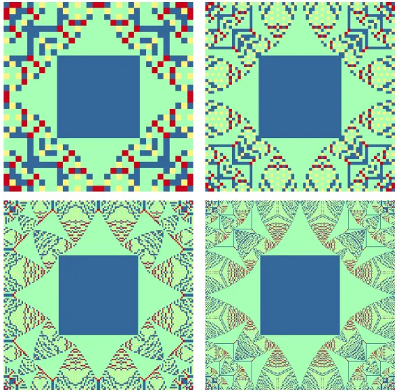
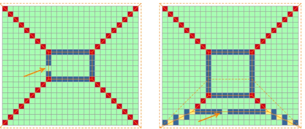
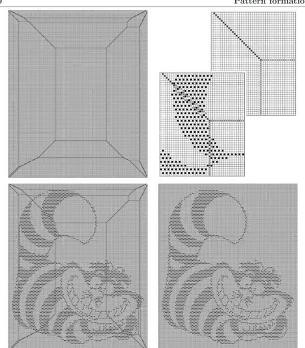
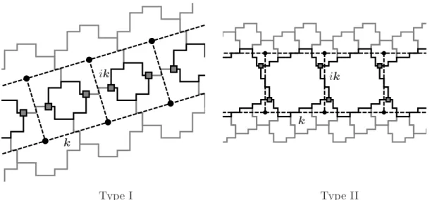
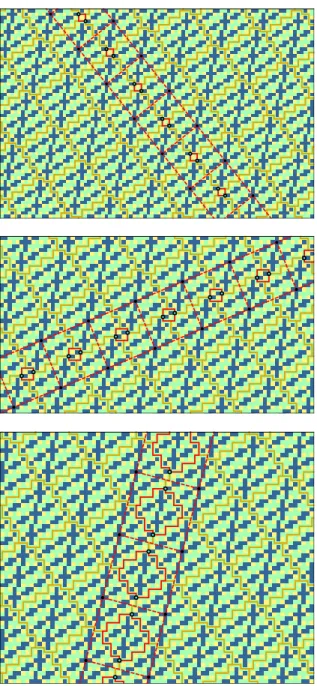
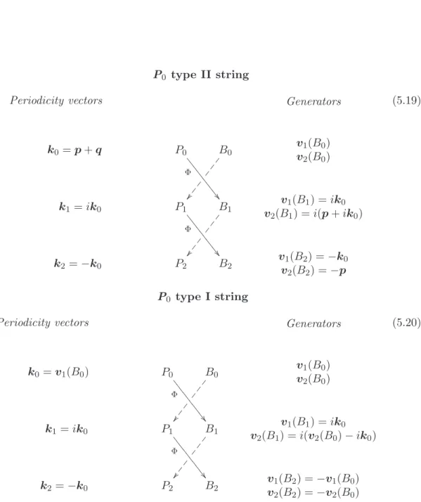
In chapter 5 we reach the cardinal point of our study, here we present the theory of strings and patches. The regions of a configuration periodic in space, called patches, are the ingredients of pattern formation. In [15], a condition on the shape of patch interfaces has been established, and proven at a coarse-grained level. We discuss how
this result is strengthened by avoiding the coarsening, and describe the emerging fine-level structures, including linear interfaces and rigid domain walls with a residual one-dimensional translational invariance. These structures, that we shall call strings, are macroscopically extended in their periodic direction, while showing thickness in a full range of scales between the microscopic lattice spacing and the macroscopic volume size. We first explore the relations among these objects and then we present full classification of them, which leads to the construction and explanation of aSierpi´ski triangular structure, which displays patterns of all the possible patches.
2.
The Abelian Sandpile Model.
The state of the art
It has been more than 20 years since Bak, Tang and Wiesenfeld’s landmark papers on self-organized criticality (SOC) appeared [1]. The concept of self-organized criticality has been invoked to describe a large variety of different systems. We shall describe the model object of our interest: the Abelian Sandpile Model (ASM). The sandpile model was first proposed as a paradigm of SOC and it is certainly the simplest, and best understood, theoretical model of SOC: it is a non-equilibrium system, driven at a slow steady rate, with local threshold relaxation rules, which shows in the steady state relaxation events in bursts of a wide range of sizes, and long-range spatio-temporal correlations. The ASM consists of a special subclass of the sandpile models that exhibits, in the way we will discuss later, the mathematical structure of an abelian group, and its statistics is connected to that of spanning trees on the relative graph. There are a number of review articles on this subject, taking into account the connection of the model with the theme of SOC and its inner mathematical properties: Dhar [62], Priezzhev [63] and Redig[64, 65]. Here we present a review of the Sandpile Model theory based on the material than can be found therein with particular emphasis on mathematical aspects and on its stochastic dynamics; some further development given by us complete the review. This material will be necessary for the comprehension of the studies we discuss in the following chapters.
2.1
General properties
The ASM is defined as follows [18, 62]: we consider any (directed) graph G = (V, E) with |V| = N and vertices labeled by integers i = 1, . . . , N, at each site we define a nonnegative integer height variable zi, called the height of the sandpile, and a threshold
value ¯zi ∈ N+. We define an allowed configuration of the sandpile as a set z ∈ NN
of integer heights z = {zi}i∈V such that zi ≥ 0 ∀i ∈ V; an allowed configuration {zi}
is said to be stable if zi < z¯i ∀i ∈ V. Therefore the set S of stable configurations is
S = Ni∈V{0, . . . ,z¯i}. If we call S± ⊂ Zn the sets respectively such that zi ≥0 for all
i∈V, and zi <z¯i for alli∈V. ThenS+ is te set ofallowed configurations and isstable
if it is in S :=S+∩S−. The involution zi →z¯i−zi−1 exchanges S+ and S−.
The stochastic time evolution of the sandpile is defined in term of thetoppling matrix
1. Adding a particle: Select one of the sites randomly, the probability that the site
i is picked being some given value pi, and add a grain of sand there. Obviously
P
ipi= 1. On addition of the grain at site i,zi increases by 1, while the height at
the other sites remains unchanged.
2. Toppling: If for any site i it happens that zi ≥ z¯i, then the site is said to be
unstable, it topples, and lose some sand grains to other sites. This sand grain’s transfer is defined in terms of an N ×N integer valued toppling matrix ∆, which properties will be specified in (2.2). On toppling at site i, the configuration z is updated globally according to the rule:
zj →zj−∆ij ∀j∈V (2.1)
If the toppling results in some other sites becoming unstable, they are also toppled simultaneously (it will be clear in the following that the order of toppling is unim-portant). The process continues until all sites become stable1 (we will see later under which conditions on the set of threshold values and ∆ the final stability is guaranteed)
At each time step of the stochastic evolution, we first add a particle, as specified in rule 1, then we relax the configuration, that means to perform the necessary topplings to reach a stable configuration as stated in rule 2.
The toppling matrix ∆ has the following properties:
∆ii>0, ∀i∈V (2.2a)
∆ij ≤0, ∀i6=j (2.2b)
b−i :=X
j
∆ij ≥0, ∀i (2.2c)
For future convenience we also define the integers
b+i := X
j∈V
∆Tij ≥0 (2.3)
for any vertex i.
We will adopt a vector notation for the collection of elements ∆~i = {∆ij}j=1,...,N.
With this notation it is possible to rewrite the toppling rule (2.1) for the toppling at site
i as
z→z−∆~i (2.4)
These conditions just ensure that on toppling at site i, zi must decrease, height at
other sites j can only increase and there is no creation of sand in the toppling process. In some sites could be possible to lose some sand during a toppling.
If the graphGis undirected, the toppling matrix ∆ is symmetric andb−i =b+i =bi.
2.1 General properties 9
Figure 2.1 A graphical representation of the general ASM. Each node denotes a site. On topplings at any site, one particle is transferred along each arrow directed outward from the site, each arrow corresponding to a unit in−∆ij.
The graph, in general directed and with multiple edges, is thus identified by the non-diagonal part of −∆, seen as an adjacency matrix, while the non-zero values b±i are regarded as (in- or out-coming) connections to the border, and the sites i with nonzero
b±i are said to beon the border, see fig. 2.1. In particular,b−i is the total sand lost in the toppling process on i, so that, pictorially, we can think of thislost sand as dropping out of some boundary. Clearly, in the formulation on an arbitrary graph, as presented here, this concept of boundary does not need to correspond to any geometrical structure. We note that no stationary state of the sandpile is possible unless the particles can leave the system.
As an example, the original BTW model [1] is defined on an undirected graph which is a rectangular domain of the Z2 lattice. We have in this case
∆ij = +4 ifi=j −1 ifi, j are nearest-neighbors 0 otherwise (2.5)
In this case the connections with the border are given, on the sides of the rectangle, by
bi = 1, while on the corners bybi = 2. In this framework to be on the boundary (or in a
corner) has a direct correspondence with the geometrical structure of the lattice.
We assume, without loss of generality, that ¯zi = ∆ii (this amounts to a particular
choice of the origin of the zi variables). Then we know that if a siteiis stable, and the
initial conditions for the heights are zi(t= 0)≥0∀i∈V, at all times the allowed values
for zi are the ones for which holds 0 ≤ zi < z¯i. This procedure define a Markov chain
on the space of stable configurations, with a given equilibrium measure. So running the stochastic dynamics for long times, that means after a large amount of sand added, the system reaches the stationary state.
As stated in rule 2, if a configuration isunstable which is if there is at least a vertex
iwhere the configuration z has zi ≥ z¯i, the vertex i topples and the configuration z is
updated following the rule 2.4. The new configuration reached after a toppling at site i
is tiz=z−∆~i, where we callti the toppling operator at site i.
The collection of topplings needed to produce a stable configuration is called an
avalanche. We shall assume that an avalanche always stops after a finite number of steps, which is to say that the diffusion is strictlydissipative. The size of avalanches can be studied statistically for interesting graphs (e.g. for a partition of Z2). In many cases
of interest it seems to have a power law tail, which is signal of existence of long-range correlations in the system, see [17].
We shall denote byR(z) the stable configuration obtained from the relaxation of the configuration z, soR(z) ∈S and
z∈S ⇔ z=R(z). (2.6)
Given two configurationsz andw we introduce the configurationz+w which has at each vertexithe heightzi+wi. Calle(i)the configuration which has non-vanishing height
only at the site iwhere it has height 1, that ise(ji)=δij. Of course each configuration z
can be obtained by deposing zi particles at the vertexi
zie(i)=|e(i)+e(i){z+· · ·+e(i}) zi
(2.7)
so that summing on every vertex i, this means
z=X
i∈V
zie(i). (2.8)
2.1.1 Abelian structure
Let ˆai be the operator which adds a particle at the vertex i
ˆ
aiz:=z+e(i) (2.9)
then ifz is not stable at the vertexj,
tjˆaiz= ˆaitjz (2.10)
is easily verified.
Let now ai be the addition of a particle at the vertex i followed by a sequence of
topplings which makes the configuration stable. The stable configuration
aiz=R(e(i)+z) (2.11)
is independent from the sequence of topplings, because topplings commute. Indeed, the final configuration of a sequence of topplings does not depend from the order of unstable vertices chosen for each intermediate toppling. For this reason the model is said to be
2.1 General properties 11
abelian sandpile ASM. More precisely, if the configuration z is such that zi > z¯i and
zj >z¯j then
titjz=tjtiz (2.12)
can be easily verified. Let us consider an unstable configuration with two unstable sites
α and β, toppling first the site α leaves β unstable thanks to (2.2b), and, after the toppling of β, we get a configuration in which z → z−(∆~α +∆~β) this expression is
clearly symmetrical under exchange ofαandβ. Thus we get the same final configuration irrespective of whether α orβ is toppled first. By repeated use of this argument we see that, in an avalanche, the same final state is reached irrespective of the sequence chosen for the unstable sites to topple. similar reasoning apply for toppling of a site α followed by addition of a sand grain in β, so this gives the same result of the reverse ordered operation.
It is clear now that applying two operators ai and aj the configurations ajaiz and
aiajz coincide
aiajz=ajaiz=R(e(i)+e(j)+z) (2.13)
so that ai and aj do commute, or in other word
[ai, aj] = 0 ∀i, j∈V (2.14)
Note that, while this property seems very general, it is not shared with most of the other SOC models, even other sandpile models, for example when the toppling condition de-pends on the gradient, in this case the order of toppling would matter, being the toppling rule not local and dependent on the actual height’s values of the whole configuration.
Given two configurationszand z′ we define an abelian composition z⊕z′ as the sum of the local height variables, followed by a relaxation process
z⊕z′ =R(z+z′) = Y i∈V azi i ! z′ = Y i∈V azi′ i ! z (2.15)
and thus, for a configuration z, we define multiplication by a positive integerk∈N:
k z =z⊕ · · · ⊕z
| {z }
k
(2.16)
The operatorsai’s have some interesting properties. For example, on a square lattice,
when 4 grains are added at a given site, this is forced to topple once and a grain is added to each of his neighbors. Thus:
a4j =aj1aj2aj3aj4 (2.17)
where j1, j2, j3, j4 are the nearest-neighbors of j.
In the general case one has, instead of (2.17),
a∆ii i = Y j6=i a−∆ij j . (2.18)
action of a1
action of a2 action ofai action ofaj
Figure 2.2 graphical representation of the combined action ofai andaj.
by definition, because if we add ¯zi particles at the vertex i, after its toppling these
particles move on the nearest-neighbor vertices, and, since now on, the relaxation to the stable configuration will be identical. Using the abelian property, in any product of operators ai, we can collect together occurrences of the same operator , and using the
reduction rule (2.18), it is possible to reduce the power of ai to be always less than ∆ii.
Theaiare therefore the generators of a finite abelian semi-group (in which the associative
property follow from their definition) subject to the relation (2.18); these relations define completely the semi-group.
Let now consider the repeated action of some given operatoraion some configuration
C. Since the number of possible states is finite, the orbit of ai must close on itself, at
some stage, so thatani+pC =an
iC for some positive periodp, and non negative integern.
The first configuration that occurs twice in the orbit is not necessary C, so that the orbit consists of a sequence of transient configurations, followed by a cycle. If this orbit does not exhaust all configurations, we can take a configuration outside this orbit and repeat the process. So the space of all configurations is broken up into disconnected parts, each one containing one limit cycle.
Under the action ofai the transient configurations are unattainable once the system
has reached one of the periodic configurations. In principle the recurrent configurations might still be reachable as a result of the action of some other operator, say aj, but
the abelian property implies that if C is a configuration part of one of the limit cycles of ai, then so is ajC, in fact apiC = C implies that a
p
iajC = ajapiC = ajC. Thus the
transient configurations with respect to an operator a1 are also transient with respect
to the other operators aj1, aj2, . . ., and hence occur with zero probability in the steady
state. The abelian property thus implies that aj maps the cycles ofai into cycles of ai,
and moreover that all this cycles have the same period fig. 2.2. Repeating our previous argument we can show that the action of aj on a cycle is finally closed on itself to yield
a torus, possibly with some transient cycles, which may be also discarded. Continuing with the same arguments for the other cycles and other generators leads to the conclusion that the set of all the configurations in the various cycles form a set of multi-dimensional tori under the action of the a’s.
2.2 The abelian group 13
if we allow addition of sand with non zero probability in any site (pi > 0 ∀i), as the
configurations reachable by any other configuration with addition of sand followed by relaxation. We denote the set of all recurrent configurations as R.
Given the natural partial ordering, C 4C′ iff zi ≤zi′ for all i, then R is in a sense
“higher” than T, more precisely
∄ (C, C′)∈T×R : C ≻C′; (2.19)
∀C∈T ∃C′ ∈R : C ≺C′. (2.20)
In particular, the maximally-filled configuration Cmax ≡ zmax = {z¯i −1} is in R, and
higher than any other stable configuration.
2.2
The abelian group
The set R of recurrent configurations is special. Indeed in Rit is possible to define the inverse operator a−i 1 for alli, as each configuration in a cycle has exactly one incoming arrow corresponding to the operator ai. Thus the ai operators generate a group. The
action of theai’s on the states correspond to translations of the torus. From the symmetry
of the torus under translations, it is clear that all recurrent states occur in the steady state with the same probability.
This analysis, which is valid for every finite abelian group, leaves open the possibility that some recurrent configurations are not reachable from each other, in which case there would be some mutually disconnected tori. However, such a situation cannot happen if we allow addition of sand at all sites with non zero probabilities (pi>0∀i). Let us define
zmax as the configuration in which all sites have their maximal height,zi = ∆ii−1 ∀i.
The configurationzmaxis reachable from every other configuration, is therefore recurrent,
and since inverses ai’s exist for configurations inR, every configuration is reachable from
zmax implying that every configuration lie in the same torus.
LetG be the group generated by operators{ai}i=1,...,N. This is a finite group because
the operators ai’s, due to (2.18), satisfy the closure relation: N
Y
i=1
a∆ji
i =I ∀i= 1, . . . , N (2.21)
the order of G, denoted as |G|, is equal to the number of recurrent configurations. This is a consequence of the fact that if C and C′ are any two recurrent configurations, then
there is an element g∈ G such thatC′ =gC. We thus have:
|G|=|R| (2.22)
Given the group structure, the semi-group operation (2.15) is raised to a group op-eration, in particular the composition of whatever z with the setRacts as a translation on this toroidal geometry. A further consequence is that, for any recurrent configuration
The identity of this abelian group, denoted by Idr, is called recurrent identity or
Creutz identity after Creutz first studies in [22, 21] and is the only stable recurrent configuration such that
∀z∈R Idr⊕z=z (2.23)
2.3
The evolution operator and the steady state
We consider a vector spaceV whose basis vectors are the different configurations ofR.
The state of the system at time twill be given by a vector
|P(t)i=X
C
Prob(C, t)|Ci , (2.24)
where Prob(C, t) is the probability that the system is in the configuration C at time t. The operators ai can be defined to act on the vector spaceV through their operation on
the basis vectors.
The time evolution is Markovian, and governed by the equation
|P(t+ 1)i=W |P(t)i (2.25) where W = N X i=1 piai (2.26)
To solve the time evolution in general, we have to diagonalize the evolution operator
W. Being mutually commuting, the ai may be simultaneously diagonalized, and this
also diagonalizes W. Let|{φ}i be the simultaneous eigenvector of{ai}, with eigenvalues
{eiφi}, fori= 1, . . . N. Then
ai
{φ}=eiφi{φ} ∀i= 1, . . . , N. (2.27)
We recall that the a operators now satisfy the relation (2.21). Applying the l.h.s. of this relation to the eigenvector |{φ}i gives exp(iPj∆kjφj) = 1, for every k, so that
P j∆kjφj = 2πmk, or inverting, φj = 2π X k ∆−1jkmk , (2.28)
where ∆−1 is the inverse of ∆, and them
k’s are arbitrary integers.
The particular eigenstate |{0}i (φj = 0 for all j) is invariant under the action of all
the a’s,ai|{0}i=|{0}i. Thus|{0}i must be the stationary state of the system since
X i piai|{0}i= X i pi|{0}i =|{0}i . (2.29)
We now see explicitly that the steady state is independent of the values of the pi’s
2.4 Recurrent and transient configurations 15
2.4
Recurrent and transient configurations
Given a stable configuration of the sandpile, how can we distinguish between transient and recurrent configurations? A first observation is that there are some forbidden sub-configuration that can never be created by addiction of sand and relaxation, if not already present in the initial state. The simplest example on the square lattice case is a config-uration with two adjacent sites of height 0, 0 0 . Since zi ≥0, a site of height 0 can
only be created as a result of toppling at one of the two sites (toppling from anywhere else can only increase his height). But a toppling of either of this sites results in a height of at least 1 in the other. Thus any configuration which contains two adjacent 0’s is transient. With the same argument it is easy to prove that the following configurations can never appear in a recurrent configuration:
0
0 0 0 0 1 0 0 3 0
Figure 2.3 Examples of forbidden subconfigurations
In general aforbidden subconfiguration (FSC) is a setF ofr sites (r ≥1), such that the heightzj of each site jinF is less of the number of neighbors thanj inF, precisely:
zi <
X
j∈Fr{i}
(−∆ij) ∀i∈F (2.30)
The proof of this assertion is by induction on the number of sites in F. For example the creation of the 0 1 0 subconfiguration must involve toppling at one of end sites, but then the subconfiguration must have had a 0 0 before the toppling, and this was shown before to be forbidden.
An interesting consequence of the existence of forbidden configurations is the follow-ing: consider an ASM on an undirected graph, with Nb bonds between sites, then in any
recurrent configuration the number of sand grains is greater or equal toNb. Here we do
not count the boundary bonds, corresponding to particles leaving the system. To prove this, we note that if the inequality is not true for any configuration, it must have a FSC in it.
2.4.1 The multiplication by identity test
Consider the product over sites iof equations (2.17)
Y i a∆ii i = Y i Y j6=i a−∆ij j = Y i a− P j6=i∆ji i (2.31)
On the setR, the inverses of the formal operatorsaiare defined, so that we can simplify
common factors in (2.31), recognize the expression for b+i , and get
Y i ab + i i =I (2.32) so thatQiab+i
i z=zis a necessary condition forz to be recurrent (but it is also
suffi-cient, as no transient configuration is found twice in the same realization of the Markov chain), and goes under the name of identity test. If we denote by b+ the configuration
b+=X
i∈V
b+i e(i) (2.33)
the identity test means that
z∈R⇔z=z⊕b+ (2.34)
In the next section we will see how to obtain the same result in an easier and faster way, without actually perform the composition.
This relation gives information also on the recurrent identity itself. Indeed it says that if b+∈Rthenb+ =Idr. Otherwise there must be a positive integerksuch that
∀ℓ∈N:ℓ≥k b+⊕b+⊕ · · · ⊕b+ | {z } ℓ =Idr (2.35) then Idr=kb+. (2.36) 2.4.2 Burning test
There is a simple recursive procedure to discover if a configuration is recurrent, checking mechanically if it has any FSC. We consider at each step a test set, say T, of sites. In the beginning T consists of all the sites of the lattice we are considering; we first test the hypothesis thatT is a FSC using the inequalities (2.30). If these inequalities are satisfied for all sites in T, then the hypothesis is true, T has a FSC, and the configuration in exam is transient. Otherwise there are some sites for which the inequalities are violated, these sites cannot be part of any FSC, in fact the inequalities will remain unsatisfied even thoughT is replaced by a smaller subset of sites. We delete these sites fromT and we have a new subset T′, we say weburn these sites while the remaining areunburnt; at this point we repeat the procedure to check whether T′ is a FSC. We follow this scheme
until we cannot burn anymore site. If we we are left with a finite subset F of unburnt sites this is a FSC and the configuration is transient, if the set of unburnt sites eventually becomes empty the configuration in exam is found to be recurrent. We call the procedure just presented the burning test.
In theburning test it does not matter in which order the sites are burnt. It is however useful to introduce the concept of time of burning and to add to the graph a site, named
2.4 Recurrent and transient configurations 17
of lost particles in a toppling by the boundary sites in exam, it never topples and only collects sand. There is a natural way to choose a time of burning for each site. At time
t= 0, all the sites inT(0) =T are unburnt except the sink. At any timet a site is called
burnable iff the inequality (2.30) is unsatisfied with respect to the setT(t)reached at that time, then a burnable site at time tbecomes burnt at timet+ 1, and so remains for the successive times. With this prescription we label each site of the graph with a burning time, depending just on the configuration in exam.
We want now to draw a path for the “fire” to propagate to the whole graph, starting from the sink. Take an arbitrary site i, except the sink. Let τi + 1 be the time step
at which this is burnt, then the burning rule implies that at time τi at least one of his
neighbor sites has been burnt. Let ri be the number of such neighbors and let us write:
ξi = ri
X′
j=1
(−∆ij) (2.37)
where the primed summation runs over all unburnt neighbors of iat time τi. Then we
have zi ≥ξi since the siteiis burnable at timeτi; but, since it was not burnable at time
τi−1 we must also have:
zi< ξi+K (2.38)
where K is the number of bonds linking ito his neighbors which were unburnt at time
τi. During the burning test we say that fire reaches the site i by one of the K bonds.
Obviously whenK = 1 there is just one possibility so there are no problems, and we say that the fire reaches ifrom the only site possible. If K >1 we have to select one bond through which the fire reaches idepending on his height zi. For this purpose we order
the bonds converging on the site iin some sequence (e.g. {(i, i1),(i, i2),(i, i3), . . .}), the
order is arbitrary and can be chosen independently on each site i. Now we can write
zi =ξi+s−1 for somes >0, we say that fire reaches iusing thes-th link in the ordered
list of the possible ones. This procedure gives a unique path for the fire to reach each sitei, given the configuration of heights in the sandpile and the prescription on the order of bonds converging on each site. The set of bonds along which fire propagates, connects the sink with each site in the graph, and there are no loops in each path. Thus the set just obtained is a spanning tree on the graphG′ =G+{sink}.
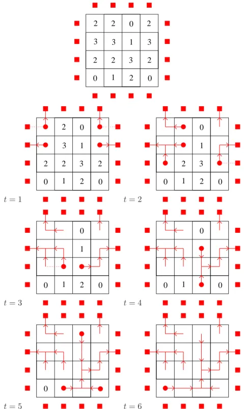
So choosing a particular prescription for a given graph we can obtain for each config-uration a unique spanning tree. For example on a square lattice we have four bonds for each site, let us call them N-E-S-W, where the cardinal points denotes the direction of incidence, we can choose the prescription N>E>S>W and obtain for a recurrent config-uration the corresponding spanning tree. In fig. 2.4 is shown a burning test for a 4×4 square lattice, with prescription NESW, with 00
1
1are denoted the sites such that,
con-nected together, represent the sink, with 000 1 1 1
the sites burnt at the given time of each step of the algorithm and with , the bonds through which the fire could have reached the site but were rejected.
Let us note a few facts about the burning test before going on to the next section. Although all recurrent configurations were shown in [18] to pass the burning test; con-versely, it was shown in [28] only for sandpiles with symmetric toppling rules –which is
0 0 0 2 2 2 2 2 2 1 1 3 3 3 3 2 0 0 1 1 0 0 1 1 0 0 1 1 0 0 0 1 1 1 0 0 0 1 1 1 00 00 00 11 11 11 00 00 00 11 11 11 00 00 11 11 00 00 11 11 00 00 11 11 00 00 00 11 11 11 00 00 00 11 11 11 00 00 00 11 11 11 0 0 0 1 1 1 0 0 0 1 1 1 0 0 0 1 1 1 t= 1 00 00 00 11 11 11 00 00 00 11 11 11 0 0 0 1 1 1 0 0 0 1 1 1 00 00 00 11 11 11 00 00 00 11 11 11 00 00 00 11 11 11 00 00 11 11 0 0 1 1 0 0 1 1 0 0 1 1 00 00 00 11 11 11 00 00 00 11 11 11 00 00 00 11 11 11 00 00 00 11 11 11 0 0 1 1 0 0 1 1 0 0 1 1 00 00 11 11 00 00 00 11 11 11 000 111 00011100 0 0 0 0 0 1 1 1 1 1 1 1 0 0 0 0 0 0 0 1 1 1 1 1 1 1 000 111 000111 0 0 0 2 2 2 2 1 1 3 3 2 t= 2 00 00 00 11 11 11 0 0 0 1 1 1 0 0 0 1 1 1 0 0 0 1 1 1 00 00 00 11 11 11 00 00 00 11 11 11 00 00 00 11 11 11 00 00 11 11 0 0 1 1 0 0 1 1 0 0 1 1 0 0 0 1 1 1 0 0 0 1 1 1 0 0 0 1 1 1 0 0 0 1 1 1 0 0 1 1 0 0 1 1 0 0 1 1 00 00 11 11 00 00 00 11 11 11 0 0 0 0 0 0 0 1 1 1 1 1 1 1 0 0 0 0 0 0 0 1 1 1 1 1 1 1 000 111 000111 0 0 0 2 1 1 3 2 t= 3 0 0 0 1 1 1 0 0 0 1 1 1 00 00 00 11 11 11 00 00 00 11 11 11 00 00 00 11 11 11 00 00 11 11 0 0 1 1 0 0 1 1 0 0 1 1 00 00 00 11 11 11 00 00 00 11 11 11 00 00 00 11 11 11 00 00 00 11 11 11 0 0 1 1 0 0 1 1 0 0 1 1 00 00 11 11 00 00 00 11 11 11 0 0 0 0 0 0 0 1 1 1 1 1 1 1 0 0 0 0 0 0 0 1 1 1 1 1 1 1 000 111 000111 0 0 0 1 1 2 t= 4 0 0 1 1 0 0 0 1 1 1 00 00 00 11 11 11 00 00 00 11 11 11 00 00 00 11 11 11 00 00 11 11 0 0 1 1 0 0 1 1 0 0 1 1 0 0 0 1 1 1 0 0 0 1 1 1 0 0 0 1 1 1 0 0 0 1 1 1 0 0 1 1 0 0 1 1 0 0 1 1 00 00 11 11 00 00 00 11 11 11 0 0 0 0 0 0 0 1 1 1 1 1 1 1 0 0 0 0 0 0 0 1 1 1 1 1 1 1 000 111 000111 0 0 0 1 t= 5 00 00 00 11 11 11 0 0 1 1 0 0 0 1 1 1 00 00 00 11 11 11 00 00 00 11 11 11 00 00 00 11 11 11 00 00 11 11 0 0 1 1 0 0 1 1 0 0 1 1 00 00 00 11 11 11 00 00 00 11 11 11 00 00 00 11 11 11 00 00 00 11 11 11 0 0 1 1 0 0 1 1 0 0 1 1 00 00 11 11 00 00 00 11 11 11 0 0 0 0 0 0 0 1 1 1 1 1 1 1 0 0 0 0 0 0 0 1 1 1 1 1 1 1 000 111 000111 0 t= 6 0 0 1 1 00 00 00 11 11 11 00 00 00 11 11 11 00 00 00 11 11 11 00 00 11 11 0 0 1 1 0 0 1 1 0 0 1 1 0 0 0 1 1 1 0 0 0 1 1 1 0 0 0 1 1 1 0 0 0 1 1 1 0 0 1 1 0 0 1 1 0 0 1 1 00 00 11 11 00 00 00 11 11 11 0 0 0 0 0 0 0 1 1 1 1 1 1 1 0 0 0 0 0 0 0 1 1 1 1 1 1 1 000 111 000111
Figure 2.4 Example of burning test acting on a given configuration, at each time is displayed the progress in the algorithm until at t=6 all sites become “burnt”
2.5 Algebraic aspects 19
if the same amount of sand is transferred to site j when siteitopples as it is transferred to i when j topples– that all stable configurations which pass the test are recurrent. However, the burning test is not valid in general, indeed there exist simple asymmetric sandpiles having stable configurations which pass the test but are not recurrent; i.e. in the ASM with toppling matrix ∆ = −41 2−3, then there are det ∆ = 5 recurrent config-urations (2,0),(3,0),(1,1),(2,1) and (3,1) and satisfy the burning test, but (1,0) passes the burning test even if it is not recurrent. A site like 2 which has more incoming arrows than outgoing arrows is calledgreedy orselfish. In this case when adding a frame identity to the configuration, then some sites topple twice, and this makes the burning test fail as it assumes that under multiplication by the identity operator (2.32), each site topples only once.
This gap has been filled by Speer that in [66] introduced the script test, which is a generalization of the burning test valid in case of asymmetric sandpiles. Sandpile configurations which pass the script test are precisely the recurrent configurations of a sandpile. Furthermore, for sandpiles without greedy sites, the script test reduces to the burning test even for unsymmetrical sandpiles.
2.5
Algebraic aspects
We want to report some features of the abelian group G associated to the ASM. In particular we determine scalar function, invariant under toppling, and the rank of the group for the square lattice.
First we recall that any finite abelian groupGcan be expressed as a product of cyclic groups in the following form:
G ∼=Zd1 ×Zd2 × · · · ×Zdg (2.39)
That is, the group is isomorphic to the direct product of g cyclic groups of order
d1, d2, . . . , dg. Moreover the integers d1 ≥d2 ≥. . .≥dg >1 can be chosen such that di
is an integer multiple of di+1 and, under this condition, the decomposition is unique. In
the following we determine the canonical decomposition of the group.
2.5.1 Toppling invariants
The space of all configurationsS+ constitutes a commutative semigroup over the
vertex-set of the ambient graph, with the addition between configurations defined as a sitewise addition of heights with relaxation, if necessary, see (2.15). We define an equivalence relation on this semigroup by saying that two configurations z and z′ are equivalent iff there exists |V|=N integersnj,j= 1, . . . N, such that:
zi′ =zi−
X
j
∆ijnj ∀i∈V (2.40)
This equivalence is said equivalence under toppling, and each equivalence class with re-spect to (2.40) contains one and only one recurrent configuration. One can associate to
each configurationz a recurrent configuration C[z] defining:
C[z] =Y
i
azi
i C∗ (2.41)
whereC∗ is a given recurrent configuration. Ifzandz′ are in the same equivalence class,
thenC[z] =C[z′], indeed we have that:
C[z′] =Y i azi− P j∆ijnj i C∗= Y i azi Y ij a∆ijnjC∗ = Y i azi Y j Y i a∆ijnjC∗=Y i aziC∗ =C[z i]. (2.42)
Using the relation (2.40) two stable configurations can be equivalent under toppling. As a consequence of this equivalence relation and the existence of a unique recurrent representative for each equivalence class we will denote a class by [z], being [z] = [w] ifz and w are equivalent under toppling. Furthermore the set of all configurations is a
superlatticewhose fundamental cell is the setR, the rows of ∆ are the principal vectors of the superlattice and det ∆ is the volume of the fundamental cell, that is the number of stable recurrent configurations|R|.
We definetoppling invariants as scalar functions over the space S+ of all the
config-urations of the sandpile, such that their value is the same for configconfig-urations equivalent under toppling. Given the toppling matrix ∆ for anN sites sandpile, we defineN rational functionsQi,i∈ {1, . . . , N}, as follows
Qi(z) =
X
j
∆−ij1zj mod 1 (2.43)
It is straightforward to prove that the functions Qi are toppling invariants, indeed a
toppling at sitekchanges C≡ {zi}intoC′ ≡ {zi−∆ik}, and the linearity of theQi’s in
the height variables permits to write:
Qi(C′) =Qi(C)−
X
j
∆−ij1∆jk=Qi(C) mod 1 (2.44)
These functions are rational-valued but they can be made integer-valued by multiplica-tion upon an adequate integer. So these funcmultiplica-tions can be used to label the recurrent configurations. Thus the space of recurrent configurations Rcan be replaced by the set of N-uples (Q1, Q2, . . . , QN), but this labeling is generally overcomplete, they being not
all independent.
It is desirable to isolate a minimal set of invariants, and this can be done for an arbitrary ASM using the classical theory of Smith normal form for integer matrices [67].
Any nonsingularN ×N integer matrix ∆ can be written in the form:
2.5 Algebraic aspects 21
where A and B are N ×N integer matrices with determinant±1, and D is a diagonal matrix
Dij =diδij (2.46)
where the eigenvalues di are defined as follows:
1. di is a multiple of di+1 for alli= 1 to N −1
2. di =ei−1/ei where ei stands for the greatest common divisor of the determinants
of all the (N −i)×(N−i) submatrices of ∆ (note that eN = 1)
The matrixDis uniquely determined by ∆ but the matricesAandBare far from unique. The di are called the elementary divisors of ∆.
In terms of the decomposition (2.45), we define the set of scalar functionsIi(C) by
Ii(C) =
X
j
(A−1)ijzj moddi (2.47)
Due to the unimodularity of A (fact that guarantees the existence of an integer inverse matrix for A), these functions are integer-valued, and are toppling invariant, explicitly, given the equivalence under toppling relation (2.40), we have:
Ii[z′] = X j (A−1)ijzj− X jk (A−1)ij∆jknk (2.48) =Ii[z]− X jkℓm (A−1)ijAjℓDℓmBmknk = (2.49) =Ii[z]− X jk DijBjknk (2.50) =Ii[z]−di X k Biknk=Ii[z] moddi (2.51)
Only theIi for whichdi6= 1 are nontrivial, and we note that this invariants are far from
unique, because they are defined in the term ofAwhich is not unique itself. TheIi’s can
also be written in term of the Qi’s as follows:
Ii[C] =
X
j
diBijQj[C] (2.52)
We now show that the set of nontrivial invariants is always minimal and complete. Let g be the number of di > 1, we associate at each recurrent configuration a g-uple
(I1, I2, . . . , Ig) where 0≤Ii< di. The total number of distinct g-uple isQgi=1di =|G|.
We first show that this mapping from the set of recurrent configurations tog-uples is one-to-one. Let us define operators ei by the equation
ei = N Y j=1 aAji j 1≤i≤g (2.53)
Acting on a fixed configuration C∗ = {zj}, ei yields a new configuration, equivalent
under toppling to the configuration {zj +Aji}. If the g-uple corresponding to C∗ is
(I∗
1, I2∗, . . . , Ig∗), from (2.47) follows that eiC∗ has toppling invariants Ik =Ik∗+δik. By
operating with this operators {ei} sufficiently many times on C∗, all |G| values for the
g-uple (I1, I2, . . . , Ig) are obtainable. Thus there is at least one recurrent configuration
corresponding to any g-uple (I1, I2, . . . , Ig). As the total number of recurrent
configura-tions equals the number ofg-uples (2.22), we see that there is a one to one correspondence between the g-uples (I1, I2, . . . , Ig) and the recurrent configurations of the ASM.
To express the operatorsaj in terms ofei, we need to invert the transformation (2.53).
This is easily seen to be:
aj = g Y i=1 e(A−1)ij i 1≤j≤N (2.54)
Thus the operatorseigenerate the whole ofG. Sinceeiacting on a configuration increases
Ii by one, leaving the other invariants unchanged, and sinceIi is only defined modulodi,
we see that
edi
i =I fori1 to g (2.55)
Note that the definition (2.53) makes sense for i between g+ 1 and N, and implies relations among the aj operators.
This shows that G has a canonical decomposition as a product of cyclic groups as in (2.39), with di’s defined in (2.46). We thus have shown that the generators and the
group structure ofG can be entirely determined from its toppling matrix ∆, through its normal decomposition (2.45).
The invariants {Ii} also provide a simple additive representation of the group G.
We define a binary operation of “addition” (denoted by ⊕) on the space of recurrent configurations by adding heights sitewise, and then allowing the resulting configuration to relax see (2.15). From the linearity of the Ii’s in the height variables, and their
invariance under toppling, it is clear that under this addition of configurations, the Ii’s
also simply add. Thus for any recurrent configurationsC1 and C2 one has
Ii(C1⊕C2) =Ii(C1) +Ii(C2) moddi (2.56)
TheIi’s provide a complete labeling ofR. There is a unique recurrent configuration,
denoted byIdr, for which allIi(Idr) are zero. Also, each recurrentChas a unique inverse
−C, also recurrent, and determined byIi(−C) =−Ii(C) moddi. Therefore the addition
⊕ is a group law on R, with identity given byIdr. M. Creutz first gave an algorithm to
compute this configuration in [22, 21].
There is a one-to-one correspondence between recurrent configurations of ASM and elements of the group G: we associate to the group element g ∈ G, the recurrent config-uration gCid, and from (2.56) follows that for allg, g′ ∈ G
gIdr⊕g′Idr= (gg′)Idr (2.57)
Thus the set of recurrent configurations with the operation ⊕ form a group which is isomorphic to the multiplicative group G, result first proved in [22, 21]. The invariants
2.5 Algebraic aspects 23 {Ii} provide a simple labeling of the recurrent configurations. Since a recurrent
config-uration can also be uniquely determined by its height variables {zi}, the existence of
forbidden configuration (2.30) in ASM’s implies that this heights satisfy many inequality constraints.
2.5.2 Rank of G for a rectangular lattice
For a general toppling matrix ∆, it is difficult to say much more about the group structure of G. To obtain some useful results we now consider the toppling matrix ∆ of a finite
L1×L2 bi-dimensional square lattice. In this framework is more convenient to label
the sites not by a single index i running from 1 to N = L1L2, but by two Cartesian
coordinates (x, y), with 1≤x≤L1 and 1≤y≤L2. The toppling matrix is the discrete
Laplacian as defined in (2.5), given by ∆(x, y;x, y) = 4, ∆(x, y;x′, y′) =−1 if the sites are nearest-neighbors (i.e. |x−x′|+|y−y′|= 1), and zero otherwise. We assume, without loss of generality, that L1 ≥L2. The relations (2.17) satisfied by operatorsa(x, y), using
the fact that the operators has an inverse on R, can be rewritten in the form
a(x+ 1, y) =a4(x, y)a−1(x, y+ 1)a−1(x, y−1)a−1(x−1, y) (2.58)
where we adopt the convention that
a(x,0) =a(x, L2+ 1) =a(0, y) =a(L1+ 1, y) =I ∀x, y (2.59)
The equations (2.58) can be recursively solved to express any operatora(x, y) as a product of powers ofa(1, y). Therefore the groupG can be generated by theL2 operatorsa(1, y).
Denoting the rank of G (minimal number of generators) byg, this implies that
g≤L2 (2.60)
In the special case of a linear chain, L2 = 1, we see that g = 1, and thus G is cyclic.
Equations (2.58) permits also to expressa(L1+ 1, y) in term of powers ofa(1, y) say
a(L1+ 1, y) =
Y
y′
a(1, y′)nyy′ (2.61)
where the nyy′ are integers which depend on L1 and L2 and which can be eventually determined by solving the linear recurrence relation (2.58). The condition (2.59),a(L1+
1, y) =I then leads to the closure relations
L2 Y
y′
a(1, y′)nyy′ =I ∀y= 1, . . . , L
2 (2.62)
The equations (2.62) give a presentation of G, the structure of which can be determined from the normal form decomposition of the L2×L2 integer matrix nyy′. This is consid-erably easier to handle that the normal form decomposition of the much larger matrix
∆ needed for an arbitrary ASM. Even though this is a real computational improvement, the calculation for arbitraryL1 is not trivial.
In the particular case of square-shaped lattice, whereL1 =L2 =L, using the above
algorithm is possible to find the structure of G, and to prove that for an L×L square lattice we have
g=L for L1=L2=L (2.63)
2.6
Generalized toppling rules
The two basic rules of the ASM are theaddition rule and thetoppling rule. The addition rule has a general formulation, and, in the identification of a Markov Chain, it is flexible because of the possibility to make different choices for the rates pi, at which particles
are added on each site. On the other hand the toppling rule is not in the most general formulation. Indeed a toppling rule took the form of a single-variable check, labeled by a site index i,zi <z¯i which, if failing causes an “instability” in the height profile, which
relaxes with a constant shiftz→z−∆~i such that the total mass can only decrease, with
some conditions that ensure both the finiteness of the relaxation process, and the fact that the result has no ambiguity in the case of multiple violated disequalities at some intermediate steps.
Theorem 1. Given an ASM on a graph G = (E, V) and a toppling matrix ∆, if C˜
is unstable, consider the set S of sequences (i1, . . . , iN(s)) such that tiN(s). . . ti2ti1C˜ is a valid sequence of topplings, and produces a stable configuration C(s), some facts are true:
(0) S is non-empty;
(1) C(s) = C(s′) for each s, s′ ∈S, i.e. the final stable configuration does not depend upon possible choices of who topples when;
(2) N(s) =N(s′) =N( ˜C) ∀s, s′ ∈S
(3) ∀s, s′ ∈ S ∃π ∈ S
N(s) : i(αs) = i(s
′)
π(α) for α = 1, . . . , N( ˜C), i.e. the toppling
sequences differ only by a permutation.
Proof. Here we prove(3), given(1)and(0)As a restatement of(3), we have that one can define a vector ~n( ˜C)∈N|V| as the number of occurrence of each site in any of the
sequence of S. Then, we have that the final configuration is
C= ˜C+ ∆·~n (2.64)
The fact that ~n is unique is trivially proven. Indeed, as S is non-empty, we have a first candidate ~n0, and thus a solution of the non-homogeneous linear system (in~n)
2.6 Generalized toppling rules 25
If there was another solution ~n1, then we would have that~n′ =~n1−~n0 is a solution of
the homogeneous system
∆·~n′ = 0.
But ∆ is a square matrix of the form Laplacian+mass, such that the spectrum is all positive (we saw how it is a strictly-dissipative diffusion kernel), so it can not have non-zero vectors in its kernel. This proves the uniqueness of ~n, i.e. (3). But (3) is stronger than (2), and the fact that C = ˜C+ ∆·~nalso implies (1). So the theorem is proven.
The standard toppling rule can be shortly rewritten as:
if∃i∈V |zi ≥z¯i= ∆ii =⇒ z→z+∆~i (2.65)
Pictorially, on a square lattice, we can draw the heights at a given site i and at its nearest-neighbors i1, i2, i3, i4 as
zi1
zi4 zi zi2
zi3
(2.66)
and an example of typical toppling is 0 0 4 0 0 −→ 1 1 0 1 1 (2.67)
where the initial value of zi is equal to ¯zi = 4, being the only site unstable, it requires
the toppling shown in figure.
A straightforward generalization of this prescription is to consider a site stable or unstable not just for “ultra-local” (i.e. single-site) properties (the overcoming of the site threshold) but also for local properties that depend on the heights at more than one sites. Similarly, we would have toppling rules ∆~α ={∆αj}j∈V with more than a single
positive entry. Still we want to preserve the exchange properties of toppling procedures which led to the abelianity of thedrop operatorsai, and this could be in principle such a
severe constraint that we could not find essentially any new possibility. As we show now, by direct construction, this is not the case. We can define some cluster-toppling rules, labeled by whole subsetsI ⊆V of the set of sites, instead that by a single site, and, for any subsetI, we introduce the toppling rule
if∀i∈I zi ≥ X α∈I ∆iα =⇒ zk→zk− X α∈I ∆αk ∀k (2.68)
These rules clearly define some sandpile model, that, under some constraints on the choice of toppling clusters set L ={I}, we will prove later to be abelian. But, before this, we address the simpler issue of checking for the finiteness of the space of configurations. It is trivial to see that if, for any site i, there is no single site set {i} ∈ L, but only an arbitrary number of “large” clusters I ∈ L,|I| ≥2, i∈I, then all the configurations of height
are allowed and stable, thus a necessary condition for having a finite set of stable config-urations is
{i} ∈ L ∀i∈V (2.70)
this is also sufficient, as even in the standard ASM we have a number Qz¯i of stable
configurations, and this number can only decrease when adding new toppling rules. We defineLstd the set of toppling cluster for the standard toppling rules, that is
Lstd={i}i∈V (2.71)
So we ask whether a given setLof cluster-toppling give rise to a finite abelian sandpile. Say I(1) and I(2) are two clusters inL
Theorem 2. Given an ASM on a graph G= (E, V), with a symmetric toppling matrix
∆, {∆~I}I∈L and L ⊇ Lstd. A necessary and sufficient condition for the sandpile to be
abelian is that
each component ofI(1)rI(2)∈ L ∀I(1), I(2) ∈ L (2.72)
Proof. Let us call J =I(1)∩I(2), then there are two cases: (a) J =∅
(b) J 6=∅
In case (a)the compatibility is obvious, indeed if we make the toppling forI(1) then the heights in I(2) can only increase for the properties of the toppling matrix ∆. After the topplings also of the sites inI(2) have been done, the final height configuration will be zk′ =zk− X i∈I(1) ∆ik− X j∈I(2) ∆jk (2.73)
this expression is clearly symmetric under the exchange of I(1) andI(2). In case(b) we shortly recall the toppling rule forI(1) and I(2) (2.68)
if∀i∈I(1) zi ≥ X α∈I(1) ∆iα =⇒ zk→zk− X α∈I(1) ∆αk ∀k (2.74a) if∀i∈I(2) zi ≥ X α∈I(2) ∆iα =⇒ zk →zk− X α∈I(2) ∆αk ∀k (2.74b)
now we note that we can split the sums in the contribution fromJ and the one from the remaining sites of each subset
X α∈I(1) = X α∈I(1)rJ +X α∈J X α∈I(2) = X α∈I(2)rJ +X α∈J
2.6 Generalized toppling rules 27
Now we can topple first I(1) and so update the configurationz→z′ as follows
z′i=zi+ X α∈I(1)rJ ∆αi+ X α∈J ∆αi ∀i∈V
At this point, for the updated configuration the following relations are valid
∀i∈I(2)rJ zi′=zi− X α∈I(1)rJ ∆αi− X α∈J ∆αi≥ (2.75a) ≥ X α∈I(2)rJ ∆iα+ X α∈J ∆iα− X α∈I(1)rJ ∆αi− X α∈J ∆αi≥ (2.75b) ≥ X α∈I(2)rJ ∆iα− X α∈I(1)rJ ∆αi ≥ (2.75c) ≥ X α∈I(2)rJ ∆iα (2.75d)
in line (2.75b) we used the symmetry property of the toppling matrix to cancel out the second and the fourth terms, in line (2.75c) we used the property the off-diagonal elements ∆ij to be negative or equal to zero to obtain the inequality in the last line,
indeed if A > B and ci ≥0, thenA+Pci> B a f ortiori.
In case it does not exist the toppling rule for I(2) rJ, there exists a configuration of heights (the minimal heights such that both I(1) and I(2) are unstable) such that
toppling first I(1) orI(2) leads immediately after a single toppling to two distinct stable configurations, so we see that necessary part of the theorem holds. As a consequence, as
L ⊇ Lstd, givenI ∈ Lwe have that all theI′ ⊆I are inL, and thus all of its components.
In particular disconnected I’s are simply redundant, and we can restrict L to contain only connected clusters without loss of generality.
Conversely, ifI(2)rJ ∈ L(andI(1)rJ ∈ Lby symmetry), in the two “histories” in which we toppledI(1)orI(2), we can still toppleI(2)rJ ∈ LandI(1)rJ ∈ Lrespectively and put them back on the same track, i.e.
tI(1)rJtI(2) ≡tI(2)rJtI(1) (2.76)
as operators when applied to configurations C such that both I(1) andI(2) are unstable.
We want also to produce a proof similar to that for standard toppling rule in theorem 1 for the cluster-toppling ASM.
Let suppose we have G = (E, V), and the induced toppling matrix ∆, and a set
L of connected subsets of V, with L ⊇ Lstd = {i}i∈V . Call ∆~i = {∆ij}j∈V, and
~
∆I =Pi∈I∆~i. A topplingtI changes z intoz−∆~I.
Theorem 3. IfC˜ is unstable w.r.t. (2.68)given the framework above, consider the set S
of sequences s= (I1, . . . , IN(s))such that tIN(s). . . tI2tI1C˜ is a valid sequence of topplings and produces a stable configuration C( ˜C;s). Some facts are true:
(0) S is non-empty; (1) C( ˜C;s) =C( ˜C;s′) ∀s, s′∈S; (2) PNα=1(s)|Iα(s)|=PN(s ′) α=1 |I (s′) α | ∀s, s′∈S; (3) defining χ~I = 1 i∈I 0 i /∈I , PN(s) α=1 χ~I(s)
α is the same for all the sequences and is
some vector ~n( ˜C)
Proof. (of (3) and (2) given (1) and (0)) Again, the final stable configuration is C = ˜
C+ ∆·~n, and the uniqueness of~nis proven along the same line as the proof for standard ASM. Then, as(3)is a strengthening of(2), the theorem is proven. remark however some qualitative difference with the simplest case of ordinary ASM: it can be that N(s) 6=
N(s′), and s and s′ do not differ simply by a permutation (e.g., in the relaxation of 3 4 3 byt3t12 or by t1t3t2), and analogously the kernel
X
j
nI∆~Ij= 0 ∀I ∈ L
is non-empty for L ) Lstd, as ∆ is rectangular (e.g. n12 = a, n1 = n2 = −a, nI = 0
otherwise is a null vector of ∆). Only in the basis ofLstd we have a unique solution, and
of course the versor ˆeI, inZ|L|, reads χ~I in this basis.
We present for clarity the example case in which the rule is defined for all the 2-clusters, dimers. In this case, given G= (E, V) we have the set of toppling clusters
L={i, j}ij∈E ∪{i}i∈V , (2.77)
and the general rule (2.68) becomes:
if ij ∈E zi≥∆ii+ ∆ij zj ≥∆jj+ ∆ij =⇒ zk→zk−∆ik−∆jk ∀k, (2.78)
we can now pictorially draw on a square lattice the heights for a given cluster, formed by the sites iand j, and its nearest-neighborsi1, i2, i3, j1, j2, j3 as
zi1 zj1
zi3 zi zj zj2
zi2 zj3
(2.79)
so a typical 2-cluster toppling is:
0 0 0 3 3 0 0 0 −→ 1 1 1 0 0 1 1 1 (2.80)
2.6 Generalized toppling rules 29
in which in the initial state both the sites i and j have height equal to ¯zi −1 = 3 and
become unstable with respect to the