The initial conditions of observed star clusters – I. Method description
and validation
J. T. Pijloo,
1,2‹S. F. Portegies Zwart,
2P. E. R. Alexander,
3M. Gieles,
4S. S. Larsen,
1P. J. Groot
1and B. Devecchi
51Department of Astrophysics/IMAPP, Radboud University, PO Box 9010, NL-6500 GL Nijmegen, the Netherlands 2Leiden Observatory, Leiden University, PO Box 9513, NL-2300 RA Leiden, the Netherlands
3Institute of Astronomy, University of Cambridge, Madingley Road, Cambridge CB3 0HA, UK 4Department of Physics, University of Surrey, Guildford GU2 7XH, UK
5TNO Defence, Security and Safety, The Hague, The Netherlands
Accepted 2015 July 9. Received 2015 July 8; in original form 2014 December 3
A B S T R A C T
We have coupled a fast, parametrized star cluster evolution code to a Markov Chain Monte Carlo code to determine the distribution of probable initial conditions of observed star clusters, that may serve as a starting point for futureN-body calculations. In this paper, we validate our method by applying it to a set of star clusters which have been studied in detail numerically withN-body simulations and Monte Carlo methods: the Galactic globular clusters M4, 47 Tucanae, NGC 6397, M22,ωCentauri, Palomar 14 and Palomar 4, the Galactic open cluster M67, and the M31 globular cluster G1. For each cluster, we derive a distribution of initial conditions that, after evolution up to the cluster’s current age, evolves to the currently observed conditions. We find that there is a connection between the morphology of the distribution of initial conditions and the dynamical age of a cluster and that a degeneracy in the initial half-mass radius towards small radii is present for clusters that have undergone a core collapse during their evolution. We find that the results of our method are in agreement withN-body and Monte Carlo studies for the majority of clusters. We conclude that our method is able to find reliable posteriors for the determined initial mass and half-mass radius for observed star clusters, and thus forms an suitable starting point for modelling an observed cluster’s evolution.
Key words: methods: numerical – galaxies: star clusters: general.
1 I N T R O D U C T I O N
What were the initial conditions of the star clusters we observe today? Answering this question not only requires accurate obser-vations of the current conditions, but also proper modelling of star cluster evolution over a large amount of time (for a globular clus-ter typically 12 Gyr), taking into account a number of physical processes, such as two-body relaxation, three- and four-body inter-actions, the stellar evolution of single and binary stars and the effects of a galactic tidal field (Ambartsumian1938; Chandrasekhar1942; King1958; H´enon1960; Lee & Ostriker1987; Hut et al.1992). The required complexity of the simulation depends on the type of clus-ter one wishes to model and the physics question to be answered. In the Milky Way Galaxy, we know 157 globular clusters (Harris
2010), and about 2200 Galactic star clusters in the disc. Of the
E-mail:[email protected]
latter,∼2170 are relatively low-mass (<104M
) systems that we traditionally classify as open clusters (Dias et al.2002version 3.3 – 2013 January 10), while∼30 have masses and luminosities com-parable to the type of clusters that are typically found in studies of external galaxies, classified as young massive (>104M
) clusters (Portegies Zwart, McMillan & Gieles2010). The obvious differ-ences between these three cluster types lie in the age, the number of stars, the (half-mass) density and the amount of gas currently present in the cluster. Each factor complicates the simulation of the cluster evolution, if its value is high. However, at the basic level, each of these star clusters is subject to the same physical processes (Larsen2002) and will eventually meet the same fate of complete dissolution (Aarseth1973; Baumgardt2006).
1.1 Star cluster physics
Star clusters form in the collapse of giant molecular clouds (see e.g. Alves, Lada & Lada 2001; Molinari et al.2014). After the
complex phases of cluster formation and early evolution with resid-ual gas expulsion, cluster expansion and re-virialization (see e.g. Baumgardt & Kroupa2007; Pelupessy & Portegies Zwart2012; Banerjee & Kroupa2013; Longmore et al.2014), the star cluster is often assumed to evolve as a roughly spherically symmetric gas-less system under the influence of the following physical processes:
(i) the dynamics of the stars on both the large scale (two-body relaxation) and on the small scale (three- and four-body interac-tions, binary formation and evolution; Ambartsumian1938; Chan-drasekhar1942; King1958);
(ii) the stellar evolution of single stars and binaries (Hut et al.
1992);
(iii) the interaction with the tidal field of the galaxy it resides in (H´enon1960; Lee & Ostriker1987).
Two-body relaxation tends to drive the cluster to the unreachable state of equipartition, where the kinetic energy of the stars in the cluster is equalized, see e.g. Khalisi, Amaro-Seoane & Spurzem (2007) and the references therein. This has two major effects: (1) mass segregation (MS): the most massive stars will sink to the cluster centre, whereas the lower mass stars populate the halo; (2) core-collapse: due to the decrease of kinetic energy in the core, gravitational collapse is no longer supported. Hence, the core will shrink until high enough core densities are reached to produce a new source of kinetic energy: binaries (Aarseth1973). The binaries will halt the process of core-collapse and start the core expansion by interacting with less massive stars, in which the former become more tightly bound (‘hard’) and the latter escape into the halo of the cluster (Aarseth1973). The half-mass radius will increase driven by stellar evolution and hard binaries (Gieles et al.2010). Since the low-mass components transferred to the halo have higher kinetic en-ergy, this process will also cause the preferential loss of low-mass stars. The escape of stars over the tidal radius leads to a contraction of the cluster, i.e. the decrease of the half-mass radius, at a (roughly) constant density (H´enon1961,2011; Gieles, Heggie & Zhao2011). If, on the other hand, the cluster has a significant amount of primor-dial binaries (10 per cent), either the core-collapse would be less deep in the sense that the core radius would not decrease as much as it would without the presence of primordial binaries, or there would be no core-collapse at all, see e.g. Baumgardt et al. (2003a).
1.2 Simulation techniques
In computational astronomy great progress has been made to de-velop dedicated codes to study the evolution of star clusters. These dedicated codes can roughly be divided in three groups (Alexan-der & Gieles2012). The first group of methods are the N-body simulations. DirectN-body simulations (e.g. Aarseth1973; Makino
1996; Spurzem1999) have the smallest number of simplifying as-sumptions. The time complexity of these simulations scales with N2, whereNis the number of stars in the simulation, and solutions
up to arbitrary precision can be obtained, see Portegies Zwart & Boekholt (2014) and Boekholt & Portegies Zwart (2015). TheN2
time complexity makes these simulations computationally expen-sive. Globular clusters contain tens of thousands to several millions of stars at the present day, and theoretical motivations point out that they must have had an even greater initial number of stars (Aarseth
1973). Because of this large initial number of stars a directN-body simulation of the evolution of a million body globular cluster over its entire lifetime is yet to be performed. DirectN-body simulations with fewer stars that are scaled up afterwards to match the observed clusters, have been made successfully, and also the directN-body
integration of small globular clusters, or of open clusters, has been done with success, see e.g. Baumgardt et al. (2003b), Zonoozi et al. (2011,2014) and Hurley et al. (2005) forN-body simulations of the evolution of G1, Palomar 14, Palomar 4 and M67, respectively. For the less accurate, but more efficient, tree-codes the computation time-scales withNlog (N); see B´edorf & Portegies Zwart (2012) for a review of the history of the collisional direct and collision-less tree-codeN-body methods.
Other methods, such as Monte Carlo methods (Metropolis & Ulam1949; Freitag & Benz2001; Giersz2006; Giersz, Heggie & Hurley2008) and Fokker Planck models (Kolmogoroff1931; Cohn
1979), scale withNand make some simplifying assumptions such that the computational cost decreases, but at the price of the decrease of the accuracy. With this second group of methods, the computation of the evolution of globular clusters with initially more than 106stars
has become possible, but can still take a substantial amount of time and computer power. Therefore, the choice of initial conditions is very important and a lot of effort is usually put into choosing a plausible set of initial conditions that will evolve to a cluster with characteristics similar to the observed cluster of interest. See e.g. Giersz & Heggie (2009) where a number of small scale runs, i.e. simulations for clusters with a lower initial number of stars, are performed to this end.
The third group of methods are the gaseous models (Larson1970) and the semi-analytical methods, where the computation time is approximatelyN-independent. The semi-analytical methods make use of parametric equations for the evolution of the cluster variables, such as the number of stars,N, and the half-mass radius,rhm, which
are then solved with a numerical integrator. These methods are therefore faster again. One such code is the recently developed Evolve Me A Cluster of StarS (EMACSS) code, which is based on the flow of energy in a cluster and allows one to compute the evolution of a globular cluster over 12 Gyr in a fraction of a second (Alexander & Gieles2012; Alexander et al.2014; Gieles et al.2014). This code has been tested againstN-body simulations and has proven to be an extremely powerful tool in understanding cluster evolution and exploring large regions in initial parameter space.
1.3 Goal of this work
We aim to determine the most probable sets of initial conditions in total cluster mass,M, and half-mass radius,rhm, for any observed
star cluster and explore possible degeneracies. Finding the initial conditions of individual star clusters has been done before, see e.g. Giersz & Heggie (2003), Baumgardt et al. (2003b), Hurley et al. (2005), Heggie & Giersz (2008), Giersz & Heggie (2009), Giersz & Heggie (2011), Zonoozi et al. (2011), Heggie & Giersz (2014) and Zonoozi et al. (2014). These studies used elaborate simula-tion techniques to model cluster evolusimula-tion and found suitable initial conditions that, after evolving up to the cluster’s age, resembled a number of observables of their star cluster of interest. However, due to the versatility of their methods, these studies were only able to investigate up to several tens of sets of initial conditions iter-atively. They could not investigate the uniqueness of their sets of initial conditions or explore whether there are multiple, significantly different, sets of initial conditions that evolve to the current observ-ables, i.e. whether there are degeneracies. In this study, we aim to address this latter point as well. We accomplish this by coupling the fast, parametrized star cluster evolution codeEMACSS(Alexander
et al.2014) to the Markov Chain Monte Carlo (MCMC) codeEMCEE
In this paper, we describe and demonstrate our method. We vali-date it by applying it to nine star clusters that have been studied to great extent with eitherN-body simulations or Monte Carlo meth-ods and by comparing our results to the results of those methmeth-ods. The paper is organized as follows: in Section 2, we explain our method and we summarize the functionality of the underlying star cluster evolution code. In Section 4.4, we describe our validation strategy and set out the relevant parts of the extensive work that has been done on the validation clusters by other authors. In Sec-tion 4, we show our results and we discuss them in detail. SecSec-tion 5 summarizes the paper and discusses future work.
2 M E T H O D
2.1 The parametrized star cluster evolution code
We evolve the star clusters using the parametrized star cluster evo-lution codeEMACSS(Alexander & Gieles2012; Gieles et al.2014;
Alexander et al.2014).EMACSSincludes a prescription for MS, the
evolution of the mean stellar mass, ˜m=M/N, as the result of stellar evolution, the resulting expansion of the cluster and the es-cape of stars over the tidal radius,rt. After a phase of ‘unbalanced’
evolution, in which the evolution and escape of stars are the domi-nant drivers of the evolution, a phase of ‘balanced’ evolution starts (Alexander et al.2014). Here, it is assumed that the core produces the correct amount of energy to sustain the two-body relaxation process. Balanced evolution is assumed to start after a fixed number of (half-mass) relaxation times.
A cluster is evolved on a circular orbit, with constant orbital ve-locity,v, at a constant galactocentric radius, RGC, about the galactic
centre.EMACSSassumes a logarithmic potential,φ, for the galaxy
that imposes a static tidal field on the cluster (Alexander et al.2014; Gieles et al.2014),
φ=v2
ln(RGC) (1)
r3 J =
GMR2 GC
2v2 , (2)
in whichrJis the Jacobi radius and G is the gravitational constant.
Note thatrJ=rtfor the type of potential used here.
The code uses a Kroupa initial mass function (IMF; Kroupa2001) with a lower mass limit of 0.1 Mand an optional upper mass limit mup. It was tested againstN-body simulations formup =15 M
or 100 M with an initial mean mass of 0.64 M in both cases (Alexander et al.2014). In each of our simulations, we use the up-per mass limit of 100 Mand an initial mean mass of 0.64 M.
EMACSSfurthermore offers an indication of core-collapse based on
an ‘average’ cluster, which is adequate to determine the state of a cluster substantially before or after core collapse, although is unre-liable at times within a factor∼2 of the predicated collapse itself. The code does not explicitly include a prescription for stellar inter-actions and binary formation, nor does it account for the effects of a primordial binary population. This most recent version ofEMACSS
also allows one to take into account the effects of dynamical fric-tion. We have not included this feature in the simulations in this paper, because the studies we compare our results to have not in-cluded this effect either. We will explore the effects of dynamical friction in forthcoming work. The details ofEMACSSare described
in references mentioned above.
The most recent version ofEMACSS(Alexander et al.2014) is
avail-able on GitHub1and in the Astrophysical Multipurpose Software
Environment (AMUSE; Portegies Zwart et al.2009).2
2.2 EMACSS-MCMCmethod
We define a set of initial conditions of a star cluster as the cluster’s initial mass and initial half-mass radius, i.e. (Mi,rhm, i). We constrain
the initial conditions for an observed star cluster from the observed current mass,Mobs, half-mass radius,rhm, obs, age,τobs,
galactocen-tric radius,RGC, obs and orbital velocity, vobs. For each observed
cluster, we simulatenclusters with different initial total masses and half-mass radii,Miandrhm, irespectively, fromt=0 Gyr tot=τobs.
These clusters all start out with the same initial galactocentric radius and initial orbital velocity, equal to the currently observed values,3
since both these parameters do not change throughout the evolution withEMACSSwithout dynamical friction. After evolving the clusters,
we compare their final conditions in mass and half-mass radius, i.e. Mf andrhm, frespectively, to the observed present-day values and
assign a (posterior) probability to each initial condition. Note that the zero age of the cluster, i.e.t=0 Gyr, is defined inEMACSSas the time when both the residual gas of the giant molecular gas cloud, from which the star cluster formed, has escaped the cluster and the cluster has reached virial equilibrium.
For choosing the initial conditions in mass and half-mass radius, we could have used a grid ofnmass and half-mass radius pairs, e.g. evenly spaced in both half-mass radius and (the logarithm of) mass. However, if one wants to determine the initial conditions in more than two dimensions, which we do in our 5D simulations (see Section 3.1.2), the grid approach is no longer feasible and one needs to sample the initial conditions with a method that efficiently probes and properly covers a multidimensional parameter space. We therefore use the affine-invariant ensemble sampler for MCMC as coded up in theEMCEEcode (Foreman-Mackey et al.2013) based
on Goodman & Weare (2010).
MCMC is a procedure to generate a random walk in parameter space to obtain an approximation to theunknownposterior density distribution function (PDF; Metropolis et al.1953; Hastings1970; Foreman-Mackey et al.2013). Sampling the PDF starts by initial-izing thewalkersacross parameter space according to someprior distribution. The walkers then sample parameter space according to the specific MCMC algorithm one employs, and eventually con-verge towards those regions of parameter space with high posterior probability. Since in most cases one has no a priori knowledge what the PDF looks like, the simplest and most uninformative prior – a uniform distribution in each parameter/dimension – can be used. The walkersburn-into probable regions of parameter space that can then be used as a starting point of the subsequent (chain iteration) phase (Foreman-Mackey et al.2013).4
1https://github.com/emacss/emacss 2http://amusecode.org/
3In this section, we describe the general use of the two-dimensional version of our method. However, since our aim is to validate our method, we choose the same values for the age, the galactocentric radius and the orbital velocity as the studies we compare to in our 2D simulations, but in our 5D simulations we will marginalize over these three parameters in the five-dimensional version of our method, see Section 3.1.2.
prac-Figure 1. The schematic representation of our method. One round through this scheme represents one iteration, both the burn-in and subsequent chain iteration phase.
Fig.1presents the method we employ. One round through the scheme represents one iteration. For each of the observed clusters, we sample a two-dimensional parameter space, in log (M) andrhm.
We use log (M) instead of M, because we experienced that the MCMC method is more efficient when it covers the large range of several orders of magnitude in mass in logarithmic space than in linear space. We use an ensemble ofnwwalkers, a burn-in phase of
nbiterations andncsubsequent (chain) iterations such that evolve
a total ofn=nw(1+nb+nc) clusters. A walkerjat iterationk
is defined asxj,ki =[log(Mij,k), rhmj,k,i]; the subscriptidenotes that it concerns an initial condition. We use the following boundary conditions for the parameters:
log(Mobs)≤log( M
M)≤log(Mobs)+3,
0< rhm
pc <500, (3)
tice to remove the data of the burn-in phase from the results such that further analysis is not biased by the low probabilities of the burn-in. See e.g. Putze et al. (2009) for a nice explanation of the burn-in phase.
in which the lower mass boundary comes from the fact that the initial cluster must have been at least as massive as it is today. The other boundaries were found to be reasonable values to not exclude any possibly interesting regions in mass and half-mass radius and to get a good balance between proper coverage and quick convergence. For the initialization, we have experimented with several different prior distributions, see Section 4.1. When the walkers are initialized, they are evaluated in the probability function, see Fig.1. The probability function determines how suitable the sets of initial conditions are for the observed cluster of interest by assigning a posterior probability, p, to each initial condition;ptakes value in the range 0–1 where 0 denotes the lowest probability and 1 denotes the highest probability. This is done as follows.
(i)Initial condition check: for a walkerjat iterationkit checks whether its mass and half-mass radius, stored inxj,ki [0] andxj,ki [1],
(ii)Evolution: a cluster with this walker’s initial mass and half-mass radius will be evolved withEMACSS, at a constant galactocentric
radiusRGC=RGC, obsand velocityv=vobsfromt=0 Gyr until the
observed cluster’s aget=τobsis reached. It proceeds to step (iii).
(iii)Dissolution check: it checks whether the cluster dissolved before reachingt=τobs. If for a certain set of initial conditions, the
cluster dissolved before reaching the aget=τobs, step (iv) will be
skipped and this initial condition is assigned a posterior probability p=0. If the cluster stayed bound untilt=τobs, it proceeds to step
(iv).
(iv)Posterior probability calculation: the final conditions of the cluster – for a walker j at iteration k contained in xj,kf = [log(Mfj,k), rhmj,k,f], where the subscript fdenotes that it concerns a final condition – are compared to the observables and a posterior probabilitypis calculated according to
ln(p)= −1 2
(xjf,k−μ)T−1(xj,k f −μ)
, (4)
in whichμ=[Mobs, rhm,obs] are the present-day observed values
and−1is the inverse of the covariance matrix which contains the
errors inMobsandrhm, obs. We assume that the errors in mass and
half-mass radius are not correlated such that the covariance matrix contains no non-zero off-diagonal elements:
=
|log(Mobs)−log(Mobs−Mobs)| 0
0 rhm,obs
. (5)
We chose to use 10 per cent errors in both observables for all our clusters in the majority of our simulation; this choice is arbitrary and used in this paper as a proof of concept. In further applications of our method one can use the actual observational errors. In Section 4.3.4, we investigate what the effect of taking smaller (5 per cent) or larger (20 per cent) errors has on the results.
After an iterationkeach walker will be proposed a new set of initial conditions for the next iterationk+1. Whether the walker accepts or declines this proposed set is determined as follows: for a walkerja new set of initial conditions xj,∗i will be proposed according to thestretch movealgorithm. This is an algorithm in which one simultaneously evolves an ensemble of walkers, whereby the proposal distribution, from which the proposed initial condition is drawn, is based on the initial conditions for the othernw− 1
walkers in the previous iteration (k), see Foreman-Mackey et al. (2013). This set of initial conditions is evaluated in the probability function, as explained above. After this set of initial conditions is assigned a posterior probability,p∗, p∗ will be compared to the posterior probability of the previous iteration,p, and a probability qwill be calculated for the acceptance of this proposed set of initial conditions, see equation 9 of Foreman-Mackey et al. (2013). The values ofqare in the range 0–1 and will approach the value 1 ifp∗ pand the value 0 ifp∗ p. Lastly, a random number uwill be drawn from a uniform distribution between 0 and 1; if q> uthe walkerjaccepts the proposed set of initial conditions such thatxj,k+i 1=xj,∗i , i.e. the walker ‘walks’ to this proposed set. Ifq<u, thenxj,k+i 1=xj,ki and the walker ‘stays’ at its previous set of initial conditions. This procedure is repeated for all the iterations, both the burn-in iterations and the subsequent chain iterations. See Foreman-Mackey et al. (2013) for further details of the codeEMCEE.
In Section 4.1, we first determine suitable values for the number of walkers,nw, the number of burn-in iterations,nb, and the number
of subsequent chain iterations,nc, while testing the performance
of our method. Thereafter, we investigate the effect of different prior distributions on the determined distribution of probable initial conditions.
2.3 Correcting observations for MS
When one wishes to compare observed structural parameters to the simulated ones, it is of great importance that these parameters are obtained in the same way. Since it is observationally more practical to find the size of a cluster by determining the angular projected light radius in arcminutes (arcmin), whereas theoretically half-mass radii in parsec ( pc) are more functional, some conversions are needed before a proper comparison between the simulations and the observations can be made.
The angular projected half-light radius,θphl, in arcmin from the
observations can be converted to the projected half-light radius,rphl,
in pc once the distance from the Earth to the cluster,RE, is known:
rphl=
RE pc tan θphl arcmin× π 10800 . (6)
We calculate the observational half-mass radius, rhm, for two
extreme cases: with or without a correction for MS.
(i) Case 1: no correction for MS.
We assume that the cluster experienced no MS att=τobsyet such
that the 3D half-mass radius,rhm, is equal to the 3D half-light radius,
rhl. In this case, we convert the projected half-light radius to the 3D
half-light radius by multiplying it with a geometrical factor 4/3, correcting for the projection:
rhm=rhl=(4/3)rphl. (7)
(ii) Case 2: with a correction for MS.
We assume that the cluster did experience an amount of MS at t=τobs in the form of a constant conversion factor between the
projected half-light radius,rphl, and the 3D half-mass radius,rhm,
which we read off from fig. 4 of Hurley (2007):
rhm=cmsrphl, (8)
withcms=1.9 for clusters with ages>7 Gyr andcms=1.8 for a
cluster∼4 Gyr of age. Note that this conversion includes the geo-metric conversion factor of 4/3 and a factor∼1.425, respectively,
∼1.35 to account for MS.
By doing this, we can compare the observational half-mass radii to the half-mass radii from the simulations. See the third and fourth column of Table2for the calculated observational half-mass radii without and with a correction for MS, respectively.
2.4 Confidence regions
After a simulation we obtain sets of initial conditions, final condi-tions and their corresponding posterior probabilities fornclusters. This also includes proposed sets of initial conditions, even if these were eventually rejected. From theseninitial conditions, we re-move the initial conditions from the initialization, from the burn-in and those outside the ranges given in equation (3). Hence, we have each particular initial condition appear only once in our data. The remaining initial conditions include those that survive untilt=τobs
and those that dissolve before reaching the observed cluster’s age. Besides analysing the most probable regions in initial total mass versus initial half-mass radius, we namely also want to study the regions that are not suitable for producing the currently observed clusters.
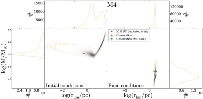
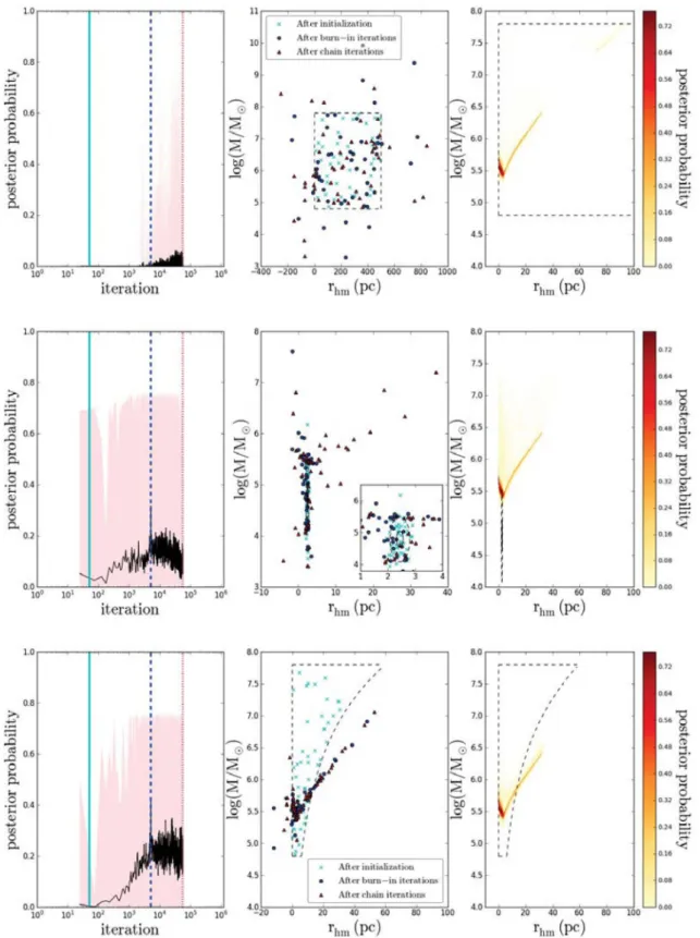
Figure 2. A simple example of the results for the cluster M4. Initial and final condition distributions in half-mass radius versus total mass, where the three panels on the left show the initial conditions and the three panels on the right show the final conditions. The square panels show the two-dimensional histograms in log(M) versus log(rhm) of the 99.7 per cent confidence region of the simulations that fit the observables without a correction for MS in a black–white density plot: the darker the area, the more initial conditions were sampled in this area. Overplotted on these two-dimensional histograms are the outer contours of the two-dimensional histograms of the 99.7 per cent (yellow dotted line) confidence level initial conditions for both the simulations without a correction for MS, with the projected histograms for log(rhm) at the top and for log(M) on the left, respectively, right-hand side. The yellow square with error bars show the observation of the cluster’s current mass and half-mass radius when no correction for MS is made, and the cyan square with error bars shows the observable with a correction. The pink filled circle in the left-hand panel denotes the initial condition used by the DS, which evolves to the final condition shown by the pink filled circle in the right-hand panel.
posterior probabilities; (2) from the set of initial conditions with the highest normalized posterior probability downwards, we sum the normalized posterior probabilities of each subsequent set of initial conditions until this sum equals 0.997 (0.683). The sets of initial conditions included in that sum are a subset of initial conditions that make up 99.7 per cent (68.3 per cent) of the total posterior proba-bility, i.e. the 99.7 per cent (68.3 per cent) confidence region. Note that our definition of the 99.7 per cent confidence region is different from what is usually meant with a 99.7 per cent confidence region, namely the region containing 99.7 per cent of all the data points. The reason for our alternative definition is that our aim is to show those regions of initial conditions with high posterior probability and if we were to use 99.7 per cent of all the data points, this re-gion would contain a large number of initial conditions with low posterior probability (p<0.01).
In Fig.2, we show a simple example of our results for the cluster M4 without a correction for MS, whereby the 99.7 per cent confi-dence region in both the initial and the final conditions are enclosed by the yellow, dotted contours.
3 VA L I DAT I O N
3.1 Validation strategy
We validate our method by applying it to nine star clusters that have been studied to great extent with eitherN-body simulations or Monte Carlo methods. These nine clusters include one Galactic open cluster, seven Galactic globular clusters and one extragalactic globular cluster; see Table 1 for the names of the clusters, the cluster types, their host galaxy, the references to papers in which these clusters were studied and with which simulation technique.
3.1.1 Direct comparison
The first step in the validation is to do a direct comparison of the cluster evolution codes by starting from the same sets of initial conditions and evolving the cluster under conditions which are as similar as possible. Therefore, for each cluster we start at the (best-fitting) set of initial condition put forward by the dedicated studies (DSs) and we evolve this cluster up to the same age under similar conditions, which we describe in Section 3.2 and summarize in Table2.
3.1.2 IndependentEMACSS-MCMCruns
The second step is to run ourEMACSS-MCMCmethod (Section 2.2)
in-dependently and determine which initial masses and half-mass radii reproduce the cluster observables best, explore possible degenera-cies therein and observe whether the best-fitting initial conditions of the DS are contained within our confidence regions. For the sake of comparison to the mentioned DSs, we adopt the cluster observables that were used in the references mentioned in Table1, even though some cluster parameters are presently better constrained by more recent studies, see e.g. table 1 of the recent study of Marks & Kroupa (2010), where present-day masses and half-mass radii are listed for a number of clusters. Our goal in this paper is to validate our method by comparing our results to the results which were obtained with the DSs. Therefore, it is more important to adopt the observables from these studies than to use the currently best constrained observables. See Section 3.2 and Table2.
The next step is to exploit the power of MCMC. In the five-dimensional version of ourEMACSS-MCMCmethod, we add the
Table 1. The nine star clusters on which we apply our method to validate it. The first column lists the name of the cluster, the second column the cluster type and the third column the galaxy in which the cluster resides. The fifth column shows the references to the studies which already studied these clusters to great extent with the simulation technique mentioned in column four. The clusters are mentioned in the order of increasing current half-mass relaxation time that was taken from the Harris Catalogue (Harris2010), except for the first and last mentioned cluster, where we took the relaxation times from the corresponding reference in this table. See Table2for the values of these relaxation times.
Name Cluster type Galaxy Simulation technique Reference M67 Open cluster Milky Way DirectN-body Hurley et al. (2005) NGC 6397 Globular cluster Milky Way Monte Carlo Giersz & Heggie (2009) M4 Globular cluster Milky Way Monte Carlo Heggie & Giersz (2008) M22 Globular cluster Milky Way Monte Carlo Heggie & Giersz (2014) Palomar 4 Globular cluster Milky Way DirectN-body Zonoozi et al. (2014) 47 Tuc Globular cluster Milky Way Monte Carlo Giersz & Heggie (2011) Palomar 14 Globular cluster Milky Way DirectN-body Zonoozi et al. (2011) ωCen Globular cluster Milky Way Monte Carlo Giersz & Heggie (2003) G1 Globular cluster M31 ScaledN-body Baumgardt et al. (2003b)
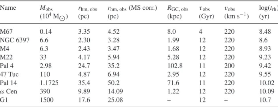
Table 2. Observational data of the validation clusters as used in the references mentioned in Table1. The first column lists the cluster name and the second column the observed mass in 104M
. The third and fourth columns lists the half-mass radius without a correction for MS (i.e. equal to the 3D half-light radius) and the half-mass radius with a correction for MS, respectively. The galactocentric radius, age, orbital velocity of each cluster as used in the references mentioned in Table1are listed in column five, six and seven, respectively. For the sake of comparison to these DSs, we use these observables in our simulations, even though some cluster parameters are presently better constrained by more recent observations. See Section 3.2 for the reasoning behind choosing each of these parameter values. Name Mobs rhm, obs rhm, obs(MS corr.) RGC, obs τobs vobs log(trh)
(104M
) (pc) (pc) (kpc) (Gyr) (km s−1) (yr)
M67 0.14 3.35 4.52 8.0 4 220 8.48
NGC 6397 6.6 2.30 3.28 1.99 12 220 8.6
M4 6.3 2.43 3.47 1.68 12 220 8.93
M22 33 4.17 5.94 5.28 12 220 9.23
Pal 4 2.98 24.7 35.2 102.8 11 200 9.42
47 Tuc 110 4.87 6.94 2.95 12 220 9.55
Pal 14 1.1725 35.4 50.2 71.6 11 220 10.02
ωCen 390 9.89 14.09 1.22 12 220 10.09
G1 1500 17.6 25.08 – 12 – 10.7
and determine the most probable initial masses and half-mass radii. By comparing this to the results of the two-dimensional runs ex-plained above, we can explore how dependent probable initial masses and half-mass radii are on the choice of the galactocentric radius,RGC, age,τ, and velocity,v. Adding these parameters as
nui-sance parameters is observationally motivated, since all observables are always determined with some error. The method here is similar to the description in Section 2.2, but the difference is that now at each iteration we also sample a galactocentric radius, an age and an orbital velocity from Gaussian distributions with the mean equal to RGC, obs,τobsandvobs, respectively, as adopted from the references
mentioned in Table1, see Table2, and a standard deviation equal to 10 per cent of the mean. For G1, though, we takeRGC, obs=40 kpc
as mentioned in Baumgardt et al. (2003b) andvobs=230 km s−1.
We perform our 5D runs only without a correction for MS. The final step is to investigate the stability of our determined ini-tial conditions against errors in the observed data. We do this in two ways. We first compare our 2D. The second thing we do, is checking how increasing/decreasing the error bars on the fitting parameters (log (M) andrhm) will affect the distribution of initial conditions.
The second thing we do, is testing the stability of the initial con-ditions against varying the parametersRGC,vand τ within their
error bars, assuming that the observed mass and half-mass radius are unchanged. We take 10 per cent errors and look at the maximum difference, e.g. comparing a simulation withRGC=RGC, obsto
sim-ulations withRGC=RGC, obs +0.1RGC, obs andRGC=RGC, obs−
0.1RGC, obs, respectively.
3.2 Validation clusters
3.2.1 ωCentauri, M4, NGC 6397, 47 Tucanae and M22
In this section, we describe the studies using the Monte Carlo code
MOCCA(Giersz1998,2001,2006) modelling five Galactic globular
clusters:ωCen (NGC 5139; Giersz & Heggie2003), M4 (NGC 6121; Heggie & Giersz2008), NGC 6397 (Giersz & Heggie2009), 47 Tuc (NGC 104; Giersz & Heggie2011) and M22 (NGC 6656; Heggie & Giersz2014). Hereafter, we refer to these five studies as GH03-14.
the age of the cluster, which was taken to be 12 Gyr for each of these clusters. For M4, NGC 6397, 47 Tuc and M22 their simula-tions included prescripsimula-tions for single and binary stellar evolution, for the Galactic tidal field, for two-body relaxation and for binaries and their dynamical interactions. Forω Cen, which was studied with an early version ofMOCCA, their simulation included simple
prescriptions for single stellar evolution and for the dynamical evo-lution in the Galactic tidal field. After evoevo-lution these clusters gave a satisfactory match to a number of observed characteristics, such as the surface brightness profile and the velocity dispersion profile. See the references mentioned in Section 3.2.1 for the details of their
MOCCAcode.
Orbit and tides.GH03-14 evolved each of these clusters on a cir-cular orbit with a circir-cular velocity of 220 km s−1.5They set the tides
by imposing an initial tidal radius,rt, i. Given this tidal radius and
their initial total cluster mass,M, and assuming an isothermal model for the Galaxy, we calculate per cluster with which Galactocentric radius,RGC, their model is consistent by combining equations (1)
and (2). We use these Galactocentric radii as input for our simula-tions, see the fifth column of Table2.
They evolved their model clusters with an initial tidal radius of 35, 86, 40, 89 and 90 pc, which are consistent with a Galactocentric radius of 1.68, 2.95, 1.99, 5.28 and 1.22 kpc for the clusters M4, 47 Tuc, NGC 6397, M22 (we compare to their model B, see table 1 of Heggie & Giersz2014) andωCen, respectively. Given the fact that M4 is on an eccentric orbit with (eccentricitye, perigalacticon Rp/kpc, apogalacticonRa/kpc) of about (0.8, 0.6, 5.9; Dinescu,
Gi-rard & van Altena1999), this cluster experiences strong tides near perigalacticon. Therefore their choice of the initial tidal radius, and its corresponding galactocentric radius, are very reasonable and bet-ter than evolving the clusbet-ter at its current Galactocentric radius of 5.9 kpc (Harris2010): the averaged tidal field experienced by their cluster during its 12 Gyr circular orbit with a Galactocentric radius of 1.68 kpc is comparable to the tidal field experienced by M4 in its actual eccentric orbit. Their choices for the initial tidal radii for NGC 6397 and M22 with (e,Rp,Ra) of about (0.34, 3.1, 6.3) and
(0.53, 2.9, 9.3), respectively, (Dinescu et al.1999) are also reason-able, but their choices forωCen and 47 Tuc with (e, Rp,Ra) of
about (0.67, 1.2, 6.2) and (0.17, 5.2, 7.3), respectively, are slightly overestimating the effect of the tidal field. However, in order to have a good comparison to the studies mentioned above, for each of these clusters we evolve all our model clusters on a circular orbit with a circular velocity of 220 km s−1at the Galactocentric radius
to which these models are consistent with, see Table2.
Observed mass and radius. GH03-14 get the observational mass of M4 of 6.3 ×10⁴M
from Richer et al. (2004) and got the observed half-light radius from Harris (1996), which in turn lists angular half-mass radii, stated to be taken from the direct average of Trager, King & Djorgovski (1995) and van den Bergh, Morbey & Pazder (1991). Since both latter studies obtain their half-light radii from projected data, we assume that Harris (1996) used a one-to-one relation between half-light radii and half-mass radii, since Harris (2010) lists half-light radii and these values are in many cases very similar to the in Harris (1996) mentioned ‘half-mass radii’. The 2.3 pc for the half-light radius mentioned in table 2 of Heggie & Giersz (2008) is a mistyped value (Heggie, private communication), since the angular projected half-light radiusθphl
given in Harris (1996) is 3.65 arcmin (see also table 1 of Giersz &
5Giersz & Heggie (2003) do not mention which circular velocity they adopted, but we assume it was a value of 220 km s−1as well.
Heggie2009). In combination with the distance between M4 and the Earth,RE=1.72 kpc mentioned in Heggie & Giersz (2008), θphlconverts torphl=1.83 pc using equation (6). We therefore use
rphl=1.83 pc; for the conversion to the 3D half-mass radiusrhm
with a correction for MS (see Section 2.3), we use the relation (8) withcMS=1.9.
GH03-14 got the observational mass for 47 Tuc of 1.1×10⁶M
from Meylan (1989), for NGC 6397 of 6.6×10⁴M
from Drukier (1995) and forωCen of 3.9×10⁶M
from Pryor & Meylan (1993). They do not mention the observational cluster mass of M22, so we take the cluster mass of 3.3×10⁵M
from Richer et al. (2008). GH03-14 got the observed radius for 47 Tuc of 2.79 arcmin and for NGC 6397 of 2.33 arcmin both from Harris (1996); they do not mention the observational radius forωCen and M22, so we get the observed radius forωCen of 5.00 arcmin from Harris (1996) and for M22 of 3.36 arcmin from Harris (2010), respectively. Using the same reasoning as mentioned for M4, we assume the mentioned observed radii to be the projected (2D) angular half-light radiiθphl.
We calculate rphl in by using equation (6) in combination with
distances of 47 Tuc, NGC 6397,ωCen and M22 to the Earth,RE, of
4.5 kpc (Giersz & Heggie2011), 2.55 kpc (Giersz & Heggie2009), 5.1 kpc (Harris1996) and 3.2 kpc (Harris2010), respectively. For the conversion to the 3D half-mass radiusrhmwith a correction for
MS, we use the relation (8) withcMS=1.9.
Model initial and final conditions.The best-fitting sets of initial conditions GH03-14 found for NGC 6397, M4, 47 Tuc and M22 (model B) in (mass/ M, half-mass radius/pc) are listed in Table3. ForωCen Giersz & Heggie (2003) mention the initial and final mass of their best-fitting model (we list those in Table3), but they do not mention the initial and final half-mass radii of that model, only their initial and final tidal radii. Assuming that the tidal radius is the edge radius of the King model initially (Heggie, private communication), we can calculate the initial half-mass radius by using the ratio of tidal-to-half-mass radius taken from fig. 8.3. in Heggie & Hut (2003). Usingrt/rhm∼9.65 for a central potentialW0=7.7, we
findrhm, i=9.33 pc. It is not clear whether this assumption is still
valid after 12 Gyr of evolution, so we cannot calculate their final half-mass radius.
3.2.2 Palomar 14 and Palomar 4
In this section, we describe the first published directN-body simu-lations of the two large and sparse Galactic globular clusters, both residing in the outer halo: Pal 14 (Zonoozi et al.2011) and Pal 4 (Zonoozi et al.2014). They use the collisionalN-body codeNBODY6
(Aarseth 2003) on Graphics Processing Unit (GPU) computers. Hereafter, we refer to these two studies by Z11–14.
Simulation Technique.Z11–14 simulate the evolution of Palomar 14 and Palomar 4 and for Pal 14 they compute 65 models and for Pal 4 a total of 20 models, divided in three categories: 1) clusters with a Kroupa (2001) IMF in the range 0.08<M/M<100 (referred to as theircanonical-NSmodel), (2) clusters with a flattened IMF, (3) clusters with a Kroupa (2001) IMF, but with primordial MS. For Pal 14 they computed one additional model with a Kroupa (2001) IMF, but with primordial binaries. See the references mentioned in Section 3.2.2 for the details of their simulations.
Orbit and tides.For Pal 14, Z11–14 varied the initial half-mass ra-dius and mass and evolved each cluster for 11 Gyr on a circular orbit in a logarithmic potential with a circular velocity of 220 km s−1at
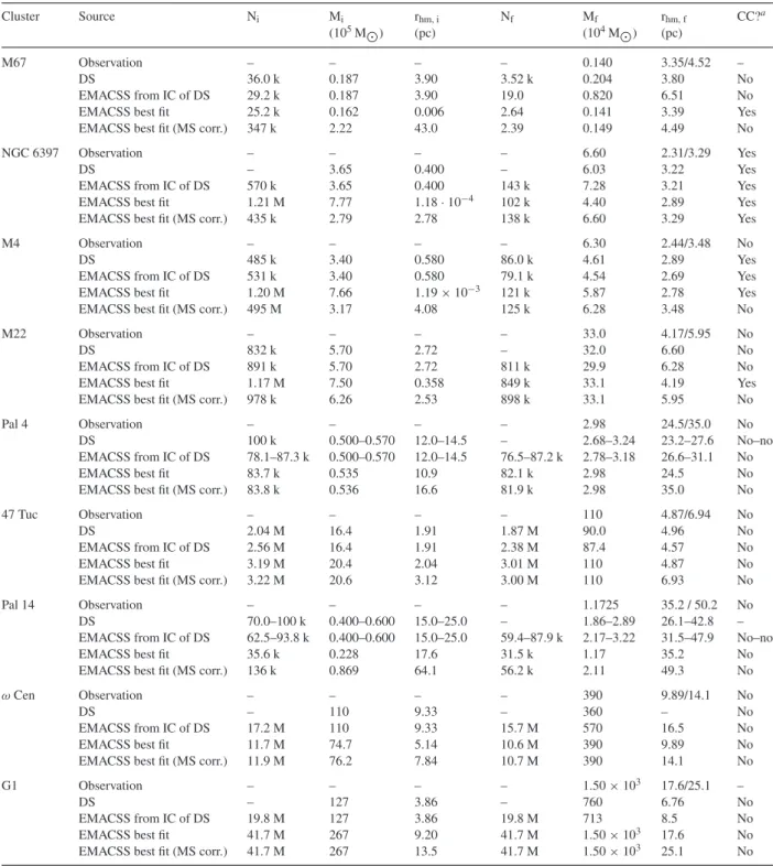
Table 3. Results for the validation in three significant figures. For each validation cluster mentioned in the first column, seven parameters are compared between the observation in the first subrow, the best-fitting results of the DS (see Table1for the references) in the second subrow,EMACSS’ result from the initial condition of the DS in the third subrow,EMACSS-MCMC’ best-fitting results without and with a correction for MS in subrows four and five, respectively (see Section 2.3). The parameters are the initial number of starsNiin column three, the initial mass Mi(in 105M) in column four, the initial half-mass radiusrhm, i(in pc) in column five, the final number of starsNfin column six, the final (current) mass Mf(in 104M) in column seven, the final (current) half-mass radiusrhm, f(in pc) in column eight and the question whether MS has occurred in column nine. The observed value for the current half-mass radius in column eight shows two values: the first one without a correction for MS and the second one with a correction for MS, see Section 2.3 and Table2.
Cluster Source Ni Mi rhm, i Nf Mf rhm, f CC?a
(105M
) (pc) (104M
) (pc)
M67 Observation – – – – 0.140 3.35/4.52 –
DS 36.0 k 0.187 3.90 3.52 k 0.204 3.80 No
EMACSS from IC of DS 29.2 k 0.187 3.90 19.0 0.820 6.51 No
EMACSS best fit 25.2 k 0.162 0.006 2.64 0.141 3.39 Yes
EMACSS best fit (MS corr.) 347 k 2.22 43.0 2.39 0.149 4.49 No
NGC 6397 Observation – – – – 6.60 2.31/3.29 Yes
DS – 3.65 0.400 – 6.03 3.22 Yes
EMACSS from IC of DS 570 k 3.65 0.400 143 k 7.28 3.21 Yes
EMACSS best fit 1.21 M 7.77 1.18·10−4 102 k 4.40 2.89 Yes
EMACSS best fit (MS corr.) 435 k 2.79 2.78 138 k 6.60 3.29 Yes
M4 Observation – – – – 6.30 2.44/3.48 No
DS 485 k 3.40 0.580 86.0 k 4.61 2.89 Yes
EMACSS from IC of DS 531 k 3.40 0.580 79.1 k 4.54 2.69 Yes
EMACSS best fit 1.20 M 7.66 1.19×10⁻³ 121 k 5.87 2.78 Yes
EMACSS best fit (MS corr.) 495 M 3.17 4.08 125 k 6.28 3.48 No
M22 Observation – – – – 33.0 4.17/5.95 No
DS 832 k 5.70 2.72 – 32.0 6.60 No
EMACSS from IC of DS 891 k 5.70 2.72 811 k 29.9 6.28 No
EMACSS best fit 1.17 M 7.50 0.358 849 k 33.1 4.19 Yes
EMACSS best fit (MS corr.) 978 k 6.26 2.53 898 k 33.1 5.95 No
Pal 4 Observation – – – – 2.98 24.5/35.0 No
DS 100 k 0.500–0.570 12.0–14.5 – 2.68–3.24 23.2–27.6 No–no
EMACSS from IC of DS 78.1–87.3 k 0.500–0.570 12.0–14.5 76.5–87.2 k 2.78–3.18 26.6–31.1 No
EMACSS best fit 83.7 k 0.535 10.9 82.1 k 2.98 24.5 No
EMACSS best fit (MS corr.) 83.8 k 0.536 16.6 81.9 k 2.98 35.0 No
47 Tuc Observation – – – – 110 4.87/6.94 No
DS 2.04 M 16.4 1.91 1.87 M 90.0 4.96 No
EMACSS from IC of DS 2.56 M 16.4 1.91 2.38 M 87.4 4.57 No
EMACSS best fit 3.19 M 20.4 2.04 3.01 M 110 4.87 No
EMACSS best fit (MS corr.) 3.22 M 20.6 3.12 3.00 M 110 6.93 No
Pal 14 Observation – – – – 1.1725 35.2 / 50.2 No
DS 70.0–100 k 0.400–0.600 15.0–25.0 – 1.86–2.89 26.1–42.8 –
EMACSS from IC of DS 62.5–93.8 k 0.400–0.600 15.0–25.0 59.4–87.9 k 2.17–3.22 31.5–47.9 No–no
EMACSS best fit 35.6 k 0.228 17.6 31.5 k 1.17 35.2 No
EMACSS best fit (MS corr.) 136 k 0.869 64.1 56.2 k 2.11 49.3 No
ωCen Observation – – – – 390 9.89/14.1 No
DS – 110 9.33 – 360 – No
EMACSS from IC of DS 17.2 M 110 9.33 15.7 M 570 16.5 No
EMACSS best fit 11.7 M 74.7 5.14 10.6 M 390 9.89 No
EMACSS best fit (MS corr.) 11.9 M 76.2 7.84 10.7 M 390 14.1 No
G1 Observation – – – – 1.50×10³ 17.6/25.1 –
DS – 127 3.86 – 760 6.76 No
EMACSS from IC of DS 19.8 M 127 3.86 19.8 M 713 8.5 No
EMACSS best fit 41.7 M 267 9.20 41.7 M 1.50×10³ 17.6 No
EMACSS best fit (MS corr.) 41.7 M 267 13.5 41.7 M 1.50×10³ 25.1 No
aThe results whether a cluster had undergone core-collapse according to observations are taken from Trager et al. (1995), except for G1, where we adopt what Baumgardt et al. (2003b) argued about the core-collapse state of these two clusters.
evolution, they fit the final values for the number of bright stars, the projected half-light radius and the slope of the mass function in the mass range 0.525–0.795 Mto the observed ones. To make a fair comparison, we also evolve all of our model clusters for Pal 14 on a circular orbit at its current Galactocentric radius, for which we adopt a value of 71.6 kpc from Harris (2010) with a circular velocity of 220 km s−1. To the best of our knowledge, there are
no references reporting on the orbit of Pal 14. Jordi et al. (2009) mention that the orbit could possibly be eccentric, in which case evolving the cluster on a circular orbit at the current Galactocentric radius is an underestimation of the tidal field.
For Pal 4, Z11–14 also varied the initial half-mass radius and mass and evolve each cluster for 11 Gyr on a circular orbit with a circular velocity of 200 km s−1at Palomar 4’s current Galactocentric radius
of 102.8 kpc in an analytic Galactic background potential consisting of a bulge, a disc and a logarithmic halo, which they adjusted to resemble the Milky Way.
Observed mass and radius.Z11–14 got the observed total mass for Pal 14 of about 12000 M from Jordi et al. (2009) and for Pal 4 of about 29 800 Mfrom Frank et al. (2012). For Pal 14, Z11–14 got the observed projected angular half-light radiusθphm
of 1.28 arcmin from Hilker (2006), which they in turn convert to the projected (2D) half-light radiusrphlof 26.4±0.5 pc and a 3D
half-light radius rhl of 35.4±0.6 pc. For Pal 4, Z11–14 got the
observed projected angular half-light radiusθphm of 0.62 arcmin
from King (1966) model fitting on Wide Field Planetary Camera 2 (WFPC2) data and broad-band imaging with the Low-Resolution Imaging Spectrometer at the Keck II telescope, which they convert to the projected (2D) half-light radiusrphlof 18.4±1.1 pc and a 3D
half-light radiusrhlof about 24 pc. We converted these projected
half-light radii to the 3D half-mass radiirhmwith a correction for
MS (see Section 2.3) by using the relation (8) withcMS=1.9.
Model initial and final conditions.For both Pal 14 and Pal 4, we compare to their canonical-NS models, since these models are most comparable toEMACSS. For Pal 14, these are the 28 models
mentioned in table 1 of Zonoozi et al. (2011) with initial masses in the range 40 000–60 000 M(Zonoozi, private communication) and initial half-mass radii in the range 15–25 pc. For Pal 4, these are the seven models mentioned in table 1 of Zonoozi et al. (2014) with initial masses in the range 50 000–57 000 Mand initial half-mass radii in the range 12–14.5 pc (Zonoozi, private communication). The fact that these are not their best-fitting models is not a problem for validation purposes. However, in our Figs10and12, showing the results of the independentEMACSS-MCMCruns in 2D, we also plot
all the other models of Zonoozi et al. (2011,2014) to see if their other (including best-fitting) models are contained in our confidence regions.
3.2.3 G1
In this section, we describe the study using scaledN-body modelling to investigate the evolution of M31’s largest globular clusters G1 (Mayall II; Baumgardt et al.2003b). They use the collisionalN-body codeNBODY4 (Aarseth1999) on the GRAPE-6 computers (Makino
et al.2003).
Simulation Technique.Baumgardt et al.2003bsimulate the evo-lution of G1 by running simulations for star clusters withN=65 536 stars, since directN-body simulations with a number of stars similar to the number of stars present in G1 (N∼107according to
Baum-gardt et al.2003b) was, and still is, out of reach. They used the same half-mass relaxation timetrhfor their model as was inferred for G1
from observations (Meylan et al. 2001estimatedtrh ∼ 50 Gyr).
They perform several dozen of runs to determine their best fit to the surface density, velocity dispersion, rotation and ellipticity profiles. Baumgardt et al. (2003b) constructed two models: (1) a single non-rotating cluster, and (2) a non-rotating merger product, where the merger occurred during the formation process. They varied the initial den-sity profiles, half-mass radii, total masses, and global mass-to-light ratios M/L and evolve each cluster for 13 Gyr. The authors construct the final density and velocity profiles from 10 snapshots in the range 11.75–12.25 Gyr and give their final cluster mass and half-mass ra-dius at 12 Gyr. They use a Kroupa (2001) mass function in the range 0.1< M/M< 30 and include the effects of stellar evo-lution and two-body relaxation. Their simulations do not contain primordial binaries, as G1 should still be far from core-collapse. See the reference mentioned in Section 3.2.3 for the details of their simulation.
Orbit and tides.Baumgardt et al. (2003b) do not include a tidal field, since they argue that the tides would have a negligible effect on the cluster’s evolution, since the cluster is currently at a distance of 40 kpc to the centre of M31 (Meylan et al.2001). We therefore evolve all our model clusters for G1 for 12 Gyr without including a tidal field (i.e. as an isolated cluster); see Table2.
Observed mass and radius.Baumgardt et al. (2003b) got a set of observed half-mass radii rhm in the range 12.3–15.0 pc and
observed total masses in the range 7.3–17×106M
from Mey-lan et al. (2001), who in turn estimated the half-mass radii and masses from the surface brightness profile from Hubble Space Telescope/WFPC2 images and velocity dispersion profile from KECK/HIRES (High Resolution Echelle Spectrometer) spectra in combination with King model, King–Michie model and virial the-orem estimates. We choose to compare our results to the observ-ables which they obtain with their King–Michie model nr 4, which gives somewhat average values of the above mentioned ranges: rhm =13.2 pc, M =15 ×106Mand trh∼ 50 Gyr. However,
we have checked that the ‘half-mass radius’ mentioned in Meylan et al. (2001) comes from their angular projected radii in arcmin by using equation (6) in combination with its distance to the Earth RE=770 kpc, which they provided in their Table1. They do not
mention that they corrected for projection (factor 4/3) or that they did any correction for MS. We therefore assume that the radius they refer to as the half-mass radius is actually the projected half-light radius. For the conversion to the 3D half-mass radiusrhmwith a
correction for MS (see Section 2.3), we use the relation (8) with cMS=1.9.
Model initial and final conditions.For G1, we compare to their non-rotating model, since this model is most comparable toEMACSS.
After scaling up, the cluster of this model obtained a final mass of 7.6×10⁶M
and a final half-mass radius of 6.76 pc (Baum-gardt et al.2003b). They found that during the evolution the cluster mainly expanded by a factor of 1.75 due to stellar evolution and that it lost about 40 per cent of its mass over 12 Gyr (Baumgardt, private communication). From this, we calculated an initial mass of 1.27×10⁷M
and an initial half-mass radius of 3.86 pc.
3.2.4 M67
In this section, we describe the work using directN-body modelling to study the evolution of the rich and relatively old Galactic open cluster M67 (NGC 2682; Hurley et al.2005). The authors simulate the evolution of M67 by using the collisionalN-body codeNBODY4
Simulation Technique.Hurley et al. (2005) modelled the evolu-tion of M67 by performingN-body simulations. They compared their modelled surface density profile to the surface density profile of M67 of Bonatto & Bica (2005) provided by Bonatto (private com-munication), their modelled colour–magnitude diagram (CMD) to the observed CMD of Montgomery, Marschall & Janes (1993) and their modelled luminosity function and their structural parameters such as the half-mass radius to the observational data from Fan et al. (1996). They furthermore extensively study the stellar pop-ulations in their simulation and especially focus on the formation channels of blue stragglers (BSs) and compare their results to ob-servational data from Fan et al. (1996), Latham & Milone (1996), Milone & Latham (1992) and Leonard (1996). For the single stars, they use a Kroupa, Tout & Gilmore (1993) mass function in the range 0.1<M/M<50 and their model fully accounts for the effects of cluster dynamics as well as stellar and binary evolution, including a significant fraction of primordial binaries. Hurley et al. (2005) constructed two different models, differing only in the initial mass, the Galactocentric radius and the binary period distribution. Their second and favoured colour model are ran for a star cluster withN=36 000 stars. See Hurley et al. (2005) for the details of their models and theN-body code they used.
Orbit and tides.We compare to the second model of Hurley et al. (2005), because it is their best-fitting model. In this model, they evolved the cluster for 4 Gyr on a circular orbit with a circular velocity of 220 km s−1at a Galactocentric radius of 8.0 kpc, which
is a reasonable choice for a cluster on an slightly eccentric orbit with a perigalaciticon of 6.8 kpc and a apogalacticon of 9.1 kpc (Carraro & Chiosi1994).
Observed mass and radius. The half-mass radius of main-sequence stars observed within 10 pc that Hurley et al. (2005) used was taken from Fan et al. (1996), who determined it to be 2.5 pc. However, we checked that the ‘half-mass radius’ mentioned in Fan et al. (1996) comes from converting their angular projected radii in arcmin by using equation (6) in combination with the cluster’s distance to the Earth,RE=783 pc, calculated from their provided
distance modulus of 9.47 mag. They do not mention that they cor-rected for projection (factor 4/3) or that they did any correction for MS. We therefore assume that the radius they refer to as the half-mass radius, is actually the projected half-light radius. For the conversion to the 3D half-mass radiusrhmwith a correction for MS
(see Section 2.3), we use the relation (8) withcMS = 1.8. Both
studies took the total luminous cluster mass from Fan et al. (1996), which determined that to be 1000 M. Hurley et al. (2005) esti-mated that this luminous mass represented a total cluster mass of about 1400 M.
Model initial and final conditions.The best-fitting initial condi-tions Hurley et al. (2005) found for M67 (model 2) in (mass/ M, half-mass radius/pc) are listed in Table3.
4 R E S U LT S
4.1 Performance
In this section, we test the performance of theEMACSS-MCMCmethod.
We first determined a suitable number of the walkers,nw, burn-in
iterations,nb, and subsequent chain iterations,nc, such that we have
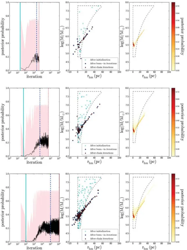
a good balance between proper coverage and quick convergence. To this end, we ran a dozen simulations for the cluster M4 varying these three numbers and plotting the posterior probability of an iteration as a function of the iteration number. We divided all the iteration in bins of 50 iterations and calculated the minimum, maximum and
mean probability per bin, see Fig.3. In these simulations, we used a prior distribution that is uniform in mass (similar to the first line of equation 3), but semi-uniform in half-mass radius: the upper limit of the half-mass radius is mass-dependent through the dependence on the Jacobi radius,rJ:
log(Mobs)≤log
M M
≤log(Mobs)+3,
0< rhm
pc <0.3rJ. (9)
This mass-dependent upper limit of the initial half-mass radius is motivated by the fact that most clusters with initial half-mass radii larger than 30 per cent of the Jacobi radius will quickly dis-solve (Alexander et al.2014). As we show later on in this section, initializing the walkers according to this prior does not exclude the parameter space withrhm/rJ>0.3, but it does accelerate the
convergence.
In order to judge whether the walkers have converged, we look at the instance that both the maximum and the mean posterior probability have stabilized, which means that its value does not increase or decrease by a significant amount, say 100 per cent, and thus only show the variation caused by the scatter. The scatter in the mean posterior probability is a natural feature of any MCMC sampler, because it is important that even though a (local) maximum in posterior probability has been found, the walkers continue to explore other regions of parameter space, in order to locate possible other maxima.
From the first row of Fig.3, showing the simulation with (nw,
nb,nc)=(20, 100, 100), we see that the walkers already start to
converge after about 2000 iterations, marking the end of the burn-in phase. However, from the right-hand column of the first row, we see that the coverage of theM–rhmplane is still poor, meaning that we
can observe by eye that the two-dimensional parameter space is not well-sampled and/or that the sampled region does not cover a large region of that parameter space. In the second row of Fig.3, we see that both convergence and proper coverage, by eye, seem to have been established for the simulation with (nw,nb,nc)=(50, 100,
1000): the walkers probed a wide range of initial masses and half-mass radii in proposing initial conditions. Nevertheless, we have chosen to be conservative and to use (nw,nb,nc)=(50, 100, 1000)
only fortest simulations6 and to use (n
w, nb,nc) =(100, 1000,
10000) for all main simulations in this work, see the third row of Fig.3.
We secondly determined whether the choice of a prior distribution would affect the ranges of parameter space that are covered and thus the determined probable initial condition distribution. To test this, we ran three simulations to determine the initial conditions for the cluster M4 with (nw,nb,nc)=(50, 100, 1000) using three different
priors, but otherwise being the same. These three priors were
(1) a uniform distribution in both (logaritmic) mass and half-mass radius, according to equation (3);
(2) a normal distribution in both parameters with the mean equal to log (Mobs) andrhm, obs, respectively, and a standard deviation equal
to 10 per cent of the mean;
(3) a semi-uniform distribution, according to equation (9).
The results of these three simulations are shown in Fig.4. From this figure, we can see that the covered area in theM–rhm plane
of the probable initial conditions is similar. If we consider all sampled initial conditions (also those outside of the boundaries given by equation 3, e.g. negative half-mass radii, with poste-rior probabilities equal to zero, which is not shown in Fig. 4), the sampled area is significantly different: the simulation with a uniform prior covers a larger range in initial half-mass radius (−500(rhm,i/pc)1000) and slightly different, but overlapping
range in logarithmic mass (2.0log(Mi/M)10.5) compared
to the semi-uniform prior (−68.9 (rhm,i/pc)150 and 2.9
log(Mi/M)9.8) and the normal prior(−26.9 (rhm,i/pc)
60.4 and 1.1log(Mi/M)9.1). If we consider initial
condi-tions with posterior probability greater than zero, then the covered area is slightly more similar: the walkers initialized according to a uniform prior reach larger initial half-mass radii, but the initial mass range is comparable (uniform: 10−3<(r
hm, i/pc)<95.7 and
5.3<log (Mi/M)<7.8; semi-uniform: 10−4<(rhm, i/pc)<63.8
and 5.3<log (Mi/M)<7.8; normal: 10−4<(rhm, i/pc)<58.0
and 5.3 <log (Mi/M) <7.7). We observe in the top panel of
Fig. 4that there is an area of initial conditions with high initial mass and high initial radius, that is not probed with the simulations with the other two priors. However, this is not a favourable region in terms of posterior probability and thus we conclude that simulations with different prior distributions properly cover the relevant ranges of parameter space and that the derived initial conditions are prior independent. Similar behaviour is seen for the other clusters in our sample. We use the semi-uniform prior distribution for the rest of our simulations in this work.
The final performance characteristic to test is the sampling of initial conditions by the walkers. The results of all the simulations for both the 2D and 5D runs are shown in Figs6–14, Fig.15and FigsA1–A8. By comparing the two-dimensional histograms with the confidence contours in these figures, we see that the most sam-pled areas overlap with the high posterior probability regions. This is what one would expect for an MCMC method with a sufficient number of iterations, and hence shows the proper performance of our method. We note that the number of sets of initial conditions in the 99.7 and 68.3 per cent confidence regions is less than∼99.7 per cent, respectively,∼68.3 per cent, of the total number of surviving initial conditions, and that increasing the number of iterations does not increase these percentages. For instance, for M4 the number of sets of initial conditions in the 99.7 and 68.3 per cent confidence regions is∼80 per cent, respectively,∼40 per cent of the total number of surviving initial conditions for both the simulation with (nw, nb,
nc)=(50, 100, 1000) and the simulation with (nw,nb,nc)=(100,
1000, 10000). This is again because even though the walkers have converged to high posterior probability regions of parameter space, they continue to sample unexplored regions as well.
4.2 Direct comparison
Fig.5shows the direct comparison betweenEMACSSand the DSs by
runningEMACSSfrom their best-fitting initial condition. All results
presented in this section are summarized in Table 3, where we compare the best-fitting results of the DS andEMACSS’ result when
starting from the initial condition of the DS in row two and three for each cluster.
From Fig.5, we see that theEMACSSresults compare quite well to
the Monte Carlo and theN-body results for NGC 6397, M4, M22, Pal 4, 47 Tuc, Pal 14 and G1, with a difference in final conditions <25 per cent with respect to the DSs in both (linear) mass and half-mass radius for each of these clusters. For M4, M22 and 47 Tuc, we see that the evolution withEMACSSled to a close match
in final conditions (with<8 per cent difference in both mass and half-mass radius) losing slightly more mass during its evolution, and reaching smaller final radii. For these three clusters the final radii are smaller, because the cluster did not expand as much as in theMOCCAsimulation. For M4, the radius did expand up to 2.87 pc
in the evolution withEMACSS, but near the end of the simulation the
cluster already started to contract due to stellar evaporation. For NGC 6397, we have almost an exact match in final half-mass radius (<1 per cent difference), but the amount of mass-loss is less, leading to a difference of∼21 per cent in linear mass with respect to the DS.
For G1, the cluster modelled withEMACSS more mass than the
cluster modelled with a scaledN-body simulation (∼6 per cent dif-ference in mass), but it also expanded more (∼25 per cent differ-ence in radius). However, we note that in calculating the scaled-up version of the initial mass and half-mass radius of G1 found by Baumgardt et al. (2003b), we assumed that the same amount of mass-loss and stellar evolution induced expansion occurred as in the small-scale model. This does not have to be the case. Therefore, it could be that the scaled up initial condition from which we start evolving withEMACSSis different from the actual scaled up version
of the initial condition of Baumgardt et al. (2003b), which would cause the differences in final mass and half-mass radius. For Pal 4 and Pal 14, we see that on average the directN-body modelling caused the modelled clusters to lose slightly more mass than the clusters modelled withEMACSSleading to<15 per cent difference
in mass for Pal 4 and<21 per cent difference in mass for Pal 14. For both Pal 14 and Pal 4, theEMACSSclusters expanded a bit more
(<4 per cent and<2 per cent difference in radius, respectively). For ωCen, theEMACSS results compare less well to those
ob-tained fromMOCCA. Their simulated cluster lost substantially more mass (leading to an∼59 per cent difference in linear mass). We could not compare the final half-mass radii, since Giersz & Heggie (2003) did not provide this, as described in Section 3.2.1. It could be that our assumption for calculating what the initial half-mass radius for the best fit of Giersz & Heggie (2003, see Section 3.2.1) was incorrect and that their initial half-mass radius was somewhat smaller or larger. Starting at a different initial radius could lead to a different amount of mass-loss. However, we have done sev-eralEMACSSruns forωCen, starting at the same initial mass, but with different initial half-mass radii in the range 0.01–30 pc and we saw that the amount of mass-loss changed only minimally. The mass-loss changed at most by a factor∼1.08 between two radii in this range. For initial half-mass radii>20 pc the amount of mass-loss decreased. Only for clusters initially more compact than 0.5 pc will the amount mass-loss increase significantly, but not as much as in theMOCCAsimulation. It is also not likely thatωCen started out so compact, see Section 4.3. There is also poor agreement be-tweenEMACSS and the directN-body results for the open cluster M67. Again, we see that the cluster simulated withEMACSSlost
sub-stantially less mass. Furthermore, theEMACSScluster expanded by
almost a factor 2 during its evolution, whereas the final half-mass radius of the cluster modelled with directN-body integration is even slightly smaller than the initial one. These differences require some explanation.
Besides starting from the same initial total mass and half-mass radius, we kept the conditions of our simulation as similar as possi-ble to those of the DSs. However, there are a number of parameters that could not be taken equal between the codes. One of these pa-rameters is the initial number of stars. SinceEMACSSis currently