The handle http://hdl.handle.net/1887/97593 holds various files of this Leiden University dissertation.
Author: Raasveldt, M.
Proefschrift
ter verkrijging van
de graad van Doctor aan de Universiteit Leiden,
op gezag van Rector Magnificus prof.mr. C.J.J.M. Stolker,
volgens besluit van het College voor Promoties
te verdedigen op dinsdag 9 juni 2020
klokke 11:15 uur
door
Mark Raasveldt
geboren te Leiderdorp
Promoter: prof. dr. Stefan Manegold (CWI & Leiden University) Co-promoter: dr. Hannes M¨uhleisen (CWI)
Overige leden: prof. dr. Aske Plaat (Leiden University) prof. dr. Thomas B¨ack (Leiden University) dr. Mitra Baratchi (Leiden University) prof. dr. Jens Dittrich (Saarland University) prof. dr. Torsten Grust (University of T¨ubingen)
The research reported in this thesis has been carried out at the CWI, the Dutch
National Research Laboratory for Mathematics and Computer Science, within the
Database Architectures group.
The research reported in this thesis has been carried out under SIKS, the Dutch
Research School for Information and Knowledge Systems.
This research is financially supported by the Dutch funding agency NWO, under project
number 650.002.001 (the PROMIMOOC project), in collaboration with Tata Steel
Ijmuiden, BMW Group Regensburg, Leiden University and Centrum voor Wiskunde
When I was studying for my masters in university I always thought that I would
never do a PhD. After all, you get paid less than working in industry and you need
to work on theoretical research instead of solving practical problems. The reason
that I opted to do a PhD anyway is because of Hannes, Stefan and the rest of the
Database Architectures group. They showed me that not only can research be useful
and practical, it can be amazingly fun and engaging as well. I have learned so much
in my time here and am very thankful to each of the members of the DA group that
have provided me with their knowledge and wisdom.
I am particularly indebted to Hannes, who took me in as a master student and has
worked closely with me ever since. All of the days that we spent peer programming
were extremely fun and informative. I would also like to give special thanks to my
promotor Stefan. Firstly for giving me the opportunity of doing my PhD at the
CWI, and secondly for being extremely kind and compassionate and creating such
an accepting and amazing workplace. They say that how you experience your PhD
depends entirely on your supervisor, and I had the best supervisors that I could wish
for in Hannes and Stefan.
In my time at the CWI I have made many friends that have made my time there
extremely pleasant. Pedro, Tim and Diego who I could always count on to have a
good time and with whom I share many amazing memories. Thibault, who has taught
me how to enjoy the pleasantries of life and how to write introductions. Abe, who has
always impressed me with his math skills. Till, who was always ready to beat me in a
game of table tennis. And finally, I would like to thank all the other people of the DA
group for making my time there so special and amazing.
Finally, I would like to acknowledge my family and friends for their support. My
mother and father - both also computer scientists - who have always supported me in
doing whatever I wanted to do, even though I ended up following in their footsteps
anyway. I would also like to thank my siblings, Maarten and Marieke. My close friends
1 Introduction 11
1 The Rise of Data Science . . . 11
2 Tools of the Trade . . . 12
3 Data Science & Data Management . . . 13
4 Our Contributions . . . 14
5 Structure and Covered Publications . . . 15
2 Background 17 1 Relational Database Management Systems . . . 18
2 RDBMS Design . . . 19
2.1 Workload Types . . . 19
2.2 System Types . . . 20
2.3 Physical Database Storage . . . 20
2.4 Database Processing Models . . . 21
3 Database Connectivity . . . 23
3.1 Client-Server Connection . . . 23
3.2 In-Database Processing . . . 24
5 Python . . . 28
3 Database Client-Server Protocols 31 1 Introduction . . . 31
1.1 Contributions . . . 32
1.2 Outline . . . 33
2 State of the Art . . . 33
2.1 Overview . . . 34
2.2 Network Impact . . . 37
2.3 Result Set Serialization . . . 39
3 Protocol Design Space . . . 43
3.1 Protocol Design Choices . . . 44
4 Implementation & Results . . . 54
4.1 MonetDB Implementation . . . 54
4.2 PostgreSQL Implementation . . . 55
4.3 Evaluation . . . 57
5 Summary . . . 62
4 Vectorized UDFs in Column-Stores 63 1 Introduction . . . 63
1.1 Contributions . . . 64
1.2 Outline . . . 65
2 Types of User-Defined Functions . . . 65
3 MonetDB/Python . . . 66
3.1 Usage . . . 66
3.2 Processing Pipeline . . . 67
3.3 Parallel Processing . . . 70
3.4 Loopback Queries . . . 75
4 Evaluation . . . 75
5 Related Work . . . 79
5.1 Research . . . 79
5.2 Systems . . . 82
6 Applicability To Other Systems . . . 83
7 Development Workflow: devUDF . . . 85
7.1 The devUDF Plugin . . . 87
7.2 Usage . . . 87
7.3 Implementation . . . 89
8 Summary . . . 90
5 In-Database Workflows 93 1 Introduction . . . 93
1.1 Contributions . . . 94
1.2 Outline . . . 94
2 Related Work . . . 94
2.1 Machine Learning Integration . . . 94
2.2 Machine Learning Model Management . . . 95
3 Machine Learning integration . . . 96
3.1 Training . . . 97
3.2 Classification . . . 98
3.3 Ensemble Learning . . . 99
4 Experimental Analysis . . . 99
5 Summary . . . 102
6 MonetDBLite 103 1 Introduction . . . 103
1.1 Contributions . . . 104
1.2 Outline . . . 104
2 Design & Implementation . . . 104
2.3 Native Language Interface . . . 107
2.4 Technical Challenges . . . 111
3 Evaluation . . . 113
3.1 Setup . . . 113
3.2 TPC-H Benchmark . . . 114
3.3 ACS Benchmark . . . 121
4 Summary . . . 123
7 DuckDB: an Embeddable Analytical Database 125 1 Introduction . . . 125
1.1 Contributions . . . 127
2 Design and Implementation . . . 128
3 Summary . . . 130
8 Conclusion 133 1 Big Picture . . . 133
2 Future Research . . . 134
2.1 Client-Server Connections . . . 134
2.2 In-Database Processing . . . 135
2.3 Embedded Databases . . . 138
Bibliography 140
Summary 151
Samenvatting 153
Introduction
1
The Rise of Data Science
Analyzing data in order to uncover conclusions, often referred to as “data science”,
is everywhere in todays world. In order to gain value from their data, nearly every
large business has a data science branch or a team of data scientists looking to extract
value from their data. But data analysis is not used only in the financial sector. It
is also widely used in journalism, to aid the decision of government policies, in all
branches of science and in many more areas.
0.0001 0.01 1 100 10000
1960 1970 1980 1990 2000 2010 2019
Year
Price ($/MB)
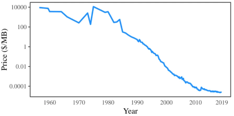
These developments are happening largely because of how cheap gathering, storing
and analyzing large quantities of data have become. When we look back just sixty
years, the IBM 350 disk storage unit was released. The IBM 350 could hold up to
3.75MB of data, and cost approximately 35000USD at the time. Today, we can buy a
HDD with 1TB of storage for around 50USD. To put that into perspective, in 1960
the price of a Chevrolet Impala was around 3000USD. If the price of cars had fallen
at the same rate as the price of hard disks, the newest model of Chevrolet would cost
a mere $4.25 and could drive 200,000 times faster.
Not only has the cost of storing the data become so much cheaper, so has the cost
of reading and processing that data. CPU processing speeds have improved orders of
magnitude following Moore’s Law, and RAM sizes have blown up. The phone in your
pocket has over 10 times more high-speed RAM than the Cray-1 supercomputer had
storage, and has significantly more processing power as well.
Looking at these numbers, it is no wonder that data science has become so
ubiquitous. Analyzing large amounts of data has become very cheap and accessible
even to small companies and individuals. Expensive supercomputers are no longer
needed to store and analyze large amounts of data. Data science can be performed on
cheap commodity hardware. Analyzing 10GB of data on a laptop is common place,
and it is not unheard of to process 100GB or even 1TB of data on a desktop computer.
2
Tools of the Trade
While data science might appear like a brand new field, it is closer to a mixture
of different fields. In particular, it is a combination of mathematics, statistics and
computer science. Many of the techniques applied by data scientists are in fact
techniques from the statistics field that can now cheaply be applied to large quantities
of data because of technological advances.
Many of the tools that are used in data science have actually been designed
and created by statisticians. An example of this is the R project for statistical
S language, a statistical language designed by John Chambers at Bell Labs. R was
originally implemented by the statisticians Ross Ihaka and Robert Gentleman at
Auckland for the purpose of teaching introductory statistics courses. It has grown
into a tool that is used worldwide to perform statistical analysis, data classification
and data visualization.
Another popular language for data science is Python, together with the support
of the numeric python extensions NumPy [84], SciPy [48] and Pandas [64]. While
Python itself does not have its roots in statistics, the numeric python extensions are
based primarily on the APL family of languages, which includes S (the precursor of
R), Fortran and MATLAB. These languages have all been designed primarily for use
in numeric computing and statistics.
3
Data Science & Data Management
One of the consequences of the origins of these tools is that proper data management
was never a first class citizen. Data management is largely treated as an afterthought
in these tools. Typically, the data that is used for analyses is loaded from a data
source into structures residing in memory and then kept around in memory. The tools
do not support larger than memory data sets. Any management of that data is not
handled by the tools themselves, and is left up to the user.
Data scientists typically opt to store the data in a set of flat files, as this is the
most natural way of interacting with these tools. While flat file storage is simple when
dealing with very small data sets that fit in individual files, it does not scale well. Flat
file storage requires tremendous manual effort to maintain when the data sets grow in
size. The files are also difficult to reason about because of the lack of a rigid schema,
and it is difficult to share the data between multiple users. Furthermore, adding new
data or modifying existing data is prone to corruption because of lack of transactional
guarantees and atomic write actions provided by these tools.
All of the problems of flat file storage are not new problems. In fact, database
database management systems prevent data corruption through strong transactional
guarantees and ACID properties, automatically manage data storage and make
data easier to reason about by enforcing a rigid schema. In addition, the database
management systems can perform efficient execution on larger-than-memory data,
and allow safe concurrent access to the data.
However, despite the existence of database management systems, data scientists
typically opt not to use them in conjunction with these analytical tools. This leads us
to our main research problem:
Research Problem How can we facilitate efficient and painless integration of analytical tools and relational database management systems?
4
Our Contributions
In this thesis we work to answer the main research problem by investigating the different
methods of combining relational database management systems and analytical tools.
We consider the three separate methods of connecting analytical tools with RDBMSs:
(1) client-server connections, (2) in-database processing and (3) embedded databases.
For each of these methods, we examine the current state of the art and attempt to
improve on it in both run-time efficiency and usability.
• Client-Server Connections (Chapter 3). We examine the client-server protocols of popular RDBMSs, and evaluate their effciency in the context of
large-scale result export that is required to perform data analysis and machine
learning on large data sets contained within these systems. Based on this
analysis, we propose a new client-server protocol that handles these situations
more efficiently and show its efficiency by implementing it in two open source
RDBMSs.
• In-Database Processing (Chapters 4 and 5). We examine current methods of in-database processing in popular RDBMSs and improve on these methods
in-database analytics: Vectorized UDFs. We implement these in MonetDB, a
popular open-source RDBMS, and show how these UDFs can be effectively used
to perform analytical workflows entirely within the RDBMS.
• Embedded Database: MonetDBLite (Chapter 6). We adopt the popular open-source RDBMS MonetDB to run as an embedded database inside analytical
tools. We show how an embedded database can greatly increase usability of a
database system, as well as show how the speed at which the analytical tool and
the RDBMS can exchange data is greatly improved by embedding the database.
• Embedded Database: DuckDB (Chapter 7). Learning from our imple-mentation of MonetDBlite, we identified the requirements and challenges of an
embedded database system, and created our own RDBMS designed for being
embedded from scratch: DuckDB. DuckDB fixes many of the deficiencies of
MonetDBLite that were caused by the system being initially designed as a
stand-alone server process.
5
Structure and Covered Publications
We present the background material necessary to understand this thesis in Chapter 2.
We discuss the history of relational database management systems, and how they
relate to the field of analytics, and we discuss the various ways in which database
systems can be combined with stand-alone analytical tools.
In the subsequent chapters, we discuss the methods in which we aim to improve over
the existing work. In Chapter 3, we describe our work on improving the client-server
protocol, based on the following paper:
• Don’t Hold My Data Hostage - A Case For Client Protocol Redesign
Mark Raasveldt, Hannes M¨uhleisen
43rd International Conference on Very Large Data Bases (VLDB 2017)
In Chapter 4 we discuss our work on extending user-defined functions for analytical
• Vectorized UDFs in Column-Stores
Mark Raasveldt, Hannes M¨uhleisen
28th International Conference on Scientific and Statistical Database Management
(SSDBM 2016)
In Chapter 5 we discuss our work on embedding analytical workflows inside a
database system. This chapter is based on the following paper:
• Deep Integration of Machine Learning Into Column Stores
Mark Raasveldt, Pedro Holanda, Hannes M¨uhleisen and Stefan Manegold
21st International Conference on Extending Database Technology (EDBT 2018)
In Chapter 6 we discuss our work on extending the MonetDB system into an
em-bedded database system called MonetDBLite. This chapter is based on the (currently
unpublished) paper:
• MonetDBLite: An Embedded Analytical Database
Mark Raasveldt and Hannes M¨uhleisen
In Chapter 7 we discuss our work on creating the embedded database system
DuckDB. This chapter is based on the following paper:
• DuckDB: an Embeddable Analytical Database
Mark Raasveldt and Hannes M¨uhleisen
ACM International Conference on Management of Data (SIGMOD 2019)
Background
As our goal is to improve the coupling of relational database management systems
and analytical tools, it is clear that the existing techniques for combining external
programs and RDBMS servers must be investigated.
In this chapter, we will describe existing techniques for combining external programs
and RDBMS servers, and also provide the necessary background for understanding
these techniques. In Section 1, we give a brief description of the history of RDBMS
engines. In Section 2 we briefly describe the different types of RDBMS engines and
the different physical storage models and database processing models they utilize. In
Section 3 we discuss the different methods in which an external analytical program
work in combination with a RDBMS. In Section 4 we describe the internal design
of MonetDB, a popular open-source RDBMS that we have used as a test-bed for
implementing a lot of the work in this thesis. In Section 5, we briefly describe the
internal design of the CPython interpreter and the NumPy library, as we rely on these
1
Relational Database Management Systems
Database management systems have been around in some form or another for almost
as long as computers themselves have been around. They solve the fundamental
problem of manipulating and persistently storing data for future usage. This is a
problem that is encountered by almost any application. Whether it be a bank manager,
an online store or even a video game, they all require a method of persistently storing
state, updating that state and reading back that state.
The most popular form of database management systems are relational database
management systems. These types of systems allow users to interact with the data
they store using languages based on relational algebra, pioneered by E.F. Codd [16] in
1970. In the relational model, data is organized in n−ary relations where every row
in the relation consists of n different values. Data stored in this model can be stored
into multiple relations, and combined at query time using the join operator (1).
The relational model offers two crucial advantages: (1) data can be stored in a
normalized way, avoiding data duplication and improving data integrity, and (2) the
way data is accessed is separated entirely from the physical way in which the data is
organized, allowing for the engineers that create the database management system
to have complete freedom in the way the data is represented on disk and the way in
which it is accessed. This has allowed relational algebra to stay relevant even while
storage methods, indexing algorithms and query execution models have changed.
After Codd’s paper several languages popped up that were based on relational
algebra. The clear winner, and the language used almost universally by relational
database management systems today, is SQL [12] (Structured Query Language). SQL
was initially developed in 1973 at IBM for use in System R [6] and was afterwards used
in DB2 [91]. In the late 1970s it was adopted by Oracle [71], and it was standardized
by the International Organization for Standardization (ISO) in 1987. Currently, SQL
is the database language of choice for relational systems. It is supported by every
major database vendor, and even many non-relational systems implement (limited)
2
RDBMS Design
As relational algebra grants RDBMSs immense freedom in their underlying physical
implementation, there have been many different proposed designs for RDBMSs. Each
of the designs are catered towards different use cases, and have different advantages
and disadvantages. In this section, we will discuss the most common trade-offs that
are made in RDBMS design.
2.1
Workload Types
Before we discuss the types of RDBMS systems, we will describe the types of workloads
that these systems are typically optimized for: OLTP workloads, OLAP workloads
and hybrid workloads.
On-Line Transactional Processing (OLTP) workloads are focused on
man-aging operational data for businesses. As an example of operational data, consider
managing the in-stock items of a retailer, or updating account balances of a bank.
In OLTP workloads, there are many queries fired at the database concurrently.
Individual queries are very simple and touch very few rows. In general, queries consist
of either selecting, inserting, updating or deleting a single row. Queries that need to
access data from a large subset of the database are (almost) never performed.
On-Line Analytical Processing (OLAP) workloads are focused on analyzing
and summarizing the data stored inside a data warehouse. As an example of these
analytical queries, consider for example generating business reports containing the
sales of certain products over time, or the popularity of items in certain regions.
In OLAP workloads, there are relatively few queries fired at the database. However,
the individual queries are very complex, and often touch the entire database. In these
workloads, changes to the data in the form of inserts, updates or deletes happen in
bulk (or might not even occur at all).
Hybrid Workloads consist of a mix of transactional statements and analytical
statements. Typically, there is a high amount of small transactional statements fired
2.2
System Types
Disk-Based Systems. When database systems were first created, computer systems
were not equipped with much high-speed memory. When DB2 was originally released
in 1987, the price of RAM was around 200USD per MB [55]. As such, these systems
could not rely on a significant portion of the database fitting inside main memory.
Instead, these systems were primarily designed for the database to reside on disk, with
only a small portion of the data (that is currently being processed) residing in RAM.
As the slow reading and writing speed of the hard disk was the primary bottleneck for
these systems, they primarily considered how to optimize for minimizing disk access.
These systems were primarily designed for OLTP workloads.
Main-Memory Resident Systems. When the prices of main memory fell and
memory sizes grew, it became possible for the entire database (or at least the working
set) to reside entirely in memory. As a result of the increasing memory sizes, it became
possible to create systems optimized for main-memory resident data sets.
In systems optimized for main-memory, the disk no longer needs to be accessed
at all for read-only queries, and data only needs to be written to disk for persistence
purposes. As a result, these systems can achieve much faster speeds than the earlier
systems that were bottlenecked by disk latency, but only if the system has sufficient
memory to hold the working set. These systems have been designed for both OLTP,
OLAP and hybrid workloads.
2.3
Physical Database Storage
The physical layout of the database influences the way in which the database can
load and process data, and can significantly influence the performance of the database
depending on the access pattern that is required by the query. The main decision in
physical database layout is whether to horizontally fragment the data or to vertically
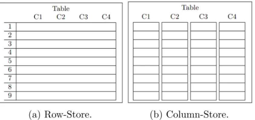
fragment the data. These different physical layouts are visualized in Figure 2-1.
Row Storage Databases fragment tables horizontally. In this storage model,
(a) Row-Store. (b) Column-Store.
Figure 2-1: Physical layout of row-store and column-store databases.
that operations on individual tuples are very efficient, as the data for a single tuple
is tightly packed at a single location. The main drawback of this approach is that
columns cannot be loaded individually from disk, as the values of a single column are
surrounded by the values of the other columns. Because of this, unused columns in the
table definition will affect query performance. When a query only operates on a subset
of the columns of a table, the entire table must be loaded from disk regardless. This
is especially relevant for OLAP-style queries that only touch a handful of columns in
large tables with hundreds or even thousands of columns.
Column Storage Databases fragment tables vertically. In this storage model,
the data of the individual columns is tightly packed. The advantages of this approach
are two-fold: (1) the columns can be loaded and used individually, which means we do
not need to load in any unused columns from disk, and (2) packing data of individual
columns together leads to significantly better compression. The trade-off, however,
is that reconstructing tuples is costly as the values of individual tuples are spread
out over different memory locations. As a result, operations on individual tuples are
expensive. As these types of operations are typically performed in OLTP workloads,
column storage lends itself towards OLAP workloads.
2.4
Database Processing Models
The processing model of the database heavily influences the design and performance of
between the database and the user-defined function. The processing model is closely
related to the physical storage of the database.
Tuple-at-a-Time Processing is the standard processing model used by most
disk-based systems. In this processing model, the individual rows of the database are
processed one by one from the start of the query to the end of the query.
The primary advantage of this processing model is that the system does not need to
keep large intermediates in memory. In extremely low memory situations, processing
queries in this fashion is often the only possibility. However, in situations where many
rows are processed the tuple–at–a–time processing model suffers heavily from high
interpretation overhead. This approach is used by PostgreSQL, MySQL and SQLite.
Operator–at–a–Time Processing is an alternative query processing model.
Instead of processing the individual tuples one by one, the individual operators of the
query are executed on the entire columns in order. As the operators process entire
columns at a time, the function call overhead of this processing model is minimal.
The main drawback of this processing model is the materialization cost of the
intermediates of the operators. In the tuple-at-a-time processing model, a single tuple
is processed from start to finish before the query processor moves on to the next tuple.
By contrast, in the operator–at–a–time processing model, the operator processes the
entire column at once before moving on to the next operator. Because of this, the
intermediate result of every operator has to be materialized into memory so the result
can be used by the next operator. As these intermediate results are the result of an
entire column being processed they can take up a significant amount of memory. This
approach is used by MonetDB.
Vectorized Processing is a hybrid processing model that sits between the
tuple-at-a-time and the operator–at–a–time models. It avoids high materialization costs by
operating on smaller chunks of rows at a time, while also avoiding overhead from a
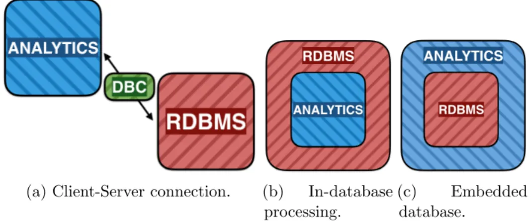
(a) Client-Server connection. (b) In-database processing.
(c) Embedded database.
Figure 2-2: Different ways of connecting external programs with a database manage-ment system.
3
Database Connectivity
While RDBMSs are very powerful, SQL is not a general purpose language. As such, it
is necessary for clients to write their actual application code in a different programming
language and communicate with the RDBMS in order to exchange data between the
application and the database management system.
As the focus of this work is on combining a RDBMS with analytical tools, we
focus especially on users wanting to use analytical tools (e.g. Python or R programs)
for the purpose of performing analysis on large amounts of data that reside in the
RDBMS. Figure 2-2 shows the three main methods in which a relational database
can be combined with an analytical tool. In this section, we will describe each of
these methods and discuss how they operate from both a usability and a performance
perspective.
3.1
Client-Server Connection
The standard method of combining a standalone program with a RDBMS is through
a client-server connection. This is visualized in Figure 2-2a. The database server is
completely separate from the analytical tool. It runs as either a separate process on the
same machine or on a different machine entirely. The analytical tool communicates with
interface (API). After an initial authentication phase, the client can issue a query to
the database server. The server will then execute the query. Afterwards, the result
of the query will be serialized and written to the client over the socket. Finally, the
client will deserialize the result.
The main advantage to this approach is that it is mostly database agnostic, as the
standardized ODBC [32] or JDBC [24] connectors can be used to connect to almost
every database. In addition, it is relatively easy to integrate into existing pipelines as
loading from flat files can be replaced by loading from a database without having to
modify the rest of the pipeline.
However, this approach is problematic when the client wants to run their analysis
pipelines on a a large amount of data. The time spent on serializing large result sets
and transferring them from the server to the client can be a significant bottleneck. In
addition, this approach requires the full dataset to fit inside the clients’ (often limited)
memory.
3.2
In-Database Processing
In order to avoid the cost of exporting the data from the database, the analysis can be
performed inside the database server. This method, known as in-database processing,
is shown in Figure 2-2b.
In-database processing can be performed in a database-agnostic way by rewriting
the analysis pipeline in a set of standard-compliant SQL queries. However, most
data analysis, data mining and classification operators are difficult and inefficient to
express in SQL. The SQL standard describes a number of built-in scalar functions
and aggregates, such as AVG andSUM [43]. However, this small number of functions
and aggregates is not sufficient to perform complex data analysis tasks [86].
Instead of writing the analysis pipelines in SQL, defined functions or
user-defined aggregates in procedural languages such as C/C++ can be used to implement
classification and machine learning algorithms. This is the approach taken by
Heller-stein et al. [36]. However, these functions still require significant rewrites of existing
user-defined functions in these languages require in-depth knowledge of the database
internals and the execution model used by the database [14].
3.3
Embedded Databases
Both the client-server model and in-database processing require the user to maintain a
running database server. This requires significant manual effort from the user, as the
database server must be installed, tuned and continuously maintained. For small-scale
data analysis, the effort spent on maintaining the database server often negates the
benefits of using one.
Embedding the database system inside the client program, as shown in Figure 2-2c,
is more applicable for these use cases. As the database can be installed and run from
within the client program, maintaining and setting up the database is much simpler
than with standalone database servers. As the database resides directly inside the
client process, the cost of transferring data between the client and the database server
is negated. The primary disadvantage of this solution is that only a single client can
have access to the data stored inside the database server.
4
MonetDB
MonetDB is an open source column-store RDBMS that is designed primarily for data
warehouse applications. In these scenarios, there are frequent analytical queries on the
database, often involving only a subset of the columns of the tables, and unlike typical
transactional workloads, insertions and updates to the database are infrequent and
in bulk or do not occur at all. The core design of MonetDB is described in Idreos et
al. [41]. However, since this publication a number of core features have been added to
MonetDB. In this section, we give a brief summary of the internal design of MonetDB
and describe the features that have been added to MonetDB since.
Data Storage. MonetDB stores relational tables in a columnar fashion. Every
column is stored either in-memory or on-disk as a tightly packed array. Row-numbers
their position in the tightly packed array. Missing values are stored as ”special“ values
within the domain of the type, i.e. a missing value in an INTEGERcolumn is stored internally as the value −231.
Columns that store variable-length fields, such as CLOBs or BLOBs, are stored
using a variable-sized heap. The actual values are inserted into the heap. The main
column is a tightly packed array of offsets into that heap. These heaps also perform
duplicate elimination if the amount of distinct values is below a threshold; if two fields
share the same value it will only appear once in the heap. The offset array will then
point to the same heap entry for the rows that share the same value.
Memory Management. MonetDB does not use a traditional buffer pool to
manage which data is kept in memory and which data is kept on disk. Instead, it relies
on the operating system to take care of this by using memory-mapped files to store
columns persistently on disk. The operating system then loads pages into memory as
they are used and evicts pages from memory when they are no longer being actively
used. This model allows it to keep hot columns loaded in memory, while columns that
are not frequently touched are off-loaded to disk.
Concurrency Control. MonetDB uses an optimistic concurrency control model.
Individual transactions operate on a snapshot of the database. When attempting to
commit a transaction, it will either commit successfully or abort when potential write
conflicts are detected.
Query Plan Execution. SQL is first parsed into a relational algebra tree and
then translated into an intermediate language called MAL (Monet Assembly Language).
MAL instructions process the data in a column-at-a-time model. Each MAL operator
processes the full column before moving on to the next operator. The intermediate
values generated by the operators are kept around in-memory if not too large, and
passed on to the next operator in the pipeline.
Optimizations happen at three levels. High level optimizations, such as filter push
down, are performed on the relational tree. Afterwards, the MAL code is generated
and further optimizations are performed, such as common sub-expression elimination.
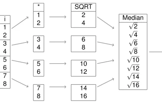
Figure 2-3: Parallel execution in MonetDB.
should be executed, such as which join implementation to use.
Parallel Execution. Initially, a sequential execution plan is generated.
Par-allelization is then added in the second optimization phase. The individual MAL
operators are marked as either “blocking” or “parallelizable”. The optimizers will
alter the plan by splitting up the columns of the largest table into separate chunks,
then executing the “parallelizable” operators once on each of the chunks, and finally
merging the results of these operators together into a single column before
execut-ing the “blockexecut-ing” operators. This is visualized in Figure 2-3 for the query SELECT MEDIAN(SQRT(i * 2)) FROM tbl.
The amount of chunks that are generated is decided by a set of heuristics based on
base table size, the amount of cores and the amount of available memory. The database
will attempt to generate chunks that fit inside main memory to avoid swapping, and
will attempt to maximize CPU utilization. In addition, the optimizer will not split up
small columns as the added overhead of parallel execution will not pay off in this case.
Automatic Indexing. In addition to allowing the user to manually build indices
Imprints [75] are a bitmap index that are used to assist in efficiently computing
point and range queries. The bitmap index holds, for each cache line, a bitmap
that contains information about the range of values in that cache line. They are
automatically generated for persistent columns when a range query is issued on a
specific column. They are then persisted on disk and used for subsequent queries on
that column. Imprints are destroyed when a column is modified.
Hash tables are also automatically created for persistent columns when they are
used in groupings or as join keys in equi-joins. These are also persisted on disk. Hash
tables are destroyed on updates or deletions to the column. Unlike imprints, however,
they are updated on appends to the tables.
Order Index. In addition to imprints and hash tables, MonetDB supports
creation of a sorted index that is not created automatically. It must be created using
the CREATE ORDER INDEX statement. Internally, the order index is an array of row numbers in the sort order specified by the user. The order index is used to speed up
point and range queries, as well as equi-joins and range-joins. Point and range queries
are answered by using a binary search on the order index. For joins, the order index
is used for a merge join.
5
Python
Python is a popular interpreted language, that is widely used by data scientists. It
is easily extensible through the use of modules. There are a wide variety of modules
available for common data science tasks, such asnumpy,tensorflow,scipy,sympy, sklearn,pandasandmatplotlib. These modules offer functions for high performance data analytics, data mining, classification, machine learning and plotting.
While there are various Python interpreters, the most commonly used interpreter
is the CPython interpreter. This interpreter is written in the language C, and provides
bindings that allow users to extend Python with modules written inC.
and a reference count. As every PyObject can be individually deleted by the garbage collector, every Python object has to be individually allocated on the heap.
The internal design of CPython has several performance implications that make
it unsuitable for working with large amounts of data. As every PyObject holds a reference count (64-bit integer) and type information (pointer), every object has 16
bytes of overhead on 64-bit systems. This means that a single 4-byte integer requires
20 bytes of storage. In addition, as everyPyObject has to be individually allocated on the heap, constructing a large amount of individual Python objects is very expensive.
Instead of storing every individual value as a Python object, packages intended
for processing large amounts of data work with NumPy arrays instead. Rather than
storing a single value as a PyObject, a NumPy array is a single PyObjectthat stores an array of values. This makes this overhead less significant, as the overhead is only
incurred once for every array rather than once for every value.
This solves the storage issue, but standard Python functions can only operate on
PyObjects. Thus if we want to actually operate on the individual values in Python, we would still have to convert each individual value to a PyObject.
The solution employed in Python (and other vector-based languages) is to have
vectorized functions that directly operate on all the data in an array. By using these
functions, the individual values are never loaded into Python. Instead, these vectorized
operations are written in C and operates directly on the underlying array. As these
functions operate on large chunks of data at the same time they also make liberal use
ofSIMD instructions, allowing these vectorized functions to be as fast as optimized C
Database Client-Server Protocols
1
Introduction
In Chapter 2, we described how client-server protocols can be used to combine
analytical tools with database servers. In this chapter, we dive further into the design
of client-server protocols in modern database systems. Specifically, we focus on the
manner in which result sets are (de)serialized and transported over a socket connection.
While the performance of result set (de)serialization is irrelevant for smaller result
sets, as the timing of the network will be dominated by the latency, the result set
(de)serialization becomes very relevant when the client wants to export a large amount
of data from the database system to a client program.
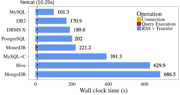
Figure 3-1 shows the impact that result set (de)serialization can have on query
time. It displays the time taken to run the SQL query “SELECT * FROM lineitem” using an ODBC connector and then fetching the results for various data management
systems. We see large differences between systems and disappointing performance
overall. Modern data management systems need a significant amount of time to
Netcat (10.25s) 170.9 170.9 170.9 189.6 189.6 189.6 629.9 629.9 629.9 221.2 221.2 221.2 686.5 686.5 686.5 101.3 101.3 101.3 391.3 391.3 391.3 202 202 202 MongoDB Hive MySQL+C MonetDB PostgreSQL DBMS X DB2 MySQL
0 200 400 600
Wall clock time (s)
Operation
Connection Query Execution RSS + Transfer
Figure 3-1: Wall clock time for retrieving the lineitem table (SF10) over a loopback connection. The dashed line is the wall clock time for netcat to transfer a CSV of the data.
located on the same machine.
1.1
Contributions
In this chapter, we investigate and benchmark the result set serialization methods used
by major database systems, and measure how they perform when transferring large
amounts of data in different network environments. We explain how these methods
perform result set serialization, and discuss the deficiencies of their designs that make
them inefficient for transfer of large amounts of data. We explore the design space of
result set serialization and investigate numerous techniques that can be used to create
an efficient serialization method. We extensively benchmark these techniques and
discuss their advantages and disadvantages.Finally, we propose a new column-based
serialization method that is suitable for exporting large result sets. We implement
our method in the Open-Source database systems PostgreSQL and MonetDB, and
demonstrate that it performs an order of magnitude better than the state of the art.
1.2
Outline
This chapter is organized as follows. In Section 2, we perform a comprehensive
analysis of state of the art in client protocols. We analyze techniques that can be
used to improve on the state of the art in Section 3. In Section 4, we describe
the implementation of our proposed protocol and perform an extensive evaluation
comparing our proposed protocol against the state of the art. We draw our conclusions
in Section 5.
2
State of the Art
Every database system that supports remote clients implements a client protocol.
Using this protocol, the client can send queries to the database server, to which the
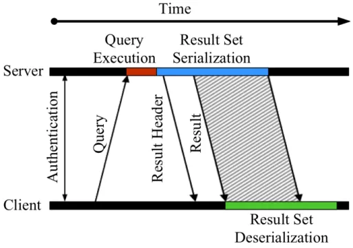
server will respond with a query result. A typical communication scenario between a
server and client is shown in Figure 3-2. The communication starts with authentication,
followed by the client and server exchanging meta information (e.g. protocol version,
database name). Following this initial handshake, the client can send queries to the
server. After computing the result of a query, (1) the server has to serialize the data
to the result set format, (2) the converted message has to be sent over the socket to
the client, and (3) the client has to deserialize the result set so it can use the actual
data.
The design of the result set determines how much time is spent on each step. If the
protocol uses heavy compression, the result set (de)serialization is expensive, but time
is saved sending the data. On the other hand, a simpler client protocol sends more
bytes over the socket but can save on serialization costs. The serialization format can
heavily influence the time it takes for a client to receive the results of a query. In this
section, we will take an in-depth look at the serialization formats used by state of the
Figure 3-2: Communication between a client and a server
2.1
Overview
To determine how state of the art databases perform at large result set export, we
have experimented with a wide range of systems: The row-based RDBMS MySQL [89],
PostgreSQL [76], the commercial systems IBM DB2 [91] and “DBMS X”. We also
included the columnar RDBMS MonetDB [41] and the non-traditional systems Hive [81]
and MongoDB [42]. MySQL offers an option to compress the client protocol using
GZIP (“MySQL+C”), this is reported separately.
There is considerable overlap in the use of client protocols. In order to be able to
re-use existing client implementations, many systems implement the client protocol of
more popular systems. Redshift [35], Greenplum [25], Vertica [49] and HyPer [58] all
implement PostgreSQL’s client protocol. Spark SQL [5] uses Hive’s protocol. Overall,
we argue that this selection of systems includes a large part of the database client
protocol variety.
Each of these systems offers several client connectors. They ship with a native
useful for creating a database and querying its state, however, it does not allow the
user to easily use the data in their own analysis pipelines.
For this purpose, there are database connection APIs that allow the user to query
a database from within their own programs. The most well known of these are the
ODBC [32] and JDBC [24] APIs. As we are mainly concerned with the export of large
amounts of data for analysis purposes, we only consider the time it takes for the client
program to receive the results of a query.
To isolate the costs of result set (de)serialization and data transfer from the other
operations performed by the database we use the ODBC client connectors for each of
the databases. For Hive, we use the JDBC client because there is no official ODBC
client connector. We isolate the cost of connection and authentication by measuring
the cost of theSQLDriverConnectfunction. The query execution time can be isolated by executing the query using SQLExecDirect without fetching any rows. The cost of result set (de)serialization and transfer can be measured by fetching the entire result
using SQLFetch.
As a baseline experiment of how efficient state of the art protocols are at transferring
large amounts of data, we have loaded thelineitemtable of the TPC-H benchmark [82] of SF10 into each of the aforementioned data management systems. We retrieved the
entire table using the ODBC connector, and isolated the different operations that
are performed when such a query is executed. We recorded the wall clock time and
number of bytes transferred that were required to retrieve data from those systems.
Both the server and the client ran on the same machine. All the reported timings
were measured after a “warm-up run” in which we run the same query once without
measuring the time.
As a baseline, we transfer the same data in CSV format over a socket using
the netcat (nc) [33] utility. The baseline incorporates the base costs required for transferring data to a client without any database-specific overheads.
Figure 3-1 shows the wall clock time it takes for each of the different operations
performed by the systems. We observe that the dominant cost of this query is the cost
the database and executing the query is insignificant compared to the cost of these
operations.
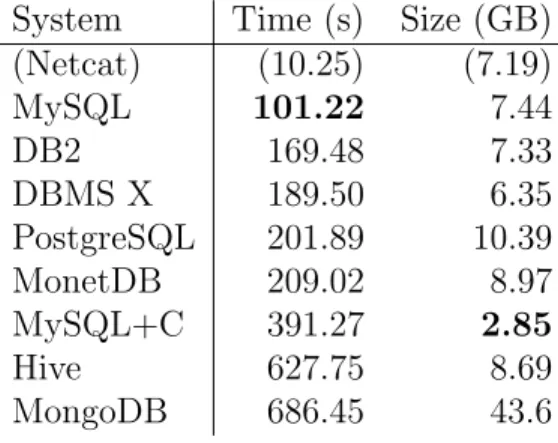
The isolated cost of result set (de)serialization and transfer is shown in Table 3.1.
Even when we isolate this operation, none of the systems come close to the performance
of our baseline. Transferring a CSV file over a socket is an order of magnitude faster
than exporting the same amount of data from any of the measured systems.
Table 3.1: Time taken for result set (de)serialization + transfer when transferring the SF10 lineitem table.
System Time (s) Size (GB) (Netcat) (10.25) (7.19) MySQL 101.22 7.44 DB2 169.48 7.33 DBMS X 189.50 6.35 PostgreSQL 201.89 10.39 MonetDB 209.02 8.97 MySQL+C 391.27 2.85
Hive 627.75 8.69 MongoDB 686.45 43.6
Table 3.1 also shows the number of bytes transferred over the loopback network
device for this experiment. We can see that the compressed version of the MySQL
client protocol transferred the least amount of data, whereas MongoDB requires
transferring ca. six times the CSV size. MongoDB suffers from its document-based
data model, where each document can have an arbitrary schema. Despite attempting
to improve performance by using a binary version of JSON (“BSON” [42]), each result
set entry contains all field names, which leads to the large overhead observed.
We note that most systems with an uncompressed protocol transfer more data
than the CSV file, but not an order of magnitude more. As this experiment was run
with both the server and client residing on the same machine, sending data is not the
main bottleneck in this scenario. Instead, most time is spent (de)serializing the result
● ● ● ● ● ● ● ● ● ● ● ● ● ● ● ● ● ● ● ● ● ● ● ● ● ● ● ● ● ● ● ●
DB2
DBMS X
Hive
MonetDB
MongoDB
MySQL
MySQL+C
PostgreSQL
10 1000.1 1.0 10.0 100.0
Latency (ms, log)
W
all clock time (s, log)
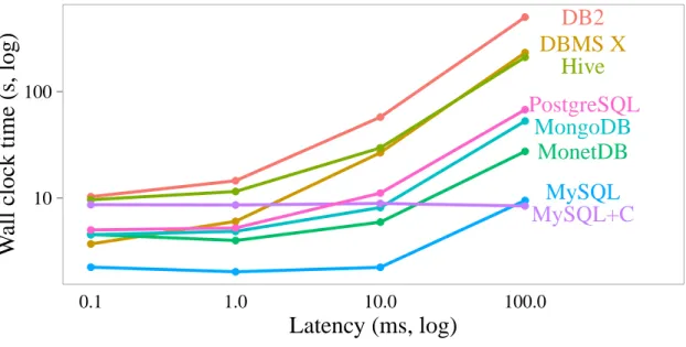
Figure 3-3: Time taken to transfer a result set with varying latency.
2.2
Network Impact
In the previous experiment, we considered the scenario where both the server and the
client reside on the same machine. In this scenario, the data is not actually transferred
over a network connection, meaning the transfer time is not influenced by latency
or bandwidth limitations. As a result of the cheap data transfer, we found that the
transfer time was not a significant bottleneck for the systems and that most time was
spent (de)serializing the result set.
Network restrictions can significantly influence how the different client protocols
perform, however. Low bandwidth means that transferring bytes becomes more costly;
which means compression and smaller protocols are more effective. Meanwhile, a higher
latency means round trips to send confirmation packets becomes more expensive.
To simulate a limited network connection, we use the Linux utility netem [39]. This utility allows us to simulate network connections with limitations both in terms
of bandwidth and latency. To test the effects of a limited network connection on the
different protocols, we transfer 1 million rows of the lineitemtable but with either limited latency or limited bandwidth.
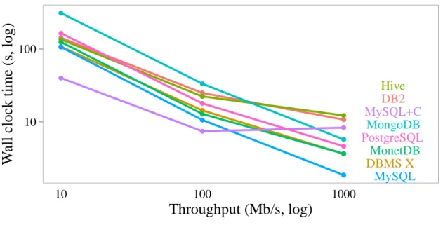
● ● ● ● ● ● ● ● ● ● ● ● ● ● ● ● ● ● ● ● ● ● ● ● DB2 DBMS X Hive MonetDB MongoDB MySQL MySQL+C PostgreSQL 10 100
10 100 1000
Throughput (Mb/s, log)
W
all clock time (s, log)
Figure 3-4: Time taken to transfer a result set with varying throughput limitations.
of the message size. High latency is particularly problematic when either the client
or the server has to receive a message before it can proceed. This occurs during
authentication, for example. The server sends a challenge to the client and then has
to wait a full round-trip before receiving the response.
When transferring large result sets, however, such handshakes are unnecessary.
While we expect a higher latency to significantly influence the time it takes to establish
a connection, the transfer of a large result set should not be influenced by the latency
as the server can send the entire result set without needing to wait for any confirmation.
As we filter out startup costs to isolate the result set transfer, we do not expect that
a higher latency will significantly influence the time it takes to transfer a result set.
In Figure 3-3, we see the influence that higher latencies have on the different
protocols. We also observe that both DB2 and DBMS X perform significantly worse
when the latency is increased. It is possible that they send explicit confirmation
messages from the client to the server to indicate that the client is ready to receive
the next batch of data. These messages are cheap with a low latency, but become
very costly when the latency increases.
influenced by a high latency. This is because, while the server and client do not
explicitly send confirmation messages to each other, the underlying TCP/IP layer
does send acknowledgement messages when data is received [66]. TCP packets are
sent once the underlying buffer fills up, resulting in an acknowledgement message. As
a result, protocols that send more data trigger more acknowledgements and suffer
more from a higher latency.
Throughput. Reducing the throughput of a connection adds a variable cost to
sending messages depending on the size of the message. Restricted throughput means
sending more bytes over the socket becomes more expensive. The more we restrict
the throughput, the more protocols that send a lot of data are penalized.
In Figure 3-4, we can see the influence that lower throughputs have on the different
protocols. When the bandwidth is reduced, protocols that send a lot of data start
performing worse than protocols that send a lower amount of data. While the
PostgreSQL protocol performs well with a high throughput, it starts performing
significantly worse than the other protocols with a lower throughput. Meanwhile, we
also observe that when the throughput decreases compression becomes more effective.
When the throughput is low, the actual data transfer is the main bottleneck and the
cost of (de)compressing the data becomes less significant.
2.3
Result Set Serialization
In order to better understand the differences in time and transferred bytes between
the different protocols, we have investigated their data serialization formats.
Table 3.2: Simple result set table.
INT32 VARCHAR10 100,000,000 OK
NULL DPFKG
For each of the protocols, we show a hexadecimal representation of Table 3.2
encoded with each result set format. The bytes used for the actual data are colored
44 50 46 4B 47
05
00
00
00
FF FF FF FF
44
00
00
00
10
00
02
00 00 00
04
05
F5
E1
00
00
00
00
02
4F 4B
44
00
00
00
0F
00
02
T
otal
Length
Field
Coun
t
Length
Field
1
Data
Field
1
Data
Field
2
Length
Field
2
Message
T
yp
e
Figure 3-5: PostgreSQL result set wire format
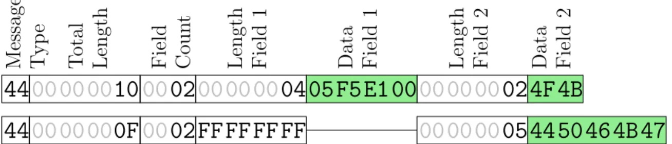
PostgreSQL. Figure 3-5 shows the result set serialization of the widely used
PostgreSQL protocol. In the PostgreSQL result set, every single row is transferred
in a separate protocol message [83]. Each row includes a total length, the amount of
fields, and for each field its length (−1 if the value is NULL) followed by the data. We can see that for this result set, the amount of per-row metadata is greater than the
actual data w.r.t. the amount of bytes. Furthermore, a lot of information is repetitive
and redundant. For example, the amount of fields is expected to be constant for an
entire result set. Also, from the result set header that precedes those messages, the
amount of rows in the result set is known, which makes the message type marker
redundant. This large amount of redundant information explains why PostgreSQL’s
client protocol requires so many bytes to transfer the result set in the experiment
shown in Table 3.1. On the other hand, the simplicity of the protocol results in low
serialization and deserialization costs. This is reflected in its quick transfer time if the
network connection is not a bottleneck.
44 50 46 4B 47
4F 4B
00
05
00
04
05
Data
Field
2
Data
Length
P
ac
k
et
Nr.
Data
Field
1
Length
Field
2
0D 00
07 00
31 30 30 30 30 30 30 30 02
FB
09
Length
Field
2
Length
Field
1
Figure 3-6: MySQL text result set wire format
MySQL. Figure 3-6 shows MySQL/MariaDB’s protocol encoding of the sample
data. The number of fields in a row is constant and defined in the result set header.
Each row starts with a three-byte data length. Then, a packet sequence number
(0-256, wrapping around) is sent. This is followed by length-prefixed field data. Field
lengths are encoded as variable-length integers. NULLvalues are encoded with a special field length, 0xFB. Field data is transferred in ASCII format. The sequence number is redundant here as the underlying TCP/Unix Sockets already guarantees that packets
arrive in the same order in which they were sent.
07
Length
Field
1
00
Length
Field
2
44 50 46 4B 47
02
Data
Field
2
Data
Field
1
07 02
4F 4B
05
C5 02
P
ac
k
et
Header
Figure 3-7: DBMS X result set wire format
DBMS X has a very terse protocol. However, it is much more computationally
heavy than the protocol used by PostgreSQL. Each row is prefixed by a packet header,
followed by the values. Every value is prefixed by its length in bytes. This length,
however, is transferred as a variable-length integer. As a result, the length-field is
only a single byte for small lengths. For NULL values, the length field is 0 and no actual value is transferred. Numeric values are also encoded using a custom format.
On a lower layer, DBMS X uses a fixed network message length for batch transfers.
This message length is configurable and according to the documentation, considerably
influences performance. We have set it to the largest allowed value, which gave the
best performance in our experiments.
MonetDB. Figure 3-8 shows MonetDB’s text-based result serialization format.
Here, the ASCII representations of values are transferred. This side-steps some issues
with endian-ness, transfer of leading zeroes and variable-length strings. Again, every
result set row is preceded by a message type. Values are delimited similar to CSV
files. A newline character terminates the result row. Missing values are encoded as
5B 20
44 50 46 4B 47
5B 20 4E 55
2C 09
09 5D 0A
31 30 30 30 30 30 30 30 30 2C 09 4F 4B
09 5D 0A
Line
T
yp
e
Data
Field
1
Field
Delim
iter
Line
End
Data
Field
2
4C 4C
Figure 3-8: MonetDB result set wire format
formatting characters (tabs and spaces), which serve no purpose here but inflate the
size of the encoded result set. While it is simple, converting the internally used binary
value representations to strings and back is an expensive operation.
1A
Field
Begin
00 00 00 00 00 00 00 00
3F
Field
Begin
1F
Field
Begin
28
List
Begin
00
Field
Stop
5F
AF
84
80
1F
Field
Begin
2B
List
Begin
05 44 50 46 4B 47
02 4F 4B
00
Field
Stop
00
Field
Stop
00 00 00
02
00
Field
Stop
58
Field
Begin
Start
Ro
w
O
ff
set
Colum
n
Coun
t
Data
Colum
n
1
Data
Colum
n
2
18
Field
Begin
00
01
NULL
Mask
Field
Length
02
00
Field
Stop
00
Figure 3-9: Hive result set wire format using “compact” Thrift encoding
Hive. Hive and Spark SQL use a Thrift-based protocol to transfer result sets [68].
Figure 3-9 shows the serialization of the example result set. From Hive version 2
onwards, a columnar result set format is used. Thrift contains a serialization method
for generic complex structured messages. Due to this, serialized messages contain
various meta data bytes to allow reassembly of the structured message on the client
side. This is visible in the encoded result set. Field markers are encoded as a single
This result set serialization format is unnecessarily verbose. However, due to the
columnar nature of the format, these overheads are not dependent on the number
of rows in the result set. The only per-value overheads are the lengths of the string
values and theNULL mask. The NULLmask is encoded as one byte per value, wasting a significant amount of space.
Despite the columnar result set format, Hive performs very poorly on our
bench-mark. This is likely due to the relatively expensive variable-length encoding of each
individual value in integer columns.
3
Protocol Design Space
In this section, we will investigate several trade-offs that must be considered when
designing a result set serialization format. The protocol design space is generally
a trade-off between computation and transfer cost. If computation is not an issue,
heavy-weight compression methods such as XZ [72] are able to considerably reduce
the transfer cost. If transfer cost is not an issue (for example when running a client on
the same machine as the database server) performing less computation at the expense
of transferring more data can considerably speed up the protocol.
In the previous section, we have seen a large number of different design choices,
which we will explore here. To test how each of these choices influence the performance
of the serialization format, we benchmark them in isolation. We measure the wall
clock time of result set (de)serialization and transfer and the size of the transferred
data. We perform these benchmarks on three datasets.
• lineitem from the TPC-H benchmark. This table is designed to be similar to
real-world data warehouse fact tables. It contains 16 columns, with the types of
either INTEGER, DECIMAL,DATE and VARCHAR. This dataset contains no missing values. We use the SF10 lineitem table, which has 60 million rows and is 7.2GB in CSV format.
of census survey responses. It consists of 274 columns, with the majority of type
INTEGER. 16.1% of the fields contain missing values. The dataset has 9.1 million rows, totaling 7.0GB in CSV format.
• Airline On-Time Statistics[62]. The dataset describes commercial air traffic punctuality. The most frequent types in the 109 columns are DECIMAL and VARCHAR. 55.2% of the fields contain missing values. This dataset has 10 million rows, totaling 3.6GB in CSV format.
3.1
Protocol Design Choices
Row/Column-wise. As with storing tabular data on sequential storage media, there
is also a choice between sending values belonging to a single row first versus sending
values belonging to a particular column first. In the previous section, we have seen
that most systems use a row-wise serialization format regardless of their internal
storage layout. This is likely because predominant database APIs such as ODBC and
JDBC focus heavily on row-wise access, which is simpler to support if the data is
serialized in a row-wise format as well. Database clients that print results to a console
do so in a row-wise fashion as well.
Yet we expect that column-major formats will have advantages when transferring
large result sets, as data stored in a column-wise format compresses significantly
better than data stored in a row-wise format [1]. Furthermore, popular data analysis
systems such as the R environment for statistical computing [69] or the Pandas Python
package [56] also internally store data in a column-major format. If data to be analysed
with these or similar environments is retrieved from a modern columnar or vectorised
database using a traditional row-based socket protocol, the data is first converted
to row-major format and then back again. This overhead is unnecessary and can be
avoided.
The problem with a pure column-major format is that an entire column is
trans-ferred before the next column is sent. If a client then wants to provide access to the
large result sets, this can be infeasible.
Our chosen compromise between these two formats is a vector-based protocol, where
chunks of rows are encoded in column-major format. To provide row-wise access, the
client then only needs to cache the rows of a single chunk, rather than the entire result
set. As the chunks are encoded in column-major order, we can still take advantage
of the compression and performance gains of a columnar data representation. This
trade-off is similar to the one taken in vector-based systems such as VectorWise [9].
Table 3.3: Transferring each of the datasets with different chunk sizes.
Chunksize Rows Time Size (GB) C. Ratio
Lineitem
2KB 1.4×101 55.9 6.56 1.38
10KB 7.1×101 15.2 5.92 1.80
100KB 7.1×10² 10.9 5.81 2.12 1MB 7.1×10³ 10.0 5.80 2.25
10MB 7.1×10⁴ 10.9 5.80 2.26
100MB 7.1×10⁵ 13.3 6.15 2.23
A
CS
2KB 1.0×100 281.1 11.36 2.06
10KB 8.0×100 46.7 9.72 3.18 100KB 8.5×101 16.2 9.50 3.68
1MB 8.5×10² 11.9 9.49 3.81
10MB 8.5×10³ 15.3 9.50 3.86
100MB 8.5×10⁴ 17.9 10.05 3.84
On
time
2KB 1.0×100 162.9 8.70 2.13 10KB 8.0×100 27.3 4.10 4.15
100KB 8.5×101 7.6 3.47 8.15
1MB 8.6×10² 6.9 3.42 9.80 10MB 8.6×10³ 6.2 3.42 10.24
100MB 8.6×10⁴ 11.9 3.60 10.84
Chunk Size. When sending data in chunks, we have to determine how large these
chunks will be. Using a larger chunk size means both the server and the client need to
allocate more memory in their buffer, hence we prefer smaller chunk sizes. However,
if we make the chunks too small, we do not gain any of the benefits of a columnar
protocol as only a small number of rows can fit within a chunk.
To determine the effect that larger chunk sizes have on the wall clock time
and compression ratio we experimented with various different chunk sizes using the