Research Article
A Novel Multiobjective Quantum-Behaved Particle Swarm
Optimization Based on the Ring Model
Di Zhou,
1Yajun Li,
1Bin Jiang,
1and Jun Wang
2,3,41School of Design Art & Media, Nanjing University of Science and Technology, China
2School of Digital Media, Jiangnan University, China
3Department of Radiology and BRIC, University of North Carolina at Chapel Hill, Chapel Hill, NC, USA
4Fujian Provincial Key Laboratory of Information Processing and Intelligent Control, Minjiang University, Fuzhou, China
Correspondence should be addressed to Di Zhou; [email protected]
Received 20 August 2016; Revised 26 September 2016; Accepted 10 October 2016 Academic Editor: Cheng-Tang Wu
Copyright © 2016 Di Zhou et al. This is an open access article distributed under the Creative Commons Attribution License, which permits unrestricted use, distribution, and reproduction in any medium, provided the original work is properly cited.
Due to its fast convergence and population-based nature, particle swarm optimization (PSO) has been widely applied to address the multiobjective optimization problems (MOPs). However, the classical PSO has been proved to be not a global search algorithm. Therefore, there may exist the problem of not being able to converge to global optima in the multiobjective PSO-based algorithms. In this paper, making full use of the global convergence property of quantum-behaved particle swarm optimization (QPSO), a novel multiobjective QPSO algorithm based on the ring model is proposed. Based on the ring model, the position-update strategy is improved to address MOPs. The employment of a novel communication mechanism between particles effectively slows down the descent speed of the swarm diversity. Moreover, the searching ability is further improved by adjusting the position of local attractor. Experiment results show that the proposed algorithm is highly competitive on both convergence and diversity in solving the MOPs. In addition, the advantage becomes even more obvious with the number of objectives increasing.
1. Introduction
Optimization problems with more than one objective are rather common in real-world practice, such as information system design [1], reservoir flood control operation (RFCO) problem [2], community detection [3] in social networks, and battery hybrid storage system optimization problems [4]. In such multiobjective optimization problems (MOPs), the objectives to be optimized are normally in conflict with each other, which means there is no unique solution to these problems. Instead, we are supposed to find Pareto opti-mal solutions that represent the best possible compromises among all the objectives.
In recent years, due to their population-based nature, a variety of evolutionary algorithms are applied to address the MOPs. Among these algorithms, particle swarm opti-mization (PSO) has attracted great interest for its relatively simple operation and competitive performance. Since the
first multiobjective PSO (MOPSO) proposed in 1999 [5], more than fifty variants of MOPSOs have been reported in literature, among which OMOPSO [6] proposed by Sierra and Coello is one of the most representative methods. Sierra and Coello [7] had given a survey of the existing studies on OMOPSOs before 2006, and the state-of-the-art MOPSOs are summarized by Zhou et al. [8]. Since classical PSO is designed for single-objective optimization problems and cannot be applied to multiobjective optimization problems directly, most of the existing studies have focused on how to extend PSO to its multiobjective versions, such as researches on how to select the global and local best particles [9–11], as well as how to maintain good points found so far.
However, as proved by Van Den Bergh [12], the classical PSO is not a global search algorithm, not even a local one, according to the convergence criteria provided by Solis and Wets [13]. Therefore, MOPSOs, which are derived from PSO, are unable to converge to global optima.
Quantum-behaved particle swarm optimization (QPSO) [14], first introduced by Sun et al. in 2004, is a new population-based algorithm, which is inspired by quantum mechanics and the trajectory analysis of PSO. Besides the
introduction of mean best position (mbest), the particles in
QPSO are assumed to follow a double exponential
distribu-tion in a quantum𝛿 potential well around its local focus
when a new position is sampled, which is the most significant difference between QPSO and PSO. Therefore, QPSO needs no velocity vectors for particles at all. Since its first proposal, QPSO has shown its success in solving a wide range of single-objective optimization problems [15–17].
In contrast with PSO, the global convergence of QPSO can be guaranteed if the contraction-expansion (CE) coef-ficient of the algorithm is properly selected [18, 19]. Sun et al. proved that the QPSO is a form of contraction mapping on the probability metric space and its orbit is probabilistic bounded, and, in turn, the algorithm converges asymptoti-cally to the global optimum. It is the exact reason why QPSO outperforms PSO as well as most of the other evolutionary algorithms.
Although QPSO has been successfully applied in con-ventional single-objective optimization problems due to its global convergence and easy control, it is rarely used in solving multiobjective optimization problems [20, 21]. Although the QPSO algorithm can be global convergent, the CE coefficient is generally selected to be relatively small in order to accelerate the convergence of the algorithm for real-word problems so that premature convergence can result when the algorithm is performed for the MOPs. To eliminate this defect, we propose a novel position-update mechanism based on the ring model and combine it with the classical QPSO. This leads to MOQPSOr, an enhanced QPSO method which can be applied to the multiobjective optimization problems. The combination of the ring model with QPSO has several merits. Firstly, it employs a novel communication mechanism between particles using the ring model. This modification enables the swarm to have much larger mutate scope compared to the original QPSO, which effectively slows down the descent speed of the swarm diversity, solving the problem of premature caused by the quick convergence when applying QPSO directly into multiobjective optimization. Secondly, in this ring model, by adjusting the position of local attractor, the global searching ability is enhanced at the beginning of iteration, while the local searching ability is enhanced in the later stage of iteration. By employing this novel position-update strategy based on the ring model, the efficiency of MOQPSOr on multiobjective optimization is further improved, since there is no need for any additional mutation operation.
The rest of the paper is organized as follows: After a brief introduction of the background of PSO and QPSO in Section 2, a novel ring model for position update is proposed in Section 3 and a new version of multiobjective quantum-behaved particle swarm optimization algorithm (MOQPSOr) is presented by integrating the new position-update strategy into it accordingly. Numerical tests and performance compar-ison on 12 benchmark functions are provided in Section 4. Finally, the paper is concluded in Section 5.
2. Related Work
Being a heuristic search technique that simulates the sociol-ogy behaviour of an organism, particle swarm optimization (PSO) [22, 23] has become one of the most popular methods in the fields of evolutionary computation. In PSO, each particle represents a candidate solution to the problem and
flies through aD-dimensional search space according to the
following position-update equation:
𝑉𝑖,𝑗(𝑡 + 1) = 𝜔 ⋅ 𝑉𝑖,𝑗(𝑡) + 𝑐1⋅ 𝑟1,𝑗(𝑡)
⋅ [𝑝best𝑖,𝑗(𝑡) − 𝑋𝑖,𝑗(𝑡)] + 𝑐2⋅ 𝑟2,𝑗(𝑡)
⋅ [𝑔best𝑗(𝑡) − 𝑋𝑖,𝑗(𝑡)] ,
𝑋𝑖(𝑡 + 1) = 𝑋𝑖(𝑡) + 𝑉𝑖(𝑡 + 1) ,
(1)
where the current position and velocity of𝑖th particle at the
tth iteration are represented, respectively, as𝑋𝑖(𝑡) = (𝑋𝑖,1(𝑡),
𝑋𝑖,2(𝑡), . . . , 𝑋𝑖,𝐷(𝑡))and 𝑉𝑖(𝑡) = (𝑉𝑖,1(𝑡), 𝑉𝑖,2(𝑡), . . . , 𝑉𝑖,𝐷(𝑡)).
𝑝bestiis the best previous position of particlei, while𝑔best
is the position of the best particle in the whole swarm.
The parameters 𝑟1 and 𝑟2 are different random numbers
distributed uniformly on (0,1), and 𝑐1 as well as 𝑐2 denote
the acceleration coefficients that typically are both set to a value of 2.0, which implies that the “social” and “cognition” parts have the same influence on the velocity update. The
parameter𝜔is known as the inertia weight and is usually set
to a positive value chosen from a linear or nonlinear function of the iteration number.
Compared with PSO, the most significant advantage of QPSO is that its global convergence can be theoretically guaranteed [18]. In addition, QPSO is much easier to be con-trolled, benefiting from the fact that it only has one parameter. Trajectory analyses demonstrated the fact that convergence of the whole particle swarm may be achieved if each particle
converges to its local attractor𝑝𝑖= (𝑝𝑖1, 𝑝𝑖2, . . . , 𝑝𝑖𝐷)[24]:
𝑝𝑖,𝑗(𝑡)
= [𝑐1⋅ 𝑟1,𝑗(𝑡) ⋅ 𝑝best𝑖,𝑗(𝑡) + 𝑐2⋅ 𝑟2,𝑗(𝑡) ⋅ 𝑔best𝑗(𝑡)] [𝑐1⋅ 𝑟1,𝑗(𝑡) + 𝑐2⋅ 𝑟2,𝑗(𝑡)] ,
or: 𝑝𝑖,𝑗(𝑡) = 𝜑 ⋅ 𝑝best𝑖,𝑗(𝑡) + (1 − 𝜑) ⋅ 𝑔best𝑗(𝑡) ,
(2)
where 𝜑 is a sequence of uniformly distributed random
numbers in (0,1).
Unlike PSO, each individual particle in QPSO moves
in the search space with a 𝛿potential on each dimension,
of whose center is point 𝑝𝑖,𝑗. When a particle 𝑥𝑖 evolves
its position in this𝛿potential, the new position𝑋𝑖(𝑡 + 1)
is subject to an exponential distribution whose probability density function is
𝐹 (𝑋𝑖(𝑡 + 1) − 𝑝𝑖(𝑡))
= 1
𝐿𝑖(𝑡)exp(−2 𝑋𝑖
(𝑡 + 1) − 𝑝𝑖(𝑡)
𝐿𝑖(𝑡) ) ,
where 𝐿𝑖 determines the distribution scope. In QPSO, the distribution scope of each particle is set elaborately to relate to its relative position in the whole swarm:
𝐿𝑖,𝑗= 2𝛽 ⋅ 𝑚best𝑗(𝑡) − 𝑋𝑖,𝑗(𝑡) , (4)
wherembest is the mean of the personal best positions among
all particles:
𝑚best(𝑡) = (𝑚best1(𝑡) , 𝑚best2(𝑡) , . . . , 𝑚best𝐷(𝑡))
= (𝑀1∑𝑀
𝑖=1
𝑝best𝑖,1(𝑡) , 1
𝑀
⋅∑𝑀
𝑖=1
𝑝best𝑖,2(𝑡) , . . . , 1
𝑀
𝑀
∑
𝑖=1
𝑝best𝑖,𝐷(𝑡)) .
(5)
In this way, particles far away from the center of the whole swarm will have a larger searching scope, while those particles close to the middle can only search in a relatively limited small space. Therefore, the position of the particle in QPSO is updated according to the following iteration equation:
𝑋𝑖,𝑗(𝑡 + 1) = 𝑝𝑖,𝑗± 𝛽 ⋅ 𝑚best𝑗− 𝑋𝑖,𝑗(𝑡) ⋅ln(1
𝜇) , (6)
where𝜇is a random number uniformly distributed in (0,1)
and𝛽is called Contraction-Expansion Coefficient, which is
employed to control the convergence speed of the algorithm.
As proved by Sun et al. [14],𝛽must be set as𝛽 < 1.782to
guarantee convergence of the particle.
3. Proposed Method
3.1. Novel Ring Model Based Position-Update Strategy. From the perspective of both empirical evidence and theory analy-sis, the global search ability as well as the convergence rate of QPSO and its variants has been fully discovered on the single-objective optimization problems. However, this advantage of QPSO leads to premature convergence when it is applied directly to the multiobjective optimizations. Without the loss of generality, a multiobjective optimization problem can be formulated as follows:
min𝐹 (𝑥) = [𝑓1(𝑥) , 𝑓2(𝑥) , . . . , 𝑓𝑀(𝑥)]𝑇, (7)
where𝑓𝑖 (𝑖 = 1, 2, . . . , 𝑀)are the objective functions, while
𝑥 = [𝑥1, 𝑥2, . . . , 𝑥𝐷]𝑇 ∈ Ωis the vector of decision variable. The optimization performance is generally measured by two aspects: closeness to the ideal Pareto front and distribution of the approximated solutions [8]. However, the quick con-vergence property of QPSO is apt to lead rapid decline of the swarm’s diversity, which becomes a serious problem that must be addressed when it is extended into multiobjective optimization.
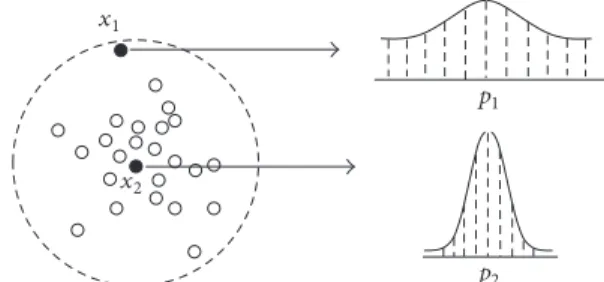
Each particle in QPSO is located in an exponential
distributed potential, with the center 𝑝𝑖 and distribution
scope 𝐿𝑖, respectively. Figure 1 illustrates the relationship
between the particle position and its distribution scope in
x1
x2
p1
p2
Figure 1: The dependence of the search scope of the particle on the distance of the particle from the mean best position.
xi−1
xi+1
xi
Figure 2: All the particles in the swarm are arranged in circle in MOQPSOr.
QPSO. Here, 𝑥1 represents the particle far away from the
mean best position (mbest) of the swarm and its
corre-sponding distribution at next iteration with the center 𝑝1
visualised on upper right;𝑥2 denotes the particle near the
mean best position of the swarm with𝑝2being the center of
the exponential distribution of its position at next iteration. According to the iteration equation of QPSO, we can see in
the figure that𝑥2has a much smaller variation scope than𝑥1.
That is, the closer𝑥𝑖 to the mean best position, the smaller
the scope of the variation. Only those particles away from the
mbest, like𝑥1, have the large variation scope. That implies
that, in original QPSO, a certain number of particles in the swarm are supposed to have small, or even very close to zero, distribution scopes.
In order to control the descent speed of the swarm diversity, we propose a novel position-update strategy based
on the ring model. In this model, for a swam with 𝑀
particles, all the particles are arranged in a circle like Figure 2,
numbered as𝑥1, 𝑥2, . . . , 𝑥𝑖−1, 𝑥𝑖, 𝑥𝑖+1, . . . , 𝑥𝑀. Different from
the way of deciding particle’s variation scope according to its location in the swarm in original QPSO, in our proposed
method, when the particle𝑥𝑖evolves, its variation scope is
decided by the distance to its next-numbered particle𝑥𝑖+1.
Accordingly, for the iteration equation of particle 𝑥𝑖, we
replace mbest by 𝑝best𝑖+1, which represents the personal
best position of particle𝑥𝑖+1. Since particles in the swarm
are distributed randomly and independently, the position of
𝑥𝑖+1can locate everywhere in the search space theoretically.
0 0.1 0.2 0.3 0.4 0.5 0.6 0.7 0.8 0.9 1
r p
gbest
pbest
(a) The location of local attractor𝑝when𝛼 = 0.3
0 0.1 0.2 0.3 0.4 0.5 0.6 0.7 0.8 0.9 1
r p
gbest
pbest
(b) The location of local attractor𝑝when𝛼 = 3
Figure 3: The relationship between the location of the local attractor𝑝and the value of𝑟for different values of𝛼.
with large scopes. Therefore, by this novel position-update strategy, the swarm of MOQPSOr can mutate more than the original QPSO, which subsequently leads to the slowdown of the descent speed of the swarm diversity.
In terms of the local attractor 𝑝𝑖, in QPSO, it is set to
lie uniform-randomly in the hyperrectangle withpbestiand
𝑔best being two ends of its diagonal. Generally speaking,
the local searching ability will be enhanced when𝑝𝑖 moves
towards𝑔best, and when𝑝𝑖moves towardspbesti, the global
searching ability will be enhanced. Therefore, in MOQPSOr,
𝑝𝑖 is given larger probabilities locating near pbesti in the
beginning and near 𝑔best in the later stage of iteration,
respectively
Based on the above analysis, particles in MOQPSOr that move according to the position-updating strategy can be described as follows:
𝑋𝑖,𝑗(𝑡 + 1) = 𝑝𝑖,𝑗± 𝛽 ⋅ 𝑝best𝑖+1,𝑗(𝑡) − 𝑋𝑖,𝑗(𝑡)
⋅ln(1
𝜇) , 𝜇 ∼ 𝑈 (0, 1) ,
(8)
where:𝑝𝑖,𝑗= 𝑔best𝑗+ (𝑝best𝑖,𝑗− 𝑔best𝑗) ⋅ 𝑟𝛼,
𝑟 ∼ 𝑈 (0, 1) , (9)
where parameter𝛼is called Searching Coefficient, by
adjust-ing which, local attractor𝑝𝑖,𝑗can be controlled to appear near
pbesti,jor𝑔bestj. Figure 3 plots the distribution ofp’s location
formulated in (9), where the horizontal axis denotes the
random numberr and the vertical axis denotesp’s location
between pbest and 𝑔best. 𝛼 = 0.3 and 𝛼 = 3 are used
as examples to demonstrate situations when 𝛼 < 1 and
𝛼 > 1, respectively. From the red dotted lines, it could be
seen that when 𝛼 = 0.3, p has half probability to locate
in [𝑝best, 0.812𝑝best + 0.188𝑔best], which is much closer
topbest than to𝑔best. In Figure 3(b), when𝛼 = 3, phas
half probability to locate in[0.125𝑝best+ 0.875𝑔best, 𝑔best],
which is closer to𝑔best than to pbest. That is, when𝛼 <
1, the local attractor𝑝would appear near pbest with large
probability.The smaller the value of𝛼is,the closer the point
𝑝gathers towardspbest. On the contrary, when𝛼 > 1, p
would appear with large probability near𝑔best.The bigger
the value of𝛼is, the closer the point𝑝gathers towards𝑔best.
Therefore, the algorithm’s global searching ability could be
enhanced by setting𝛼 < 1, while the local searching ability
could be enhanced by setting𝛼 > 1.
3.2. Multiobjective QPSO with Ring Model (MOQPSOr). In MOQPSOr, we adopt the concept of crowding distance [25] for the leader selection. Whenever a leader particle needs to be selected as the global best position from the external archive, the crowding factor of each leader is calculated, followed by the subsequent selection by means of a binary tournament based on these crowding factors. A particle with larger crowding distance has more chances to be chosen as leader.
Crowding distance of each individual is also used to decide which leaders would keep over generations when the maximum external archive size is exceeded in MOQPSOr. The particle in the archive with the smallest crowding distance will be removed first whenever needed.
Since MOQPSOr could have already slowed down the descent speed of the swarm diversity by the novel position-update strategy based on ring model, there is no need for any additional mutation operation. The procedure of the MOQPSOr algorithm could be described as follows.
Step 1(initialization).
Step 1.1. Parameter settings are as follows: the swarm size
M, the external archive size 𝐸size, the stopping criterion
𝑇max, iteration time 𝑡 = 0, Searching Coefficient 𝛼, and
Step 1.2. Initialize the swarm randomly within the feasible
solution space𝑋 = (𝑋1, 𝑋2, . . . , 𝑋𝑀), as well as the personal
best positions𝑝best = (𝑝best1, 𝑝best2, . . . , 𝑝best𝑀), where
𝑝best𝑖= 𝑋𝑖, 𝑖 ∈ [1, 𝑀].
Step 1.3. Initialize the external archive𝐸as the nondominated
solution inpbest.
Step 2(termination). If termination condition is met, stop
and return all the individuals in the current𝐸. Otherwise, go
to Step 3.
Step 3(reproduction). For each particle𝑋𝑖, 𝑖 ∈ [1, 𝑀], note the following.
Step 3.1. Select a global best position𝑔besti from external
archive.
Step 3.2. Update position by (8) and (9).
Setp 3.3. Update personal best positionpbesti.
Step 4(external archive update).
Step 4.1. Consider𝐸(𝑡 + 1) = 𝐸(𝑡) ∪ 𝑝best.
Step 4.2. Remove dominated solutions in𝐸(𝑡 + 1).
Step 4.3. If the size of the current 𝐸 is larger than 𝐸size,
calculate the crowding distance of each individual inE, sort
them in descending order of crowding distance, and keep the
first𝐸sizeindividuals in𝐸(𝑡 + 1).
Step 5. Consider𝑡 = 𝑡 + 1; go to Step 2.
4. Experiments and Analysis
4.1. Test Functions. Walking-Fish-Group (WFG) [26], a well-designed multiobjective test suite which provides a truer means of assessing the performance of optimization algo-rithms on a wide range of different problems, is used to validate the performance of our approach in 2-objective space. Compared with the other two commonly used suite of ZDT [27] and DTLZ [28], WFG test suite is more challenging and contains a number of problems that exhibit properties not evident in ZDT and DTLZ, including nonseparable problems, deceptive problems, a truly degenerate problem, a mixed shape Pareto front problem, problems scalable in the number of position-related parameters, and problems with dependencies related to position and distance parameters.
Besides WFGs, another three 3-objective benchmark functions, which are acknowledged for the extreme difficulty to optimize in the DTLZ test suite, are also involved in the comparison test. DTLZ2 tests the ability of global conver-gence by providing a spherical Pareto front. DTLZ4 assesses the maintainability of a good distribution of solutions by generating a nonuniform distribution of points along the true Pareto front. The Pareto front of DTLZ7 is the intersection of a straight line and a hyperplane. All these twelve benchmark problems are listed in Table 1.
4.2. Performance Metrics. To assess the performance of algorithms in this experiment, three quality indicators are
considered: Additive Unary 𝜀-indicator (𝐼𝜀+1) [29],
hyper-volume (𝐼HV) [30], and the Inverted Generational Distance
(IGD) [31].
Additive Unary𝜀-Indicator(𝐼𝜀+1 ). It measures the convergence of the resulting Pareto fronts. A lower value indicates a better
approximation set. For an approximation setX, the additive
Unary𝜀-indicator is defined as [32]
𝐼𝜀+1 (𝑋) =inf 𝜀∈R{∀𝑧
2∈ 𝑃∃𝑧1∈ 𝑋 : 𝑧1≻ 𝑧2} ,
(10)
where𝑃is the ideal Pareto front.
Hypervolume (𝐼𝐻𝑉). This metric measures both convergence
and diversity of the solutions. The higher the𝐼HVvalues are,
the better the algorithm performs. Generally speaking, the hypervolume measures the volume of the space dominated by
the approximation set, bounded by a reference point.𝐼HV(𝑋)
of an approximation set𝑋can be mathematically defined as
𝐼HV(𝑋) = Λ ( ⋃
(𝑥1,...,𝑥𝑑)∈𝑋
[𝑟1, 𝑥1] × ⋅ ⋅ ⋅ × [𝑟𝑑, 𝑥𝑑]) , (11)
where𝑟 = (𝑟1, 𝑟2, . . . , 𝑟𝑑)is the reference point andΛis the
usual Lebesgue measure.
Inverted Generational Distance (IGD). Inverted Generational Distance is the average distance from every solution in the reference set to the nearest solution in the approximation set; it, therefore, reflects convergence of the solutions. The fewer the IGD values, the better the algorithm’s performance.
The IGD metric is calculated for the solution set𝑋using the
reference point set𝑍as follows:
IGD(𝑍, 𝑋) = 1
|𝑍|
|𝑍|
∑
𝑖=1 |𝑋| min
𝑗=1 𝑑 (𝑧𝑖, 𝑥𝑗) , (12)
where 𝑑(𝑧𝑖, 𝑥𝑗) is the distance between 𝑧𝑖 and 𝑥𝑗 in the
objective space.
4.3. Algorithm for Comparison and Parameter Setting. In this experiment, five state-of-the-art multiobjective optimization algorithms are chosen for comparison, including the most efficient and widely used multiobjective particle swarm opti-mizer OMOPSO [6] and another two well-known PSO-based
multiobjective optimization algorithms:𝜎MOPSO [33] and
pdMOPSO [34], as well as two competitive evolutionary multiobjective optimizers: NSGA-II [25] and PESA-II [35].
To make a fair comparison, the population size and the leader archive in MOQPSOr and all the other five comparison algorithms are fixed to 100 for all test instances. The stopping condition is set to 250 iterations, which means a total of 25000
function evaluations. For MOQPSOr, 𝛼 increases linearly
from 0.6 to 1.2, and𝛽is set to 0.3. For OMOPSO,𝜎MOPSO,
and pdMOPSO, the sets of 𝐶1, 𝐶2, and 𝜔, as well as the
T a b le 1: D es cr ipt ion of th e te st fu n ct io ns . Co d e Ob jecti ve fu n cti o n s F ea tur e O b jec ti ve s WFG1 min 𝑓𝑚=1:𝑀 −1 (𝑥 )=𝑥 𝑀 +2 𝑚 ( 𝑀− 𝑚 ∏ 𝑖=1 (1− cos ( 𝑥𝑖
𝜋 ))) 2
⋅( 1− sin ( 𝑥𝑀− 𝑚 +1 𝜋 2 )) M ix ed , co n vex/co n ca ve ,U nimo d al ,s ep ar ab le 2 min 𝑓𝑀 (𝑥) = 𝑥𝑀 +2 𝑚 (1−𝑥 1 − cos (2𝐴𝜋 𝑥1 +𝜋 /2 ) 2𝐴𝜋 ) 𝛼 𝑥={ 𝑥1 ,...,𝑥 𝑀 }= { max (𝑡
𝑝 𝑀,𝐴
1
)(
𝑡
𝑝 𝑀−
0.5) + 0.5, .. ., max (𝑡
𝑝 𝑀,𝐴
𝑀− 1 )( 𝑡 𝑝 𝑀− 1 − 0.5) + 0.5, 𝑡
𝑝 𝑀}
𝑡
𝑝 =
{𝑡
𝑝 1,...,𝑡
𝑝 𝑀}
← 𝑡 𝑝−1 ← ⋅⋅ ⋅← 𝑡 1 𝑡 1 𝑖=1:𝑘 =𝑦 𝑖 𝑡 1 𝑖=𝑘+1:𝑛 =𝑠 line ar (𝑦𝑖 ,0.35) 𝑡 2 𝑖=1:𝑘 =𝑦 𝑖 𝑡 2 𝑖=𝑘+1:𝑛 =𝑏 fla t (𝑦𝑖 ,0.8, 0.75, 0.85) 𝑡 3 𝑖=1:𝑛 =𝑏 p oly (𝑦𝑖 ,0.02) 𝑡 4 𝑖=1:𝑀 −1 = 𝑟 sum ({𝑦 (𝑖−1)𝑘/(𝑀 −1)+1 ,...,𝑦 𝑖𝑘/(𝑀 −1) },{ 2( (𝑖−1 )𝑘 (𝑀−1 ) + 1),..., 2𝑖𝑘 (𝑀−1 ) }) 𝑡 4 𝑖=𝑀 =𝑟 sum ({ 𝑦𝑘+1 ,...,𝑦 𝑛 }, {2 (𝑘+1 ),...,2 𝑛} ) WFG2 𝑓𝑚=1:𝑀 −1 an d 𝑡 1are as th o se fr om W F G 1, C o n vex,dis co nnec te d ,U nimo d al ,m ul ti mo dal ,no n sepa ra b le 2 min 𝑓𝑀 (𝑥) = 𝑥𝑀 +1−( 𝑥1 ) 𝛼 cos 2 (𝐴(𝑥 1 ) 𝛽 𝜋) , 𝛼 =𝛽=1 , 𝐴 =5 𝑡 2 𝑖=1:𝑘 =𝑦 𝑖 𝑡 2 𝑖=𝑘+1:𝑘+𝑙/2 =𝑟 no ns ep ({𝑦 𝑘+2(𝑖−𝑘)−1 ,𝑦𝑘+2(𝑖−𝑘) },2 ) 𝑡 3 𝑖=1:𝑀 −1 =𝑟 sum ({𝑦 (𝑖−1)𝑘/(𝑀 −1)+1 ,𝑦𝑖𝑘/(𝑀 −1) }, {1 ,...,1 }) 𝑡
3 𝑀=𝑟
sum ({ 𝑦𝑘+1 ,...,𝑦 𝑘+𝑙/2 }, {1 ,...,𝑙 }) 𝑡 4 𝑖=𝑀 =𝑟 sum ({ 𝑦𝑘+1 ,...,𝑦 𝑛 },{2 (𝑘+1 ),...,2 𝑛} ) WFG3 min 𝑓1 (𝑥) = 𝑥𝑀 +2 𝑚 𝑀− 1 ∏ 𝑖=1 𝑥𝑖 L iner ,deg enera te ,unimo d al ,no n se pa ra b le 2 min 𝑓𝑚=2:𝑀 −1 (𝑥) = 𝑥𝑀 +2 𝑚 ( 𝑀− 𝑚 ∏ 𝑖=1 𝑥𝑖 ) ⋅( 1−𝑥 𝑀− 𝑚 +1 ) min 𝑓𝑀 (𝑥) = 1 − 𝑥1 𝑡 1:3 are as th o se fr om W F G 2 WFG4 min 𝑓1 (𝑥 )=𝑥 𝑀 +2 𝑚 ( 𝑀− 1 ∏ 𝑖=1 sin ( 𝑥𝑖
𝜋 )) 2
C o nca ve ,m u lt imo d al ,s epa ra b le 2 min 𝑓𝑚=2:𝑀 −1 (𝑥) = 𝑥𝑀 +2 𝑚 ( 𝑀− 𝑚 ∏ 𝑖=1 sin ( 𝑥𝑖
𝜋 ))⋅ 2
cos ( 𝑥𝑀− 𝑚 +1 𝜋 2 ) min 𝑓𝑀 (𝑥) = 𝑥𝑀 +2 𝑚 cos ( 𝑥1
𝜋 ) 2
𝑡 1 𝑖=1:𝑛 =𝑠 mu lt i (𝑦𝑖 ,30, 10, 0.35) 𝑡 2 𝑖=1:𝑀 −1 =𝑟 sum ({𝑦 (𝑖−1)𝑘/(𝑀 −1)+1 ,...,𝑦 𝑖𝑘/(𝑀 −1) }, {1 ,...,1 }) 𝑡
2 𝑀=𝑟
Ta b le 1: C o n ti n u ed . Co d e Ob jecti ve fu n cti o n s F ea tur e O b jec ti ve s WFG6 𝑓𝑚=1:𝑀 are as th o se fr om W F G 4 , 𝑡 1 as th os e fr o m W FG1, C o nca ve ,unimo d al ,no n se pa ra b le 2 𝑡 2 𝑖=1:𝑀 −1 =𝑟 no ns ep ({ 𝑦(𝑖−1)𝑘/(𝑀 −1)+1 ,...,𝑦 𝑖𝑘/(𝑀 −1) }, 𝑘 (𝑀−1 ) ) 𝑡 2 𝑀 =𝑟 no ns ep ({𝑦 𝑘+1 ,...,𝑦 𝑛 },𝑙 ) WFG7 𝑓𝑚=1:𝑀 are as th o se fr om W F G 4 , 𝑡 2 as 𝑡 1 fr o m W F G 1, 𝑡 3 as 𝑡 2 fr o m W F G 4 , C o nca ve ,unimo d al ,s epa ra b le 2 𝑡 1 𝑖=1:𝑘 =𝑏 pa ra m (𝑦𝑖 ,𝑟 sum ({𝑦 𝑖+1 ,...,𝑦 𝑛 }, {1 ,...,1 }), 0.98 49.98 ,0.02, 50) 𝑡 1 𝑖=𝑘+1:𝑛 =𝑦 𝑖 WFG8 𝑓𝑚=1:𝑀 are as th o se fr om W F G 4 , 𝑡 2 as 𝑡 1 fr o m W F G 1, 𝑡 3 as 𝑡 2 fr o m W F G 4 , C o nca ve ,unimo d al ,no n se pa ra b le 2 𝑡 1 𝑖=1:𝑘 =𝑦 𝑖 𝑡 1 𝑖=𝑘+1:𝑛 =𝑏 pa ra m (𝑦𝑖 ,𝑟 sum ({𝑦 1 ,...,𝑦 𝑖−1 },{1 ,...,1 }), 0.98 49.98 ,0.02, 50) WFG9 𝑓𝑚=1:𝑀 are as th o se fr om W F G 4 , 𝑡 3 as 𝑡 2 fr o m W F G 6 , C o nca ve ,m u lt imo d al ,decep ti ve ,no n se p ara b le 2 𝑡 1 𝑖=1:𝑛−1 =𝑏 pa ra m (𝑦𝑖 ,𝑟 sum ({ 𝑦𝑖+1 ,...,𝑦 𝑛 }, {1 ,...,1 }) , 0.98 49.98 ,0.02, 50 ) 𝑡 1 𝑖=𝑛 =𝑦 𝑛 𝑡 2 𝑖=1:𝑘 =𝑠 decep t (𝑦𝑖 ,0.35, 0.001, 0.05) 𝑡 2 𝑖=𝑘+1:𝑛 =𝑠 mu lt i (𝑦𝑖 ,30, 95, 0.35) D T LZ2 min 𝑓1 (𝑥 )=( 1 + 𝑔 (𝑥𝑀 )) 𝑀− 1 ∏ 𝑖=1 cos ( 𝑥𝑖
𝜋 ) 2
min 𝑓𝑚=2:𝑀 −1 (𝑥) = (1 + 𝑔 (𝑥𝑀 )) sin ( 𝑥𝑀− 𝑚 +1 𝜋 2 ) 𝑀− 𝑚 ∏ 𝑖=1 cos ( 𝑥𝑖
𝜋 ) 2
min 𝑓𝑀 (𝑥 )=( 1 + 𝑔 (𝑥𝑀 )) sin ( 𝑥1
𝜋 ) 2
s . t .𝑔 (𝑥𝑀 )= ∑ 𝑥𝑖 ∈𝑥𝑀 (𝑥𝑖 − 0.5) 2 C o nca ve ,unimo d al 3 D T LZ4 𝑓1:𝑀 an d 𝑔(𝑥 𝑀 ) ar e b o th the sa me wi th D T LZ2, b esides 𝑥
𝛼 𝑖is
us ed to re pl ace 𝑥𝑖 C o nca ve ,no n unif o rm 3 D T LZ7 min 𝑓𝑚=1:𝑀 −1 (𝑥) = 𝑥𝑚 Dis co n nec ted ,unimo d al ,m ul ti mo dal 3 min 𝑓𝑀 (𝑥) = (1 + 𝑔 (𝑥𝑀 )) {𝑀 − 𝑀− 1 ∑ 𝑖=1 [ 𝑓𝑖 1+𝑔 (𝑥𝑀 ) (1 + sin (3𝜋 𝑓𝑖 ))]} s . t .𝑔 (𝑥𝑀 )=1 +
9 𝑥 𝑀
∑
Table 2: Comparison results in terms of𝐼𝜀+1 between MOQPSOr and other algorithms.
Function MOQPSOr OMOPSO 𝜎MOPSO pdMOPSO NSGA-II PESA-II
WFG1 0.6662 0.7697 (+) 0.7058 (+) 0.7247 (+) 0.5662(−) 0.7149 (+)
WFG2 0.005945 0.01156 (+) 0.05869 (+) 0.08135 (+) 0.006621 (+) 0.004953(−)
WFG3 0.3327 0.3341 (+) 0.3345 (+) 0.3378 (+) 0.3338 (+) 0.3348 (+)
WFG4 0.02752 0.03035 (+) 0.04921 (+) 0.03004 (+) 0.01162 (−) 0.01002(−)
WFG5 0.03067 0.03071 (+) 0.03070 (+) 0.05671 (+) 0.03210 (+) 0.03367 (+)
WFG6 0.006673 0.007467 (+) 0.01973 (+) 0.01244 (+) 0.03534 (+) 0.04072 (+)
WFG7 0.005080 0.006404 (+) 0.008138 (+) 0.01039 (+) 0.01455 (+) 0.01318 (+)
WFG8 0.05696 0.05381(−) 0.05714 (+) 0.05401 (−) 0.05475 (−) 0.06613 (+)
WFG9 0.01266 0.01331 (+) 0.01308 (+) 0.01573 (+) 0.01898 (+) 0.01667 (+)
DTLZ2 0.05071 0.05176 (+) 0.05150 (+) 0.06394 (+) 0.1153 (+) 0.1201 (+)
DTLZ4 0.05191 0.05700 (+) 0.05681 (+) 0.06437 (+) 0.1069 (+) 0.1007 (+)
DTLZ7 0.05656 0.06321 (+) 0.06229 (+) 0.06870 (+) 0.07233 (+) 0.1459 (+)
Better (+) 11 12 11 9 10
Worse (−) 1 0 1 3 2
Score 10 12 10 6 8
Table 3: Comparison results in terms of𝐼HVbetween MOQPSOr and other algorithms.
Function MOQPSOr OMOPSO 𝜎MOPSO pdMOPSO NSGA-II PESA-II
WFG1 0.02904 0 (+) 0 (+) 0 (+) 0.2046(−) 0.1447 (−)
WFG2 0.5608 0.5557 (+) 0.5502 (+) 0.5489 (+) 0.5626(−) 0.5619 (−)
WFG3 0.44197 0.4408 (+) 0.4401 (+) 0.4399 (+) 0.4399 (+) 0.4399 (+)
WFG4 0.1915 0.1888 (+) 0.1898 (+) 0.1910 (+) 0.2161 (−) 0.2166(−)
WFG5 0.1979 0.1975 (+) 0.1976 (+) 0.1954 (+) 0.1949 (+) 0.1961 (+)
WFG6 0.2082 0.2074 (+) 0.2062 (+) 0.2003 (+) 0.1699 (+) 0.1698 (+)
WFG7 0.2107 0.2089 (+) 0.2065 (+) 0.2043 (+) 0.2075 (+) 0.2088 (+)
WFG8 0.1596 0.1624 (−) 0.1595 (+) 0.1629 (−) 0.1610 (−) 0.1631(−)
WFG9 0.2324 0.2314 (+) 0.2310 (+) 0.2309 (+) 0.2308 (+) 0.2317 (+)
DTLZ2 0.41174 0.4111 (+) 0.4102 (+) 0.4069 (+) 0.3725 (+) 0.4019 (+)
DTLZ4 0.4104 0.4080 (+) 0.4061 (+) 0.3921 (+) 0.3765 (+) 0.4101 (+)
DTLZ7 0.2642 0.2740(−) 0.2623 (+) 0.2602 (+) 0.2638 (+) 0.2538 (+)
Better (+) 10 12 11 8 8
Worse (−) 2 0 1 4 4
Score 8 12 10 4 4
same as in Durillo et al.’s work [36]. For NSGA-II and
PESA-II, the crossover rate sbx.rate and the distribution index
sbx.distributionIndex for simulated binary crossover are set to 1.0 and 15.0, respectively, while the mutation rate and the distribution index for polynomial mutation are set to
pm.rate= 1/Nand pm.distributionIndex= 20.0, where𝑁is the number of decision variables. For PESA-II, in addition, the number of bisections in the adaptive grid archive is set to 8.
All the experiments are implemented using MOEA framework [37], an open source Java library for developing and experimenting with multiobjective evolutionary algo-rithms.
Every algorithm runs on each problem over 30
indepen-dent trials; and the average results of𝐼𝜀+1 ,𝐼HVand IGD are
recorded.
4.4. Experimental Results. Tables 2–4 tabulate the
perfor-mance results on𝐼𝜀+1 , 𝐼HV, and IGD, respectively. For each
test function, the best result is bolded. Markers “+” and “−”
in Tables 2, 3, and 4 are used to indicate the performance comparison results. “+” means MOQPSOr outperforms its
rivals, while “−” means MOQPSOr underperforms. The
summaries of the comparison results on each metric are also shown in each table.
Since 𝐼𝜀+1and IGD both mainly focus on reflecting the
ability of converging to the global Pareto front, Tables 2 and
4 will be discussed together. It is obvious whether on𝐼𝜀+1 or on
IGD metric that MOQPSOr no doubt performs best among
all the algorithms. On𝐼𝜀+1, MOQPSOr achieves 8 best values
out of the 12 problems, as well as 2 second best values. In comparison, OMOPSO, NSGA-II, and PESA-II all get no
Table 4: Comparison results in terms of IGD between MOQPSOr and other algorithms.
Function MOQPSOr OMOPSO 𝜎MOPSO pdMOPSO NSGA-II PESA-II
WFG1 0.576 0.6156 (+) 0.5873 (+) 0.6003 (+) 0.4060 (−) 0.5228 (−)
WFG2 0.007339 0.009023 (+) 0.008287 (+) 0.008894 (+) 0.003544(−) 0.004050 (−)
WFG3 0.03331 0.03363 (+) 0.03398 (+) 0.03410 (+) 0.03438 (+) 0.03428 (+)
WFG4 0.01994 0.02157 (+) 0.02431 (+) 0.02386 (+) 0.005290 (−) 0.004598(−)
WFG5 0.02733 0.02739 (+) 0.02741 (+) 0.03082 (+) 0.02766 (+) 0.02749 (+)
WFG6 0.004706 0.005259 (+) 0.01734 (+) 0.009347 (+) 0.03296 (+) 0.03480 (+)
WFG7 0.002606 0.003473 (+) 0.004735 (+) 0.004981 (+) 0.005660 (+) 0.004236 (+)
WFG8 0.03933 0.03736 (−) 0.03989 (+) 0.03756 (−) 0.03725 (−) 0.03649(−)
WFG9 0.008916 0.009299 (+) 0.009313 (+) 0.009305 (+) 0.009429 (+) 0.008953 (+)
DTLZ2 0.04004 0.04160 (+) 0.04231 (+) 0.04583 (+) 0.07000 (+) 0.07540 (+)
DTLZ4 0.04202 0.04794 (+) 0.04737 (+) 0.05177 (+) 0.06859 (+) 0.06436 (+)
DTLZ7 0.04426 0.04523 (+) 0.04570 (+) 0.05231 (+) 0.05180 (+) 0.07088 (+)
Better (+) 11 12 11 8 8
Worse (−) 1 0 1 4 4
Score 10 12 10 4 4
do not achieve any best result at all. In terms of IGD, similarly, MOQPSOr gets the best values in 8 out of the 12 problems, while NSGA-II and PESA-II get 2 best values each. Thus, MOQPSOr claims to be able to produce solutions closer to the global Pareto front than other comparison algorithms in our study.
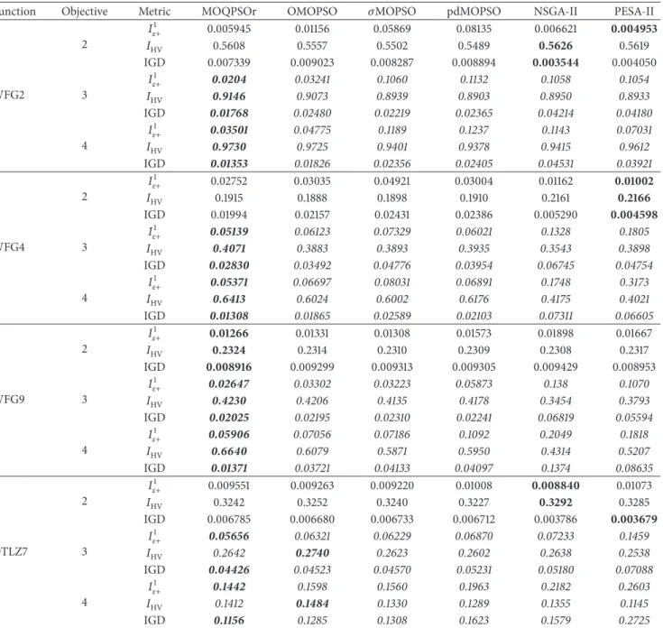
𝐼HV measures both the convergence and the diversity
of the solutions. It could be observed clearly again from Table 3 that MOQPSOr is the best-performing algorithm, yielding the best values in 7 out of 12 problems. The next best-performing algorithms are NSGA-II and PESA-II, which achieve 2 best values each. Although MOQPSOr does not
get the best𝐼HVon 3-objective DTLZ7, it is the second best
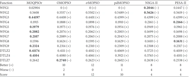
performing algorithm, only a little bit inferior to OMOPSO. Figure 4 illustrates the comparison between the final nondominated fronts obtained by MOQPSOr and those by the other algorithms on 2-objective WFG6. In order to display more clearly, each comparison pair contains an overall (Figures 4(a), 4(c), and 4(e)) figure and a sectional (Figures 4(b), 4(d), and 4(f)) figure. In each diagram in Figure 4, thin blue lines demonstrate the ideal Pareto fronts of the problems, while the red dots present the nondominated solutions obtained by MOQPSOr. The black dots in the three pairs of Figures 4(a) and 4(b), Figures 4(c) and 4(d), and Figures 4(e) and 4(f) represent the Pareto front obtained by OMOPSO, NSGA-II, and PESA-II, respectively. It could be observed from Figure 4 that, in terms of the closeness to the blue real Pareto front, NSGA-II performs the worst on 2-objective WFG6. Although the nondominated solutions obtained by OMOPSO and PESA-II are both very close to the one obtained by MOQPSOr, the latter is still a little closer to the ideal Pareto front. Besides, MOQPSOr’s nondominated solution shows a much better balanced distribution than OMOPSO’s and PESA-II’s.
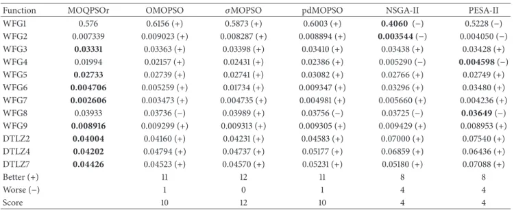
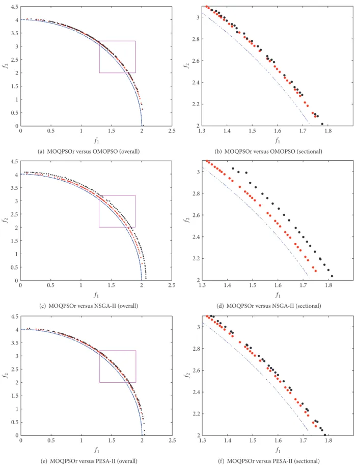
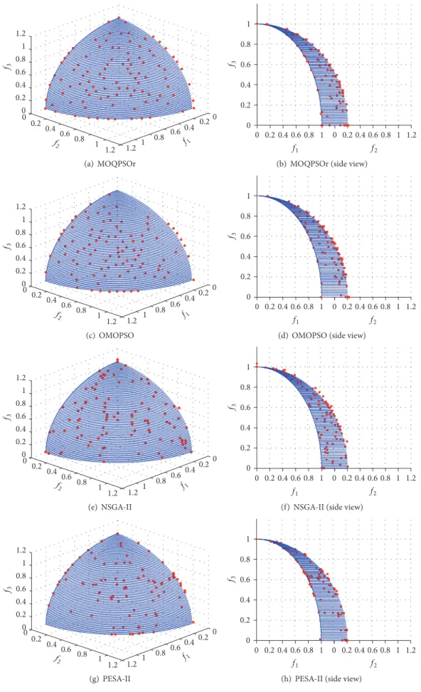
Figures 5 and 6 demonstrate the final nondominated fronts found by MOQPSOr and by other algorithms on 3-objective DTLZ2 and DTLZ7. Figures 5(a), 5(c), 5(e), 5(g),
6(a), 6(c), 6(e), and 6(g) are the overall view of the fronts; Figures 5(b), 5(d), 5(f), 6(h), 6(b), 6(d), 6(f), and 6(h) are the side views. For DTLZ2, MOQPSOr obviously achieves the best performance. It could be observed from the side views that neither NSGA-II nor PESA-II can converge to the ideal Pareto front completely, with some dots astray, the convergence of NSGA-II being even worse than PESA-II. Although the nondominated front found by OMOPSO can converge to the ideal Pareto front as MOQPSOr, its distribution is less balanced. In other words, the distribution of the nondominated front achieved by MOQPSOr is the best. It can be seen from Figure 6 that the solutions obtained by PESA-II cannot cover the entire ideal Pareto front on every plane when it runs on DTLZ7. Similar observations can also be found when NSGA-II runs on DTLZ7. In contrast, both OMOPSO and MOQPSOr can converge to the ideal Pareto front evenly.
In a word, it could be concluded that MOQPSOr is the most effective algorithm among all the 6 algorithms discussed in our study. Whether considered on solutions’ convergence or the diversity, MOQPSOr outperforms all the PSO-based algorithms here on all 12 test functions. Compared with NSGA-II and PESA-II, MOQPSOr can achieve better solu-tion sets on 8 out of 12 problems. Moreover, MOQPSOr performs the best on all the 3-objective functions.
0 0.5 1 1.5 2 2.5 0
0.5 1 1.5 2 2.5 3 3.5 4 4.5
f1
f2
(a) MOQPSOr versus OMOPSO (overall)
1.3 1.4 1.5 1.6 1.7 1.8
2 2.2 2.4 2.6 2.8 3
f1
f2
(b) MOQPSOr versus OMOPSO (sectional)
0 0.5 1 1.5 2 2.5
0 0.5 1 1.5 2 2.5 3 3.5 4 4.5
f1
f2
(c) MOQPSOr versus NSGA-II (overall)
1.3 1.4 1.5 1.6 1.7 1.8
2 2.2 2.4 2.6 2.8 3
f1
f2
(d) MOQPSOr versus NSGA-II (sectional)
0 0.5 1 1.5 2 2.5
0 0.5 1 1.5 2 2.5 3 3.5 4 4.5
f1
f2
(e) MOQPSOr versus PESA-II (overall)
1.3 1.4 1.5 1.6 1.7 1.8
2 2.2 2.4 2.6 2.8 3
f1
f2
(f) MOQPSOr versus PESA-II (sectional)
0 0.2 0.4 0.6 0.8 1 1.2 0
0.2 0.4
0.6 0.8 1 1.2 0
0.2 0.4 0.6 0.8 1 1.2
f2
f3
f1
(a) MOQPSOr
0 0.2 0.4 0.6 0.8 1 0 0.2 0.4 0.6 0.8 1 1.2 0
0.2 0.4 0.6 0.8 1
f1 f2
f3
(b) MOQPSOr (side view)
0 0.2 0.4 0.6 0.8 1 1.2 0 0.2
0.4 0.6 0.8 1
1.2 0
0.2 0.4 0.6 0.8 1 1.2
f1
f2
f3
(c) OMOPSO
0 0.2 0.4 0.6 0.8 1 0 0.2 0.4 0.6 0.8 1 1.2 0
0.2 0.4 0.6 0.8 1
f1 f2
f3
(d) OMOPSO (side view)
0 0.2 0.4 0.6 0.8 1 1.2 0 0.2
0.4 0.6 0.8 1
1.2 0
0.2 0.4 0.6 0.8 1 1.2
f1
f2
f3
(e) NSGA-II
0 0.2 0.4 0.6 0.8 1 0 0.2 0.4 0.6 0.8 1 1.2 0
0.2 0.4 0.6 0.8 1
f1 f2
f3
(f) NSGA-II (side view)
0 0.2 0.4 0.6 0.8 1 1.2 0
0.2 0.4
0.6 0.8 1 1.2 0
0.2 0.4 0.6 0.8 1 1.2
f2
f3
f1
(g) PESA-II
0 0.2 0.4 0.6 0.8 1 0 0.2 0.4 0.6 0.8 1 1.2 0
0.2 0.4 0.6 0.8 1
f1 f2
f3
(h) PESA-II (side view)
0 0.2 0.4 0.6 0.8 1 0
0.2 0.4
0.6 0.8
1 2.53
3.54 4.55 5.56
f1
f2
f3
(a) MOQPSOr
0.2 0.4 0.6 0.8
1 1 0.8 0.6 0.4 0.2 0
2.5 3 3.5 4 4.5 5 5.5 6
f1 f2
f3
(b) MOQPSOr (side view)
0 0.2 0.4 0.6 0.8 1 0
0.2 0.4
0.6 0.8
1 2.53
3.54 4.55 5.56
f1
f2
f3
(c) OMOPSO
0.2 0.4 0.6 0.8
1 1 0.8 0.6 0.4 0.2 0
2.5 3 3.5 4 4.5 5 5.5 6
f1 f2
f3
(d) OMOPSO (side view)
0 0.2 0.4 0.6 0.8 1 0
0.2 0.4
0.6 0.8
1 2.53
3.54 4.55 5.56 6.5
f1
f2
f3
(e) NSGA-II
0.2 0.4 0.6 0.8
1 1 0.8 0.6 0.4 0.2 0
2.5 3 3.5 4 4.5 5 5.5 6 6.5
f1 f2
f3
(f) NSGA-II (side view)
0 0.2 0.4 0.6 0.8 1 0
0.2 0.4
0.6 0.8
1 2.53
3.54 4.55 5.56 6.5
f1
f2
f3
(g) PESA-II
0.2 0.4 0.6 0.8
1 1 0.8 0.6 0.4 0.2 0
2.5 3 3.5 4 4.5 5 5.5 6 6.5
f1 f2
f3
(h) PESA-II (side view)
Table 5: Experiment results of all the algorithms in terms of𝐼𝜀+1,𝐼HV, and IGD on multimodal functions.
Function Objective Metric MOQPSOr OMOPSO 𝜎MOPSO pdMOPSO NSGA-II PESA-II
WFG2
2
𝐼1
𝜀+ 0.005945 0.01156 0.05869 0.08135 0.006621 0.004953
𝐼HV 0.5608 0.5557 0.5502 0.5489 0.5626 0.5619
IGD 0.007339 0.009023 0.008287 0.008894 0.003544 0.004050
3
𝐼1
𝜀+ 0.0204 0.03241 0.1060 0.1132 0.1058 0.1054
𝐼HV 0.9146 0.9073 0.8939 0.8903 0.8950 0.8933
IGD 0.01768 0.02480 0.02219 0.02365 0.04214 0.04180
4
𝐼1
𝜀+ 0.03501 0.04775 0.1189 0.1237 0.1143 0.07031
𝐼HV 0.9730 0.9725 0.9401 0.9378 0.9415 0.9612
IGD 0.01353 0.01826 0.02356 0.02405 0.04531 0.03921
WFG4
2
𝐼1
𝜀+ 0.02752 0.03035 0.04921 0.03004 0.01162 0.01002
𝐼HV 0.1915 0.1888 0.1898 0.1910 0.2161 0.2166
IGD 0.01994 0.02157 0.02431 0.02386 0.005290 0.004598
3
𝐼1
𝜀+ 0.05139 0.06123 0.07329 0.06021 0.1328 0.1805
𝐼HV 0.4071 0.3883 0.3893 0.3935 0.3543 0.3898
IGD 0.02830 0.03492 0.04776 0.03954 0.06745 0.04754
4
𝐼1
𝜀+ 0.05371 0.06697 0.08031 0.06891 0.1748 0.3173
𝐼HV 0.6413 0.6024 0.6002 0.6176 0.4175 0.4021
IGD 0.01308 0.01865 0.02589 0.02103 0.07311 0.06605
WFG9
2
𝐼1
𝜀+ 0.01266 0.01331 0.01308 0.01573 0.01898 0.01667
𝐼HV 0.2324 0.2314 0.2310 0.2309 0.2308 0.2317
IGD 0.008916 0.009299 0.009313 0.009305 0.009429 0.008953
3
𝐼1
𝜀+ 0.02647 0.03302 0.03223 0.05873 0.138 0.1070
𝐼HV 0.4230 0.4206 0.4135 0.4178 0.3454 0.3793
IGD 0.02025 0.02195 0.02310 0.02241 0.06819 0.05594
4
𝐼1
𝜀+ 0.05906 0.07056 0.07186 0.1092 0.2049 0.1818
𝐼HV 0.6640 0.6079 0.5871 0.5950 0.4314 0.5207
IGD 0.01371 0.03721 0.04133 0.04097 0.1374 0.08635
DTLZ7
2
𝐼1
𝜀+ 0.009551 0.009263 0.009220 0.01008 0.008840 0.01073
𝐼HV 0.3242 0.3252 0.3240 0.3227 0.3292 0.3285
IGD 0.006785 0.006680 0.006733 0.006712 0.003786 0.003679
3
𝐼1
𝜀+ 0.05656 0.06321 0.06229 0.06870 0.07233 0.1459
𝐼HV 0.2642 0.2740 0.2623 0.2602 0.2638 0.2538
IGD 0.04426 0.04523 0.04570 0.05231 0.05180 0.07088
4
𝐼1
𝜀+ 0.1442 0.1598 0.1560 0.1963 0.2182 0.2603
𝐼HV 0.1412 0.1484 0.1330 0.1289 0.1355 0.1145
IGD 0.1156 0.1285 0.1308 0.1623 0.1579 0.2725
algorithm on 2-objective WFG2 and WFG4, with a more obvious disadvantage especially towards NSGA-II and PESA-II, it turns out to be much more effective than all of the other algorithms when dealing with the 3-objective and 4-objective optimizations. In addition, the lead swells as the number of objectives increases. In conclusion, MOQPSOr is a competi-tive multiobjeccompeti-tive optimization algorithm, especially on the multimodal problems with large number of objectives.
5. Conclusion
Generally speaking, most multiobjective optimization algo-rithms are reformed from various single-objective optimiz-ers, and the latter play vital roles in deciding the performance
which makes the swarm mutates more than the original QPSO. With a high degree of probability, the local attractor
𝑝 is located near the personal best position during the
early stage of the search but near the global best position
gbest in the later stage of iteration. Unlike most MOPSOs,
there is no additional mutation operation in MOQPSOr. Compared with the 5 widely used evolutionary multiobjective optimization algorithms on 12 benchmark functions, the experiment results show that the proposed algorithm is highly competitive in both convergence and diversity when solving the multiobjective optimization problems. On top of that, the advantage becomes even more obvious with the number of objectives increasing.
Competing Interests
The authors have no conflict of interests regarding the publication of this manuscript.
Acknowledgments
This work was supported by the Natural Science Foun-dation of Jiangsu province (Project nos. BK20130155 and BK20130160).
References
[1] Y. Liu, F. Chen, M. Li, and J. Kou, “A multi-objective
optimiza-tion model for informaoptimiza-tion system design,” inContemporary
Research on E-Business Technology and Strategy, pp. 486–495, Springer, 2012.
[2] J. Luo, Y. Qi, J. Xie, and X. Zhang, “A hybrid multi-objective PSO-EDA algorithm for reservoir flood control operation,” Applied Soft Computing Journal, vol. 34, pp. 526–538, 2015. [3] B. Amiri, L. Hossain, J. W. Crawford, and R. T. Wigand,
“Community detection in complex networks: multi-objective
enhanced firefly algorithm,”Knowledge-Based Systems, vol. 46,
pp. 1–11, 2013.
[4] M. Fadaee and M. A. M. Radzi, “Multi-objective optimization of a stand-alone hybrid renewable energy system by using
evolutionary algorithms: a review,”Renewable and Sustainable
Energy Reviews, vol. 16, no. 5, pp. 3364–3369, 2012.
[5] J. Moore and R. Chapman, Application of Particle Swarm to
Multiobjective Optimization, Department of Computer Science and Software Engineering, Auburn University, Auburn, Ala, USA, 1999.
[6] M. R. Sierra and C. A. C. Coello, “Improving PSO-based
multi-objective optimization using crowding, mutation and
∈-dominance,” inEvolutionary Multi-Criterion Optimization, C.
A. C. Coello, A. H. Aguirre, and E. Zitzler, Eds., vol. 3410 of Lecture Notes in Computer Science, pp. 505–519, Springer, Berlin, Germany, 2005.
[7] M. R. Sierra and C. A. C. Coello, “Multi-objective particle
swarm optimizers: a survey of the state-of-the-art,”
Interna-tional Journal of ComputaInterna-tional Intelligence Research, vol. 2, pp. 287–308, 2006.
[8] A. Zhou, B.-Y. Qu, H. Li, S.-Z. Zhao, P. N. Suganthan, and Q. Zhang, “Multiobjective evolutionary algorithms: a survey of the
state of the art,”Swarm and Evolutionary Computation, vol. 1, no.
1, pp. 32–49, 2011.
[9] M. A. Abido, “Multiobjective particle swarm optimization with
nondominated local and global sets,”Natural Computing, vol. 9,
no. 3, pp. 747–766, 2010.
[10] J. Branke and S. Mostaghim, “About selecting the personal
best in multi-objective particle swarm optimization,” inParallel
Problem Solving from Nature—PPSN IX, T. P. Runarsson, H.-G. Beyer, E. Burke, J. J. Merelo-Guerv´os, L. D. Whitley, and X. Yao,
Eds., vol. 4193 ofLecture Notes in Computer Science, pp. 523–532,
Springer, Berlin, Germany, 2006.
[11] Y. Wang and Y. Yang, “Particle swarm optimization with preference order ranking for multi-objective optimization,” Information Sciences, vol. 179, no. 12, pp. 1944–1959, 2009.
[12] F. Van Den Bergh,An Analysis of Particle Swarm Optimizers,
University of Pretoria, 2006.
[13] F. J. Solis and R. J. B. Wets, “Minimization by random search
techniques,”Mathematics of Operations Research, vol. 6, no. 1,
pp. 19–30, 1981.
[14] J. Sun, B. Feng, and W. Xu, “Particle swarm optimization
with particles having quantum behavior,” inProceedings of the
Congress on Evolutionary Computation (CEC ’04), Portland, Ore, USA, June 2004.
[15] L. dos Santos Coelho and P. Alotto, “Global optimization of elec-tromagnetic devices using an exponential quantum-behaved
particle swarm optimizer,”IEEE Transactions on Magnetics, vol.
44, no. 6, pp. 1074–1077, 2008.
[16] Y. Cai, J. Sun, J. Wang et al., “Optimizing the codon usage of
synthetic gene with QPSO algorithm,” Journal of Theoretical
Biology, vol. 254, no. 1, pp. 123–127, 2008.
[17] C. Sun and S. Lu, “Short-term combined economic emission hydrothermal scheduling using improved quantum-behaved
particle swarm optimization,”Expert Systems with Applications,
vol. 37, no. 6, pp. 4232–4241, 2010.
[18] J. Sun, X. Wu, V. Palade, W. Fang, C.-H. Lai, and W. Xu, “Convergence analysis and improvements of quantum-behaved
particle swarm optimization,”Information Sciences, vol. 193, pp.
81–103, 2012.
[19] J. Sun, W. Fang, X. Wu, V. Palade, and W. Xu, “Quantum-behaved particle swarm optimization: analysis of individual
particle behavior and parameter selection,”Evolutionary
Com-putation, vol. 20, no. 3, pp. 349–393, 2012.
[20] J. D. Schaffer, “Multiple objective optimization with vector
evaluated genetic algorithms,” inProceedings of the 1st
Interna-tional Conference on Genetic Algorithms, pp. 93–100, L. Erlbaum Associates, Pittsburgh, Pa, USA, July 1985.
[21] N. Tian and Z. Ji, “Pareto-ranking based quantum-behaved particle swarm optimization for multiobjective optimization,” Mathematical Problems in Engineering, vol. 2015, Article ID 940592, 10 pages, 2015.
[22] J. Kennedy, “Particle swarm optimization,” inEncyclopedia of
Machine Learning, Springer, Berlin, Germany, 2011.
[23] J. Kennedy and R. Eberhart, “Particle swarm optimization,” in Proceedings of the IEEE International Conference on Neural Net-works, pp. 1942–1948, Perth, Australia, November-December 1995.
[24] M. Clerc and J. Kennedy, “The particle swarm-explosion, sta-bility, and convergence in a multidimensional complex space,” IEEE Transactions on Evolutionary Computation, vol. 6, no. 1, pp. 58–73, 2002.
[25] K. Deb, A. Pratap, S. Agarwal, and T. Meyarivan, “A fast
and elitist multiobjective genetic algorithm: NSGA-II,”IEEE
[26] S. Huband, P. Hingston, L. Barone, and L. While, “A review of multiobjective test problems and a scalable test problem
toolkit,”IEEE Transactions on Evolutionary Computation, vol.
10, no. 5, pp. 477–506, 2006.
[27] E. Zitzler, K. Deb, and L. Thiele, “Comparison of multiobjective
evolutionary algorithms: empirical results,”Evolutionary
Com-putation, vol. 8, no. 2, pp. 173–195, 2000.
[28] K. Deb, L. Thiele, M. Laumanns, and E. Zitzler,Scalable Test
Problems for Evolutionary Multiobjective Optimization, Springer, Berlin, Germany, 2005.
[29] E. Zitzler, L. Thiele, M. Laumanns, C. M. Fonseca, and V. G. Da Fonseca, “Performance assessment of multiobjective
optimiz-ers: an analysis and review,”IEEE Transactions on Evolutionary
Computation, vol. 7, no. 2, pp. 117–132, 2003.
[30] E. Zitzler and L. Thiele, “Multiobjective evolutionary algo-rithms: a comparative case study and the strength Pareto
approach,”IEEE Transactions on Evolutionary Computation, vol.
3, no. 4, pp. 257–271, 1999.
[31] K. Deb and H. Jain, “An evolutionary many-objective opti-mization algorithm using reference-point-based nondominated sorting approach—part I: solving problems with box
con-straints,”IEEE Transactions on Evolutionary Computation, vol.
18, no. 4, pp. 577–601, 2014.
[32] C. M. Fonseca, J. D. Knowles, L. Thiele, and E. Zitzler, “A tutorial on the performance assessment of stochastic multiobjective
optimizers,” inProceedings of the 3rd International Conference
on Evolutionary Multi-Criterion Optimization (EMO ’05), p. 240, Guanajuato, Mexico, March 2005.
[33] S. Mostaghim and J. Teich, “Strategies for finding good local guides in multi-objective particle swarm optimization
(MOPSO),” in Proceedings of the IEEE Swarm Intelligence
Symposium (SIS ’03), pp. 26–33, IEEE, Indianapolis, Ind, USA, April 2003.
[34] J. E. Alvarez-Benitez, R. M. Everson, and J. E. Fieldsend, “A MOPSO algorithm based exclusively on pareto dominance
concepts,” inProceedings of the 3rd International Conference on
Evolutionary Multi-Criterion Optimization (EMO ’05), pp. 459– 473, Springer, Guanajuato, Mexico, March 2005.
[35] D. W. Corne, N. R. Jerram, J. D. Knowles, and M. J. Oates, “PESA-II: region-based selection in evolutionary multiobjective
optimization,” inProceedings of the Genetic and Evolutionary
Computation Conference (GECCO ’01), San Francisco, Calif, USA, July 2001.
[36] J. J. Durillo, J. Garc´ıa-Nieto, A. J. Nebro, C. A. C. Coello, F. Luna, and E. Alba, “Multi-objective particle swarm optimizers:
an experimental comparison,” inEvolutionary Multi-Criterion
Optimization, M. Ehrgott, C. M. Fonseca, X. Gandibleux,
J.-K. Hao, and M. Sevaux, Eds., vol. 5467 ofLecture Notes in
Computer Science, pp. 495–509, Springer, Berlin, Germany, 2009.
Submit your manuscripts at
http://www.hindawi.com
Hindawi Publishing Corporation
http://www.hindawi.com Volume 2014
Mathematics
Journal ofHindawi Publishing Corporation
http://www.hindawi.com Volume 2014 Mathematical Problems in Engineering
Hindawi Publishing Corporation http://www.hindawi.com
Differential Equations
International Journal of
Volume 2014
Hindawi Publishing Corporation
http://www.hindawi.com Volume 2014 Hindawi Publishing Corporationhttp://www.hindawi.com Volume 2014
Hindawi Publishing Corporation
http://www.hindawi.com Volume 2014 Mathematical PhysicsAdvances in
Complex Analysis
Journal ofHindawi Publishing Corporation
http://www.hindawi.com Volume 2014
Optimization
Journal ofHindawi Publishing Corporation
http://www.hindawi.com Volume 2014
Combinatorics
Hindawi Publishing Corporation
http://www.hindawi.com Volume 2014
International Journal of
Hindawi Publishing Corporation
http://www.hindawi.com Volume 2014
Journal of
Hindawi Publishing Corporation
http://www.hindawi.com Volume 2014
Function Spaces
Abstract and Applied Analysis Hindawi Publishing Corporation
http://www.hindawi.com Volume 2014
International Journal of Mathematics and Mathematical Sciences
Hindawi Publishing Corporation http://www.hindawi.com Volume 2014
The Scientific
World Journal
Hindawi Publishing Corporationhttp://www.hindawi.com Volume 2014
Hindawi Publishing Corporation
http://www.hindawi.com Volume 2014
Discrete Dynamics in Nature and Society Hindawi Publishing Corporation
http://www.hindawi.com Volume 2014 Hindawi Publishing Corporation
http://www.hindawi.com Volume 2014
Discrete Mathematics
Journal ofHindawi Publishing Corporation
http://www.hindawi.com Volume 2014 Hindawi Publishing Corporationhttp://www.hindawi.com Volume 2014