MODEL IMPLIED INSTRUMENTAL VARIABLE ESTIMATION FOR MULTILEVEL CONFIRMATORY FACTOR ANALYSIS
Michael L. Giordano
A thesis submitted to the faculty at the University of North Carolina at Chapel Hill in partial fulfillment of the requirements for the degree of Master of Arts in Psychology and Neuroscience
in the College of Arts and Sciences.
Chapel Hill 2018
ABSTRACT
Michael L. Giordano: Model Implied Instrumental Variable Estimation for Multilevel Confirmatory Factor Analysis
(Under the direction of Kenneth Bollen)
Multilevel Confirmatory Factor Analysis (MCFA) models are most commonly estimated with full information maximum likelihood (FIML). FIML is asymptotically efficient and
asymptotically unbiased given correct model specification and no excessive multivariate kurtosis. When these assumptions are violated, we have no guarantee about the asymptotic properties of FIML. In single level SEMs, the Model Implied Instrument Variable (MIIV-2SLS) estimator has been shown to be an excellent alternative to maximum likelihood. Following prior work for single level SEMs, this paper develops two MIIV-2SLS estimators for MCFA models. I evaluate both estimators in comparison to FIML with a Monte Carlo simulation study varying number of clusters, cluster size, distribution of data, balance of clusters and correct versus incorrect model specifications. Results suggest that both MIIV estimators are good alternatives to FIML across a variety of conditions. Most importantly, they are more robust to model misspecification and offer local tests of fit with Sargan’s test. The primary limitation found in
TABLE OF CONTENTS
LIST OF TABLES ...v
LIST OF FIGURES ...vii
Introduction ...1
Chapter 1: MIIV-2SLS estimation for MCFA ...5
Multilevel Latent Variable Models ...5
MIIV-2SLS ...13
MIIV-2SLS Estimator for MCFAs ...18
Chapter 2: Simulation Study ...22
Simulation Design ...22
Results ...26
True Model, No Skew/Kurtosis, Balanced Clusters ...26
Performance under structural misspecification ...28
Performance under distributional misspecification ...31
Performance given unbalanced data ...32
Examining Sargan’s test performance ...34
Chapter 3: Conclusions ...36
APPENDIX A: TABLES ...46
APPENDIX B: FIGURES ...60
LIST OF TABLES
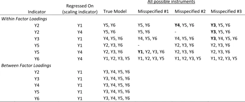
Table 1. Reviewing estimation equations and instruments for MIIV-2SLS procedures. Bolded indicators are false instruments based on the True model, but used in the corresponding condition because they are implied
by the specified model. ...46 Table 2. Number of converged FIML models by various conditions and sample
sizes, for true model specifications. ...47 Table 3. RMSE across CN/CS condition, for the true model specification. Clusters
are balanced and all data are multivariate normal. ...48 Table 4. Empirical SD of estimates vs (Mean SE) across each CN/CS for the true
model specification. All data are multivariate normal and clusters are
balanced. ...49 Table 5. RMSE across CN/CS condition, for misspecification #1 (missing L1 by
Y5 factor loading). Clusters are balanced and all data are multivariate
normal. ...50 Table 6. Empirical SD of estimates vs (Mean SE) across each CN/CS for
misspecification #1 (Missing L1 by Y5 factor loading). All data are
multivariate normal and clusters are balanced. ...51 Table 7. RMSE across CN/CS condition, for misspecification #2 (missing L2 by
Y2 factor loading). Clusters are balanced and all data are multivariate
normal. ...52 Table 8. Empirical SD of estimates vs (Mean SE) across each CN/CS for
misspecification #2 (missing L2 by Y2 factor loading). All data are
multivariate normal and clusters are balanced. ...53 Table 9. RMSE across CN/CS condition, for misspecification #3 (missing Y2 and
Y3 correlated residual). Clusters are balanced and all data are multivariate
normal. ...54 Table 10. Empirical SD of estimates vs (Mean SE) across each CN/CS for
misspecification #3 (missing Y2 and Y3 correlated residual). All data are
multivariate normal and clusters are balanced. ...55 Table 11. RMSE across various combinations of Skew/Kurtosis. Within groups
Table 12. Empirical SD of estimates vs (Mean SE) across skew/kurtosis
conditions. CN=100, CS=30. All clusters are balanced and fit with fit with
true model specification. ...57 Table 13. RMSE across CN/CS condition with unbalanced clusters. All data are
multivariate normal and fit with true model specification. ...58 Table 14. Empirical SD of estimates vs (Mean SE) across each CN/CS for
unbalanced clusters. All data are multivariate normal and fit with the true
LIST OF FIGURES
Figure 1. Population model data generating model. True model contains all solid dashed and dotted lines. Misspecification #1 omits the path between 𝐿𝑊1 and Y5. Misspecification #2 omits the path between 𝐿𝑊2 and Y2.
Misspecification #3 omits the correlated residual between Y2 and Y3. ...60 Figure 2. Relative bias boxplots for each factor loading in the True Model
condition. Black line represents median relative bias. Black dot represents mean relative bias. Colors separate different estimators and each cell is a different combination of CN and CS. All clusters are balanced and
multivariate normal. ...61 Figure 3. Relative bias boxplots for variance/covariance parameters in the True
Model condition. Black line represents median relative bias. Black dot represents mean relative bias. Colors separate different estimators and each cell is a different combination of CN and CS. All clusters are
balanced and multivariate normal. ...62 Figure 4. Relative bias boxplots for each factor loading in the Misspecified # 1
condition (missing the L1 by Y5 factor loading). Black line represents median relative bias. Black dot represents mean relative bias. Colors separate different estimators and each cell is a different combination of
CN and CS. All clusters are balanced and multivariate normal. ...63 Figure 5. Relative bias boxplots for each factor loading in the Misspecified # 2
condition (missing the L2 by Y2 factor loading). Black line represents median relative bias. Black dot represents mean relative bias. Colors separate different estimators and each cell is a different combination of
CN and CS. All clusters are balanced and multivariate normal. ...64 Figure 6. Relative bias boxplots for each factor loading in the Misspecified # 3
condition (missing the correlated residual between Y2 and Y3). Black line represents median relative bias. Black dot represents mean relative bias. Colors separate different estimators and each cell is a different
combination of CN and CS. All clusters are balanced and multivariate
normal. ...65 Figure 7. Relative bias boxplots for each factor loading across the Skew/Kurtosis
conditions. CN=100 and CS=30, while trends here generalized to other CN/CS conditions. Black line represents median relative bias. Black dot represents mean relative bias. Colors separate different estimators and each cell is a different combination skew/kurtosis condition. All clusters
mean relative bias. Colors separate different estimators and each cell is a different combination of CN and CS. All data are multivariate normal and
fit with the true model specification. ...67 Figure 9. Sargan’s test rejection rates for each factor loading in the True Model
condition. Colors separate different estimators and each cell is a different combination of CN and CS. All clusters are balanced and multivariate
normal. ...68 Figure 10. Sargan’s Test Rejection Rates for each factor loading in the
Misspecified # 1 condition (missing the L1 by Y5 factor loading). Colors separate different estimators and each cell is a different combination of
CN and CS. All clusters are balanced and multivariate normal. ...69 Figure 11. Sargan’s Test Rejection Rates for each factor loading in the
Misspecified # 2 condition (missing the L2 by Y2 factor loading). Colors separate different estimators and each cell is a different combination of
CN and CS. All clusters are balanced and multivariate normal. ...70 Figure 12. Sargan’s Test Rejection Rates for each factor loading in the
Misspecified # 3 condition (missing the correlated residual between Y2 and Y3). Colors separate different estimators and each cell is a different combination of CN and CS. All clusters are balanced and multivariate
normal. ...71 Figure 13. Sargan’s Test Rejection Rates for each factor loading across the
Skew/Kurtosis conditions. CN=100 and CS=30, while trends here generalized to other CN/CS conditions. Colors separate different estimators and each cell is a different combination skew/kurtosis condition. All clusters are balanced and data are fit with the true model
specification. ...72 Figure 14. Sargan’s Test Rejection Rates for each factor loading in the
unbalanced clusters condition. Colors separate different estimators and each cell is a different combination of CN and CS. All data are
Introduction
Multilevel confirmatory factor analysis (MCFA) has grown in popularity over the past several decades. Leveraging the strengths of multilevel modeling and confirmatory factor analysis, MCFAs allow for the simultaneous modeling of measurement error and hierarchically clustered data. In common applications, standard confirmatory factor analysis accounts for measurement error, but is not typically used to account for nested or clustered data. Standard multilevel models, on the other hand, are used for analyzing clustered data, but not typically used to simultaneously account for measurement error.1 Many studies have shown the deep
connections between multilevel models and latent variable models, often illustrating equivalence between the methods (Bauer, 2003; Curran, 2003; Kamata, Bauer, & Miyazaki, 2008; Mehta & Neale, 2005; Meredith & Tisak, 1990).
Given the overlap between latent variable models and MLM, modern research in
psychometrics has sought to unify latent variable models with multilevel models (Asparouhov & Muthén, 2003; Rabe-Hesketh, Skrondal, & Pickles, 2004; Rabe-Hesketh, Skrondal, & Zheng, 2007). The developments in MCFAs have led to approaches for modeling clustered data with measurement error and heterogeneous factor structures at the within and between levels (Asparouhov & Muthén, 2003, 2007; Bentler & Liang, 2003; Goldstein, 1987; Goldstein & McDonald, 1988; Kim, Dedrick, Cao, & Ferron, 2016; Longford & Muthén, 1992; McDonald, 1994; McDonald & Goldstein, 1989; Muthén, 1989, 1990, 1994, Rabe-Hesketh et al., 2004,
1
2007, p. 207; Skrondal & Rabe-Hesketh, 2004). Of course, latent variable models are diverse. Modern multilevel latent variable models could include multilevel IRT, multilevel factor analysis, and multilevel structural equation modeling. For this study I will focus on multilevel factor analysis specifically, but it is my hope that future work could expand on this to include more general multilevel structural equation models.
First, it is important to establish why MCFA is needed. One of the assumptions made in CFA (or SEM more broadly), is that observations are independent and identically distributed. When data are clustered we violate this assumption. Given clustered measurement data, we might be tempted to ignore clustering, especially if we are not interested in all levels in the measurement model. However, this would be naïve. Julian (2001) showed that ignoring
clustering in CFA results in biased loadings, unique variances, factor variances. In the more full SEM context, du Toit & Toit (2008) showed that ignoring clustering resulted in incorrect
parameter estimates, standard errors and inappropriate fit statistics. In short, if data are clustered then researchers need to consider multilevel analyses (or other corrections).
one of the more unique features of MCFAs, which is the option to model different factor structures for within-groups and between-groups.
Given the relative complexity of these models, MCFA estimation is an area of ongoing methodological development. Before general maximum likelihood methods were available, early estimation approaches relied on decomposing variance-covariance matrices at different levels and fitting factor models with traditional SEM software, using the variance covariance matrices in place of raw data. These early methods have been called pseudo-maximum likelihood methods or ‘ad-hoc’ methods (Goldstein, 1987; McDonald & Goldstein, 1989; Muthén & Satorra, 1989).
Today, full information maximum likelihood (FIML) estimation routines are available through Mplus, Stata’s GLLAMM routine, the ‘OpenMx’ package in R, and the ‘xxM’ package in R (Asparouhov & Muthén, 2003; Mehta, 2013; Muthén & Muthén, 2015; Neale et al., 2016; Rabe-Hesketh et al., 2004; StataCorp, 2015) 2.
Unsurprisingly, FIML estimation has become the de facto estimation method in most applications. Maximum likelihood offers the usual properties of being asymptotically efficient and asymptotically unbiased—excellent qualities to have. However, these properties require strong assumptions such as correct model specification and no excessive multivariate kurtosis. If these assumptions are violated, there is no guarantee about the asymptotic efficiency or
convergence would also be a potential barrier in MCFA (Preacher, Zhang, & Zyphur, 2015; Preacher, Zyphur, & Zhang, 2010; Ryu & West, 2009).
Given the potential shortcomings of FIML for MCFA, I am proposing to look to the class of Two-Stage Least Squares (2SLS) instrumental variable estimators which have been shown to be effective estimators in single-level SEMs (Bollen, 2001; Bollen, Kirby, Curran, Paxton, & Chen, 2007). Bollen (1996b) proposed the Model Implied Instrumental Variable Two-Stage Least Squares (MIIV-2SLS) estimator for single level SEM’s. Under ideal conditions for ML, simulation studies found similar efficiency for MIIV estimators. It is more robust to model misspecification, it requires fewer distributional assumptions and it is computationally efficient. Also because it is non-iterative it is not subject to non-convergence issues. For these reasons, I believe that the MIIV-2SLS can be a useful estimator in MSEM’s.
Chapter 1: MIIV-2SLS estimation for MCFA Multilevel Latent Variable Models
The earliest work on multilevel latent variable models was in an unpublished dissertation by Schmidt (1969). Schmidt studied multivariate random effects and provided a computer program for maximum likelihood estimation—though this early work did not consider group level structures or variables, instead focusing on what I will call the ‘within groups’ model. Most MSEM applications specify separate within-groups and between-group structures and Schmidt’s dissertation did not deal with separate between and within components. Instead it dealt with a special case where the between and within components were equivalent. Aside from this very early work on multilevel models with latent variables, McDonald, Goldstein, Muthén, Rabe-Hesketh have been very active pushing forward the methodology for these models (Goldstein, 1987; Goldstein & McDonald, 1988; McDonald & Goldstein, 1989; Muthén, 1990; Rabe-Hesketh et al., 2007). See Hox (2010) for an excellent overview of both early and more modern approaches. I will review some of the notable techniques, focusing on the measurement model.
The particular multilevel factor analysis model that I will examine is the random intercepts MCFA. The expression for the random intercepts MCFA model is given by:
𝒀𝒊𝒋= 𝒀𝑾𝒊𝒋+ 𝒀𝑩𝒋
𝒀𝒊𝒋= 𝜶 + (𝚲𝑾𝑳𝑾𝒊𝒋+ 𝜺𝑾𝒊𝒋) + (𝚲𝑩𝑳𝑩𝒋+ 𝜺𝑩𝒋) (1)
𝑳𝑩𝒋~𝑵(𝟎, 𝜱𝑩)
𝑳𝑾𝒊𝒋~𝑵(𝟎, 𝜱𝑾)
𝜺𝑩𝒋~𝑵(𝟎, 𝜣𝑩)
𝜺𝑾𝒊𝒋~𝑵(𝟎, 𝜣𝑾)
(2)
In this model 𝛼 is a vector of measurement intercepts, 𝚲𝑾 is a vector of within groups factor loadings, 𝑳𝑾𝒊𝒋 is the vector of within groups latent variables, 𝚲𝑩 is a vector of between groups
factor loadings, 𝑳𝑩𝒋 is the vector of between groups latent variables, and 𝜺𝑾𝒊𝒋/𝜺𝑩𝒋 are vectors of
within and between residuals. We can derive the model implied covariance matrix as
𝐶𝑜𝑣(𝒀𝒊𝒋) = 𝐶𝑜𝑣 (𝒀𝒃𝒋+ 𝒀𝒘𝒊𝒋)
= 𝐶𝑜𝑣 (𝒀𝒃𝒋) + 𝐶𝑜𝑣 (𝒀𝒘𝒊𝒋)
= 𝜮𝑩+ 𝜮𝑾
= 𝜦𝑩𝜱𝑩𝜦𝑩′ + 𝜣𝑩+ 𝜦𝑾𝜱𝑾𝜦𝑾′ + 𝜣𝑾
(3)
where 𝐶𝑜𝑣 (𝒀𝒃𝒋 + 𝒀𝒘𝒊𝒋) = 𝐶𝑜𝑣 (𝒀𝒃𝒋) + 𝐶𝑜𝑣 (𝒀𝒘𝒊𝒋) based on the assumption that the within
and between models are orthogonal.
As I have already mentioned the most ubiquitous method for estimating MSEMs is FIML. Muthén (1990) derived the ML fitting function as
FML = ∑(𝒏𝒋− 𝟏){𝐥𝐨𝐠|𝚺𝑾(𝜽)| + 𝒕𝒓(𝚺𝑾−𝟏(𝜽)𝑺𝒚𝑾𝒋)} + 𝑱
𝒋=𝟏
∑𝐉𝐣=𝟏{𝐥𝐨𝐠|𝚺𝐠𝐣(𝛉)| + 𝐭𝐫(𝚺𝐠𝐣−𝟏(𝛉)𝐒𝐠𝐣)}
(4)
multivariate kurtosis). If these qualities do not hold then we have no guarantee about the asymptotic properties of our estimator.
FIML estimation is also available via the generalized linear latent and mixed models (GLLAMM) approach developed by Skrondal & Rabe-Hesketh (2004). This modeling approach can be used to estimate multilevel latent variable models with full maximum likelihood. The FIML solution available in the Mplus uses a structural equation modeling approach, while the GLLAMM framework is more akin to traditional multilevel models setup. GLLAMM has some nice properties in that it can handle a larger number of levels, missing data, unbalanced designs and flexible factor structures (FIML can handle many of these as well). As with other ML approaches GLLAMM relies on correct model specification and distributional assumptions for significance tests. Additionally, MSEM models tend to take a long time to estimate in
GLLAMM, limiting their practicality.
The idea of decomposing variances into different levels is nothing new (Cornfield & Tukey, 1956; Searle, Casella, & McCulloch, 1992). We can imagine decomposing an individual observed variable into parts as,
𝑌𝑖𝑗 = 𝑌𝑖𝑗𝑊+ 𝑌𝑖𝑗𝐵 (5)
Where 𝑌𝑖𝑗𝑊is varying at the individual level and 𝑌𝑖𝑗𝐵is varying at the group level. In other words
we can decompose variation in observed variables into their group means and group mean deviations. Another way of showing this is
𝑌𝑖𝑗 = (𝑌𝑖𝑗− 𝑌̅.𝑗) + 𝑌̅.𝑗 (6)
where (𝑌𝑖𝑗 − 𝑌̅.𝑗) is group mean centered and 𝑌̅.𝑗 represents group means. Importantly, Searle,
Casella, & McCulloch (1992) showed these components are additive and orthogonal.
Similar to the single observed variable example above, early MSEM approaches relied on separating the population covariance matrices into their within-groups and between-groups components.
𝚺𝑻 = 𝚺𝑾+ 𝚺𝑩3 (7)
where 𝚺𝑻 is the total covariance, 𝚺𝑾 is the within-groups covariance matrix, and 𝚺𝑩is the
between-groups covariance matrix. This was shown in Equation 3, where we separated the covariances into their constituent parts based on the assumption of orthogonality. Goldstein’s approach and Muthén’s approach differ in how they decompose the covariance components.
Goldstein (1987, 1995) proposed using a three-level multilevel model to decompose the within-groups and between-groups covariance. The general two-step procedure is (1) estimate within-groups and between-groups covariance matrices via a univariate multilevel model and
then (2) estimate MSEM with covariance matrices using ML and standard SEM software. Hox & Maas (2004) provide a nice description for fitting these models.
As an example of the Goldstein procedure, consider a simple MCFA model with three observed indicators. To obtain estimates of the within-groups and between-groups covariance matrices we specify a three-level univariate multilevel model, which I describe in more detail below. Thinking about this model hierarchically, level-1 could represent indicators, level-2 could represent individuals, and level-3 represents clusters of individuals. Alternatively, this could be a longitudinal study with indicators nested within individuals nested within time. The level-1 model is given by,
𝑌ℎ𝑖𝑗 = 𝜋1𝑖𝑗𝐷1𝑖𝑗+ 𝜋2𝑖𝑗𝐷2𝑖𝑗 + π3ij𝐷3𝑖𝑗 (8)
where D are dummy codes for indicators, h indexes indicators, i indexes individuals, and j indexes clusters. Also, note that we have removed the intercept from the model, in order to estimate the random component of each indicator instead of having one as a reference.
Additionally, we are not estimating a level-1 error term and instead this is being fixed at zero. 4 Moving up to the second level, the individual level, we re-define all 𝜋𝑝𝑖𝑗 terms allowing them to randomly vary across individuals. Level-2 equations are then,
𝜋1𝑖𝑗 = β1j+ 𝑢1𝑖𝑗 𝜋2𝑖𝑗 = β2j+ 𝑢2𝑖𝑗 𝜋3𝑖𝑗 = β3j+ 𝑢3𝑖𝑗
(9)
where βpj is the average of item p varying over clusters j and 𝑢𝑝𝑖𝑗 captures the random variation
in item p across individuals within clusters. Moving up again we redefine all 𝛽𝑝𝑗 terms at level-3
as,
𝛽1𝑗 = 𝛾1+ 𝑢1𝑗 𝛽2𝑗 = 𝛾2+ 𝑢2𝑗 𝛽3𝑗 = 𝛾3+ 𝑢3𝑗
(10)
where 𝛾𝑝 is the grand mean for item p and 𝑢𝑝𝑗 captures the random variation in item p across
clusters. Applying simple substitution we combine all three levels obtaining the reduced form equation as,
𝑌ℎ𝑖𝑗 = 𝛾1𝐷1 + 𝛾2𝐷2+ 𝛾3𝐷3+ 𝑢1𝑖𝑗𝐷1+ 𝑢2𝑖𝑗𝐷2+ 𝑢3𝑖𝑗𝐷3 + 𝑢1𝑗𝐷1+ 𝑢2𝑗𝐷2
+ 𝑢3𝑗𝐷3
(11)
Importantly, we assume that the level-2 random effects are distributed as
[ 𝑢1𝑖𝑗 𝑢2𝑖𝑗
𝑢3𝑖𝑗] ~𝐍(𝟎, 𝚺𝑾) (12)
where,
𝚺𝑾 = [
𝑽𝒂𝒓(𝒖𝟏𝒊𝒋) 𝑪𝒐𝒗(𝒖𝟐𝒊𝒋, 𝒖𝟏𝒊𝒋) 𝑪𝒐𝒗(𝒖𝟑𝒊𝒋, 𝒖𝟏𝒊𝒋) 𝑪𝒐𝒗(𝒖𝟐𝒊𝒋, 𝒖𝟏𝒊𝒋) 𝑽𝒂𝒓(𝒖𝟐𝒊𝒋) 𝑪𝒐𝒗(𝒖𝟑𝒊𝒋, 𝒖𝟐𝒊𝒋) 𝑪𝒐𝒗(𝒖𝟑𝒊𝒋, 𝒖𝟏𝒊𝒋) 𝑪𝒐𝒗(𝒖𝟑𝒊𝒋, 𝒖𝟐𝒊𝒋) 𝑽𝒂𝒓(𝒖𝟑𝒊𝒋)
] (13)
Similarly, we assume that the level-3 random effects are distributed as,
[ 𝑢1𝑗 𝑢2𝑗
𝑢3𝑗] ~𝐍(𝟎, 𝚺𝑩) (14)
where,
𝚺𝑩 = [
𝑽𝒂𝒓(𝒖𝟏𝒋) 𝑪𝒐𝒗(𝒖𝟐𝒋, 𝒖𝟏𝒋) 𝑪𝒐𝒗(𝒖𝟑𝒋, 𝒖𝟏𝒋) 𝑪𝒐𝒗(𝒖𝟐𝒋, 𝒖𝟏𝒋) 𝑽𝒂𝒓(𝒖𝟐𝒋) 𝑪𝒐𝒗(𝒖𝟑𝒋, 𝒖𝟐𝒋) 𝑪𝒐𝒗(𝒖𝟑𝒋, 𝒖𝟏𝒋) 𝑪𝒐𝒗(𝒖𝟑𝒋, 𝒖𝟐𝒋) 𝑽𝒂𝒓(𝒖𝟑𝒋)
In summary, as a part of this model we estimate the mean responses for each indicator (given by 𝛾𝑝’s) and the estimated variances and covariances of the random effects. Here we are mostly
interested in the variances and covariances of random effects. These variances and covariances are direct estimates of within group covariances, 𝚺𝑾, and the between group covariances, 𝚺𝑩,
which are used in the second step. With estimates of the within-groups and between-groups variance-covariance matrices, step 2 of the Goldstein approach is to fit within-groups and between-groups structural model using ML and 𝚺𝑾 and 𝚺𝑩 as data.
Here we have the additional choice of using ML or REML to estimate the multilevel models. In general, REML produces less biased estimates of the random components, especially at smaller sample sizes (Snijders & Bosker, 1999). ML has a tendency to negatively bias random components, though this bias shrinks as number of clusters approach infinity. ML also has a smaller MSE when considering variance components. Thus, there is a definite trade-off between bias and variance when considering estimation of the variance components.
may be difficult to scale up to more levels. Three-level multilevel models with several random effects is already computationally difficult to estimate. As more levels and more indicators are added this approach could become computationally intractable fairly quickly.5
Muthén, (1989, 1990) proposed another two-step solution to estimate MSEMs; Muthén’s method is often referred to as the pseudo-balanced or MUML (Muthén’s ML) approach
(McDonald, 1994; Muthén, 1994). He showed an unbiased estimate of 𝚺𝑾, can be computed
from the pooled within group covariance matrix
𝑺𝒑𝒘 = ∑ ∑ (𝒀𝒊𝒋− 𝒀̅𝒋)(𝒀𝒊𝒋− 𝒀̅𝒋)′ 𝑛
𝑖 𝐺 𝑗
𝑁 − 𝐺 (16)
and the between group covariance matrices can be estimated by
𝑺𝑩 =∑ 𝑛 (𝒀̅ − 𝒀̅𝒋)(𝒀̅ − 𝒀̅𝒋)′ 𝐺
𝑗
𝐺 − 1 (17)
Muthén showed that 𝑺𝒑𝒘 is an asymptotic unbiased estimator of 𝚺𝑾 and 𝑺𝑩 is an asymptotic unbiased estimator of 𝚺𝑩 assuming groups have equal sizes.
Once the variance has been decomposed, the two covariance matrices are used in multiple group model with ML as the estimator. Muthén (1990) showed how these two
covariance matrices could be modeled with existing SEM software. This technique relies partly on having balanced group sizes. Accounting for unbalanced groups in this setup is burdensome, and Muthén even proposed ignoring unbalance and using the average group size when data are not balanced (1989, 1990). Several studies have confirmed that the within portion of the model is consistently estimated using the pooled within covariance matrix and this holds across many conditions including balanced and unbalanced group sizes (Hox & Maas, 2001; Hox, Maas, &
5 With more levels and more random components, moving into a Bayesian framework is likely to make these
Brinkhuis, 2010; Yuan & Hayashi, 2005). For the between part of the model, residual variances tend to be underestimated and standard errors too small leading to alpha levels of close to 8%, instead of the expected 5%. In addition unbalanced groups do not lead to biased coefficients but they do lead to underestimated standard errors (Hox & Maas, 2001).
Each method—FIML, the Goldstein approach, and MUML—has advantages and disadvantages. While FIML is the gold standard at the moment I will pull from the Goldstein approach and the MUML approach to develop a MIIV-2SLS estimator for MCFAs. In order to do that I will first review MIIV-2SLS.
MIIV-2SLS
of 2SLS estimators were applied to the measurement model only and assumed no correlated errors. One exception was Jöreskog & Sörbom (1993) who applied Hägglund’s method to estimate the measurement model and generated the covariance matrix of latent variables. They then estimated the latent variable model by using the covariance matrices as input for a 2SLS procedure. This method still assumed no correlated errors and did not provide significance tests.
Bollen (1996b, 1996a) proposed the MIIV-2SLS estimator which is another instrumental variable estimator for latent variable models and part of the 2SLS family of estimators, though it differs from earlier ones. In contrast to earlier 2SLS methods for latent variable models, Bollen (1996b) showed how the MIIV-2SLS estimator could be applied to estimate full SEM’s with latent variables in an equation by equation basis, while also deriving standard errors and
significance tests. Bollen (2001) further developed MIIV-2SLS noting that there is a closed form to estimate the full model simultaneously instead of equation by equation. This form provides identical point estimates and standard errors. Further, Bollen (2001) provides general analytic condition for when MIIV-2SLS is robust to misspecification.
The MIIV-2SLS estimator differs from traditional instrumental variable techniques in several important ways. Early versions of a 2SLS estimator for SEM’s with latent variables, did not allow for correlated errors of measurement; the MIIV-2SLS estimator does allow correlated errors. Jöreskog and Sörbom’s versions of the 2SLS estimator required estimating the
measurement model and then estimating the latent variable model; the MIIV-2SLS estimator does not require this. Finally, MIIV-2SLS offers asymptotic standard errors for all coefficients in the model which previous versions did not.
compared bias and efficiency of ML and MIIV-2SLS in conditions of correct model specification and incorrect model specification; they concluded that in correct model
specification, results are similar and given misspecification MIIV-2SLS performed better. Cragg (1968) noted the same quality for 2SLS for simultaneous equations as compared to FIML. Bollen (1996b) developed an algorithm to automatically select model-implied instruments; Bollen & Bauer, (2004) later programmed this is SAS and Bauldry, (2014) programmed a similar procedure for general use in Stata, both of which made the process of using MIIV-2SLS more accessible. Bollen & Maydeu-Olivares, (2007) developed a polychoric instrumental variable estimator which can be used for models with categorical indicators. Bollen (1996b), proposed the use of Sargan’s test with MIIV-2SLS and Kirby & Bollen (2009) further developed their use and evaluated their performance for systematically investigating model misspecification. Bollen et al. (2014) developed generalized method of moments MIIV estimator (MIIV-GMM). Finally, Nestler (2014a, 2014b) explored estimating growth models with MIIV-2SLS.
Though I have mentioned several of the beneficial qualities of MIIV-2SLS I think it is worth briefly revisiting each again. The MIIV-2SLS estimator is distribution free, that is, the asymptotic standard errors can be used in significance testing even when observed variables are non-normal or have excessive multivariate kurtosis (Bollen, 1996b). As comparison,
Full-information maximum likelihood requires the assumptions of normality or no excessive kurtosis, though there are corrections for nonnormality (ex., Satorra & Bentler, 1994). MIIV-2SLS
model is misspecified, this information might influence estimates throughout, and can spread bias. MIIV-2SLS might have bias in any given misspecified equation, but that bias is more isolated and is less likely to spread to other parts of the model. Finally, though this has not been discussed at length in the literature, it should be noted that MIIV-2SLS is computationally efficient. It does not require an iterative procedure and instead has a closed form solution. As models become more complex this property may prove more and more advantageous.
Although the MIIV-2SLS estimator has been around for over two decades now, its general use is not widespread. This is likely due to the fact that it has not been readily available in software, until very recently. Fisher, Bollen, Gates, & Rönkkö (2016) have programmed MIIV-2SLS estimation into the “MIIVsem” package in R. Given that its use is not familiar practice to all, I will provide a simple example of estimating a single level CFA model with MIIV-2SLS. Additionally, this will further facilitate the development of the MIIV-2SLS estimator for MSEMs.
Suppose we have a simple two dimensional confirmatory factor analysis with eight observed indicators and two latent variables. The general latent variable model is given by
𝒀𝒊= 𝜶 + 𝚲𝑳𝒊+ 𝜺𝒊 (18)
And with the full matrices given by
[ 𝑌1 𝑌2 𝑌3 𝑌4 𝑌5 𝑌6 𝑌7 𝑌8]
= [ 𝛼1 𝛼2 𝛼3 𝛼4 𝛼5 𝛼6 𝛼7 𝛼8]
+
[
Λ11 0
Λ21 0
Λ31 0
Λ41 0
0 Λ52
0 Λ62
0 Λ72
0 Λ82] [𝐿1
𝐿2] +
[ 𝜀1 𝜀2 𝜀3 𝜀4 𝜀5 𝜀6 𝜀7 𝜀8]
(19)
𝐿1 is measured by 𝑌1− 𝑌4 and 𝐿2 is measured by 𝑌5− 𝑌8. In order to identify the model and
estimator to this model we will go through two steps. (1) Is to transform the model equations from latent variable equations to observed variable equations. And (2) is to identify MIIV’s and
perform instrumental variable regression.
To re-express the model equations as observed variable equations, we algebraically manipulate the scaling indicators.
𝑌1 = 𝐿1+ 𝜀1
𝐿1 = 𝑌1− 𝜀1
(20)
And we perform a similar transformation with 𝐿2 and𝑌5. With the latent variables expressed as observed variables, we simply substitute in the observed variable expression for every 𝐿1 and 𝐿2. For 𝑌2 we start with
𝑌2 = 𝛼2+ Λ21𝐿1+ 𝜀2 (21)
And after substituting the observed variable expression of 𝐿1, we have
𝑌2 = 𝛼2 + Λ21(𝑌1− 𝜀1) + 𝜀2 (22)
Finally, to simplify the expression we distribute Λ21 and create a composite error term to get
𝑌2 = 𝛼2 + Λ21𝑌1+ 𝑢1 (23)
which is an observed variable equation which suggests a simple regression model. However, we cannot use OLS regression because we would violate the typical assumption that the explanatory variables are uncorrelated with the composite error. Instead we can use instrumental variable regression to estimate the equation.
CFA and SEM it is worth noting that instruments vary from one equation to the next. Identifying MIIV’s is an important step in this procedure and as it has been mentioned there have been
several developments for automating the task in a variety of statistical software environments (Bauldry, 2014; Bollen & Bauer, 2004; Fisher et al., 2016). Once we have identified our MIIV’s we perform instrumental variable regression, equation by equation. For the 𝑌2 equation, we determine that 𝑌3− 𝑌8 are possible instruments. We regress 𝑌1 onto instruments to form 𝑌̂1.
Finally, we regress 𝑌2on 𝑌̂1to obtain estimates of 𝛼2 and Λ21. The same steps can be performed with all equations in the model.
While the two-step process is a useful way to think of performing MIIV-2SLS, it can also be done in a one-step procedure using the following expression
𝑨̂ = (𝒁̂ ′ 𝒁̂)−𝟏𝒁̂ ′ 𝒀 (24)
where
𝒁̂ = 𝑽(𝑽′𝑽)−𝟏𝑽′𝒁 (25)
And 𝒁 is a block diagonal matrix of indicators, 𝑽 is a block diagonal matrix of instrumental variables corresponding to various model equations. The derivations of this single equation form are developed and explained more fully in (Bollen, 2001).
MIIV-2SLS Estimator for MCFAs
MIIV-2SLS is applied in the second step in place of ML. Using the Goldstein approach and the MUML approach as two different starting points, I have two possible MIIV-2SLS estimators. I should note that here is that we will be using covariance matrices to fit MIIV-2SLS. Fox (1979) describes 2SLS estimation using only covariance matrices and those results can be adopted for this application; all of the general principles of MIIV-2SLS discussed prior still apply.
For the first possible estimator I will combine the Goldstein approach with MIIV-2SLS. From here I will refer to this as Goldstein-MIIV. First, estimate within-groups and between-groups variance covariance matrices with a three level multilevel model as we did in Equation (11). Second, apply MIIV-2SLS to the within-groups and between- groups covariance matrices separately to estimate the within and between portions of the MSEM. Based on prior research I might expect Goldstein to be better in cases of unbalance. On the other hand, using a parametric model in the first step requires additional distributional assumptions so Goldstein-MIIV might not perform as well given non-normality.
The second possible approach would be to combine the MUML estimator with MIIV-2SLS for another hybrid approach. I will refer to this estimator as MUML-MIIV. The first step would be to decompose the variance into the between and within levels as given in the MUML estimator in Equations (16) and (17). And again once the variance has been decomposed perform MIIV-2SLS on the covariance matrices separately. MUML-MIIV will be more computationally efficient and likely will perform less well given unbalanced clusters. Additionally it makes fewer distributional assumptions so we might expect it to be less affected given non-normality.
variances. Further, I expect that MIIV-2SLS in this case will be more robust to model
misspecification than FIML. By using MIIV-2SLS we will have access to Sargan’s tests of over-identification which is has been shown to be useful for pinpointing model misspecification on an equation by equation basis in single level SEMs. That said, I would like to add a note of caution that Sargan’s test was derived in the context of single level analyses. It has not been used in a
case like mine where the between and within covariance matrices are estimated separately. It remains to be proven whether the assumptions of Sargan’s test hold in these conditions. Finally,
MUML-MIIV should be more computationally efficient than other approaches and require fewer distributional assumptions.
The proposed approaches are not without complication either. Standard errors of our model coefficients might not reflect the normal 0.05 alpha levels. As mentioned previously simulations with the MUML estimator found the nominal alpha levels for the between-groups model was 0.08 instead of the expected .05. While one of the proposed advantages are the fewer distributional assumptions, this may be less applicable to the Goldstein approach because this model starts with the 3-level multilevel which requires distributional assumptions in order to be estimated. This 3-level multilevel model may be burdensome to estimate as well, given the number of random coefficients.
covariance parameters are estimates and we do not know whether they have similar or different sampling properties. In other words, no corrections are applied for the analysis being done on the decomposed covariance matrices in contrast to the usual single level covariance matrices upon which the test statistic is based. WE suspect that this has the potential to lead to problems with standard errors though it should not bias point estimates.
In sum, I have attempted to make the case that although ML has excellent properties it requires strong assumptions which are often unmet. Given this I developed two possible MIIV-2SLS style estimators, each with their own potential strengths and weaknesses. Next I evaluate the performance of both estimators with a Monte Carlo simulation study varying several factors that I describe in the next section. As a part of this simulation study, I had three primary
hypotheses:
1. Given a correctly specified model, balanced clusters, and multivariate normality, Goldstein-MIIV and MUML-MIIV would perform similarly to FIML with a possible slight loss of efficiency.
2. Given structural misspecification, Goldstein-MIIV and MUML-MIIV would be more robust to bias than FIML.
Chapter 2: Simulation Study Simulation Design
Data were simulated based on the population model given in Equation 1. Figure 1 shows the model via path diagram. Population values are given as:
𝚲𝑾=
[
1.0 0
0.8 0.3
0.7 0
0.0 1.0 0.3 0.8
0 0.7]
𝚲𝑩 =
[ 1.0 0.7 0.6 0.8 0.7 0.8]
𝚽𝑾 = [2.0 0.3
0.3 2.0] 𝚽𝑩 = [0.5]
𝚯𝑾=
[
0.8 0 0 0 0 0
0 0.8 0.3 0 0 0
0 0.3 0.8 0 0 0
0 0 0 0.8 0 0
0 0 0 0 0.8 0
0 0 0 0 0 0.8]
𝚯𝑩 =
[
0.2 0 0 0 0 0
0 0.2 0 0 0 0
0 0 0.2 0 0 0
0 0 0 0.2 0 0
0 0 0 0 0.2 0
0 0 0 0 0 0.2]
CN, though in practice applications are likely to encounter smaller CS and CN. I revisit cluster and sample size in my discussion.
In addition to CS and CN, I varied the balance of clusters and the underlying data distribution. Both of these factors were chosen to differentiate possible weaknesses of MUML-MIIV and Goldstein-MUML-MIIV respectively. Previous single level MCFA studies suggested that unbalanced clusters led to underestimated SE’s with MUML (Hox & Maas, 2001). In this study ‘unbalanced’ data were generated such that cluster sizes were equal to the average cluster size
plus or minus 15. For example, when CS=100 the smaller cluster size was n=85 and the larger sample size was n=115. A more severe disparity in size happens when CS=30 because the smaller cluster size n=15 and the larger cluster size n=45.
Varying the data distribution was expected to have the most impact on the Goldstein-MIIV estimator and FIML estimation. Here we have the added complication that data at both levels can stray from multivariate normality. I used four different conditions: (i) multivariate normal at the within and between level (W-MVN; B-MVN), (ii) Within Level: Skew=2,
In addition to between cell conditions I examined two within cell conditions: model specification and estimator. I fit each dataset with four different model specifications, namely the true model and 3 separate misspecified models, each missing a single model parameter. Dotted or Dashed lines in Figure 1 represent each of the 3 misspecified paths (while the true model contains all solid, dotted and dashed lines). The first misspecification was missing the cross loading 𝐿𝑊1𝑏𝑦 𝑌5. The second misspecification was missing 𝐿𝑊2𝑏𝑦 𝑌2, and the third
misspecification was missing the correlated errors between Y2 and Y3.
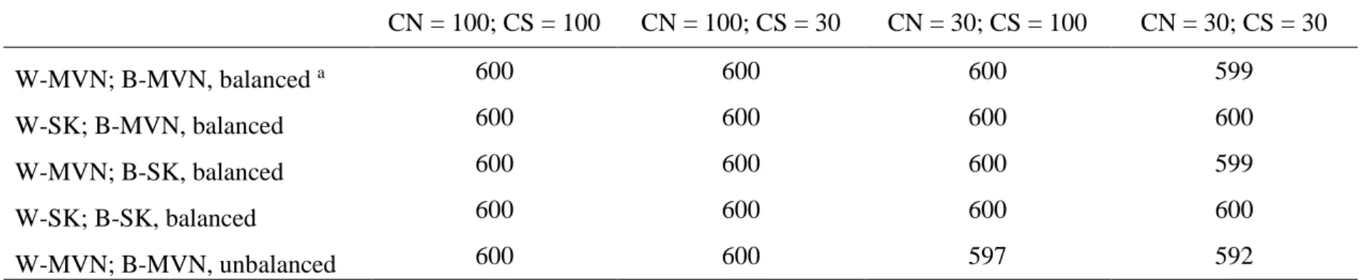
Conditions were not fully crossed, and I will briefly describe the exact combinations of factors examined6. The first set of results pertain to ideal conditions and model misspecification. I generated data from the 4 cells corresponding to all combinations of CN/CS holding clusters balanced and assuming multivariate normality (i.e., isolating the effects of sample size and model specification). I generated 600 data sets for each cell, and then fit each data set with all combinations of model specification and model estimators (2400 unique datasets and 28,000 unique models). Next I examined the effects of skew and kurtosis by generating all data for the 16 cells corresponding to all combinations of CN/CS/Skew/Kurtosis holding clusters balanced. Again I generated 600 data sets for each cell and this time fit each with all three estimators and only the true model specification (9600 unique datasets and 28,800 unique models). Finally, I examined the effects of unbalanced data by generating data from the 4 cells corresponding to all combinations of CN/CS, with unbalanced clusters assuming multivariate normality. I generated 600 datasets for each cell and fit each with all three estimators and only the true model
specification (2400 unique datasets and 7200 unique models).
6 In reality, I did run this simulation fully crossed. That’s 384 experimental conditions, 19200 independent datasets
Data were generated such that intraclass correlations were kept around 0.1 and 0.15. Hox et al. (2010) found no effect of this in a similar MSEM simulation and Preacher et al., (2010) have suggested that ICC’s lower than .05 are likely to cause convergence problems. All data
were generated in R. Multivariate normal data was generated using the ‘mvrnorm’ function from the ‘MASS’ package and non-normal data were generated using the ‘mvrnonnorm’ function from the ‘semTools’ package (Jorgensen, 2016; Venables & Ripley, 2002). FIML models were
fit in Mplus with the ‘MLR’ estimator (robust maximum likelihood, which is the default in Mplus for any multilevel procedure). MUML-MIIV and Goldstein-MIIV estimators were fit in R with self-programmed covariance decomposition functions in conjunction with the ‘MIIVsem’ package (Fisher, Bollen, Gates, & Rönkkö, 2016). Goldstein-MIIV decompositions were estimated with REML.
There is one final important note about how instrumental variables were selected for the MIIV procedures. Table 1 shows each indicator and all possible MIIVs across true and
misspecified conditions. For within group’s factor loading I used all MIIVs for each equation (varying over true and misspecified conditions). For any given equation there were between one and four instruments. For the between level factor loadings, two instruments were randomly selected (different for every iteration) from the list of all possible MIIV’s. Previous studies have
shown that using too many instruments with small sample sizes can lead to downward bias. Thus to mitigate this problem, I used a random procedure to select a different subset of MIIV’s for
each iteration.
% 𝑏𝑖𝑎𝑠 = (𝜃̂ − 𝜃
𝜃 ) 𝑋 100 (26)
I also looked at the Root Mean Squared Error as another measure of discrepancy between the true and computed parameters.
𝑅𝑀𝑆𝐸 = √𝐸((𝜃̂ − 𝜃)2) (27)
I examined the variability of the parameters by looking at the empirical standard deviation of simulation estimates as compared to the mean standard error reported for each estimate. Finally, I summarized the performance of Sargan’s test by examining proportion rejection rates across all of the conditions discussed.
Results
Given that two of the estimators involved iterative estimation procedures (FIML and Goldstein-MIIV), as a first step I checked the integrity of the models by sweeping through all to find non-convergent solutions. Surprisingly, non-convergence was less of an issue than was expected. Table 2 reports the number of models that converged across a variety of conditions. Only a handful of FIML models failed to converge and all Goldstein-MIIV models converged. Given this result I decided to summarize all converged solutions (all solutions for MUML-MIIV). For the models that did not converge with FIML, sensitivity analysis suggested that their inclusion for MUML-MIIV and Goldstein-MIIV results did not unduly influence my findings. Thus, I included them in all reported analyses.
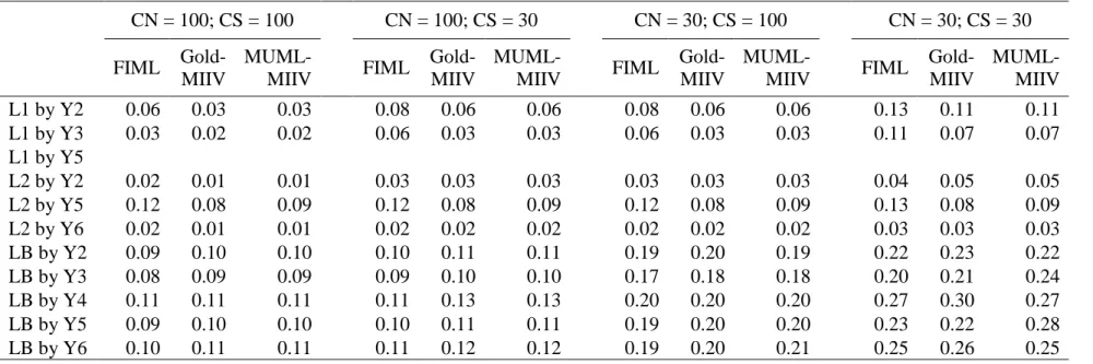
True Model, No Skew/Kurtosis, Balanced Clusters
The first subset of results I examined was the ‘best case’ scenario. Here I compare the
Goldstein-MIIV and MUML-Goldstein-MIIV estimators to FIML in the conditions with no violations of any
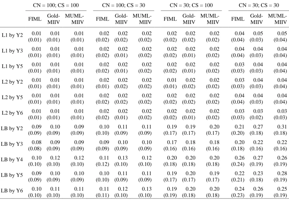
CS for factor loadings. I found evidence that MIIV estimators are performing well across all sample sizes examined. I did not find any mean relative bias across different sample sizes. In general, I note that the spread of relative bias scores increases as sample size decreases, this is normal and to be expected. Additionally, the spread of parameter estimates are slightly larger for MIIV-estimates, as compared to FIML, suggesting a very slight loss of efficiency; this effect is most pronounced at CN=30 and CS=30 and disappears as the cluster size increases. For between level factor loadings I found similar results and less of a difference in terms of efficiency. The difference in variability between within groups factor loadings and between groups factor loadings is also immediately apparent. This is due to the fact that the effective sample size at the between group level is much smaller than at the within level. Across different CN and CS I found negligible mean bias for FIML as well as MIIV estimators. Interestingly, at the smallest sample size in this simulation FIML starts to be positively biased while MIIV estimates have no mean bias.
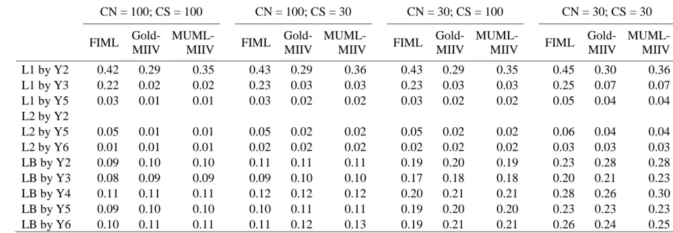
Figure 3 displays relative bias for the variance/covariance parameters. Similar to factor loadings we find these parameters to have no overall mean bias and a similar variability in estimates across estimators. The variance of the between latent factor, ‘LB’, does have a small amount of negative median bias in the CN = 30, CS = 100 condition; despite the median being negatively biased, the mean is still roughly zero. The other general trend we note is that the variability in the between groups latent factor estimates is considerably larger than within, which is due to the smaller effective sample size.
non-existent. This is most pronounced at the smallest N and is least pronounced at the largest N and for between groups factor loadings.
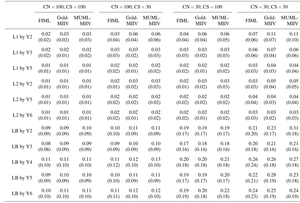
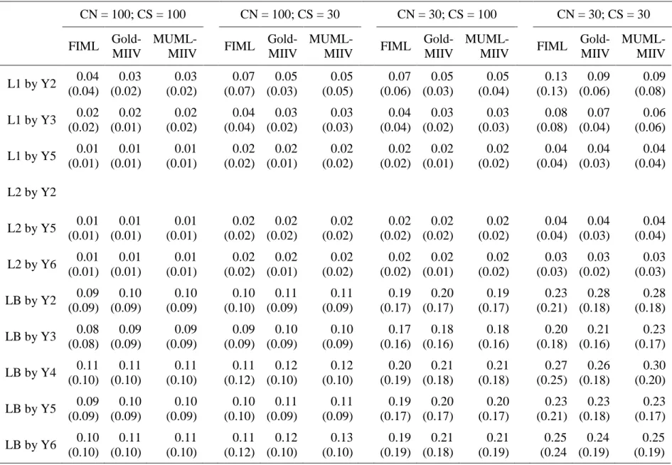
Table 4 reports the empirical standard deviations with the mean standard error reported
from each model. For within factor loadings, FIML and MUML-MIIV standard deviations vs mean standard errors are very close to one another across conditions. This is what I would expect and hope for, because it suggests the reported standard errors reflect the actual variability of estimates. The Goldstein-MIIV estimates had a slight tendency to underreport standard errors for these within factor loadings. In general, Goldstein-MIIV and MUML-MIIV have similar
empirical standard deviations. Goldstein-MIIV then reports a mean standard deviation too small whereas MUML-MIIV reports a mean standard deviation more similar to the actual spread of estimates. At the between level, both MIIV estimators had a tendency to under report standard errors. At the largest sample sizes, this was not much of a problem. However, this became more pronounced as CN/CS decreased and was especially noticeable at CN=30/CS=30. Although, at this sample size even FIML had a tendency to underreport standard errors, but the discrepancy was not as large as it was for MIIV estimators. For the time being it is unclear why this happens. In the future a bootstrap SE or cluster robust SE might do well to help alleviate this disconnect. Performance under structural misspecification
I fit the exact same datasets from above with three different misspecified models, still holding clusters balanced and all data as multivariate normal. This allowed me to assess the effects of model misspecification alone.
relative bias at or greater than 9% for this particular loading. FIML has the most bias, then MUML and then Goldstein. Beyond this single loading directly affected by the misspecification, several other paths have mean bias with FIML; we can see the spread of bias which has been noted as a potential shortcoming of FIML. In contrast to this pattern, for Goldstein-MIIV and MUML-MIIV none of the unaffected paths have mean relative bias. In other words, MIIV’s appear to be more robust to this structural misspecification. Interestingly, the mean percent bias is stable across sample sizes. Finally, FIML had the most mean relative bias at the between level as well (still less than 5%) suggesting a possible cross level contamination of misspecification. MIIV between level loadings are unaffected, suggesting MIIV’s are not as susceptible to such cross level contamination of misspecification.
Table 5 reports the RMSE for this misspecified #1 condition. In addition to being most affected by in terms of mean bias, FIML also has the greatest increase in RMSE—this is mostly true for within factor loadings. Under ideal conditions FIML had general lower RMSE’s;
however with this misspecification, within loadings also have an increase RMSE. Except for the single affect paths for MIIV’s, RMSE stayed almost identical to the true model case. For
between factor loadings, FIML generally still had smaller RMSE, though this difference was still small.
I considered two additional structurally misspecified models. In the second
misspecification I omitted a different factor loading. In the third misspecification I omitted a single correlated error. The findings here reflect much of the same pattern for misspecification #1. For this reason I summarize these misspecified models together and more briefly.
Figure 5 and Figure 6 show relative bias for misspecification #2 and #3 respectively. In misspecification #2 I found a pattern of bias spread similar to misspecification #1 though slightly more severe. The omitted path here occurs with an item that also has a correlated residual, meaning more paths are effect to this omission. As with before we see that bias spreads to more than a single path for FIML but is retained for just a single path with Goldstein-MIIV and MUML-MIIV. Misspecification #3 has the most unique pattern. The two loadings directly affected by the missing correlated residual are biased for all three estimators. Interestingly, the cross loaded path is more biased for MUML-MIIV and Goldstein-MIIV. This was a slightly unexpected result. As with previous models FIML has the most bias for between level factor loadings suggesting a possible cross level spread while this does not happen as much for MIIV estimates.
Taken together these misspecified models generally confirm my hypothesis that MIIV-style estimators would be more robust to structural misspecification. These results are in line with previous simulation studies examining single level SEMs. Additionally, these results suggest that the particular misspecification is an important factor in the performance of all of these estimators. The robustness of the MIIV estimators relies on selecting unaffected
instruments. When the model misspecification affects the instrument selection for many
equations the MIIV estimators are going to be less robust as we saw in misspecification #3. This could perhaps be mitigated by selecting fewer MIIV’s.
Performance under distributional misspecification
For this section the four skew/kurtosis conditions were crossed with CS/CN, holding clusters balanced and only using the true model specification. I ran these conditions with across all sample sizes, however for simplicity tables and figures fix CN=100 and CS=30. Analysis of other cluster sizes revealed that general trends were consistent across cluster size and number of clusters. As a general trend results in this section are similar to pattern seen in the true model condition. Generally bias and RMSE are barely affected, and some of the most pronounced effects can be seen in estimates of variability and uncertainty.
Table 11 reports RMSE for the skew/kurtosis conditions. Here I did not find as much differentiation between the estimators. For a handful of factor loadings I found a slight advantage for FIML (ex., L1 measured by Y2). However for the majority of parameters I found similar RMSE’s across.
Table 12 reports empirical standard deviations and mean standard errors for this condition. Effects of skew and kurtosis were most pronounced for these metrics. In general skew/kurtosis creates more variability in estimates, as expected. However, while there is more variability, mean standard errors do not always reflect this. All three estimators have a tendency to under-report standard errors given these distributional misspecifications. These effects are most pronounced for MIIV estimators and this is especially prominent for the between groups factor loadings given between level skew and kurtosis.
Based on prior research I expected skew of 2 with kurtosis of 8 to have more of an effect than I saw here. Though this result does not confirm the hypothesis, I find it positive to know that all three estimators are generally robust at levels of skew and kurtosis considered high. Often studies of skew and kurtosis in SEM deal more with the effects on global model fit parameters, which I did not examine here (Curran & West, 1996; Ryu, 2011). In single level SEM, Satorra (1990), showed that parameters remained consistent under distributional misspecification (though not structural), and showed that if errors are generated independently from explanatory variables in equation then estimates of precision were also robust. More work could be done to examine more extreme levels of skew and kurtosis.
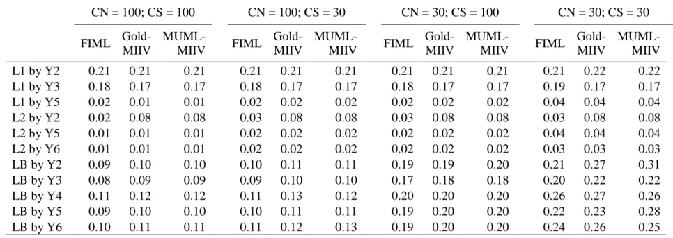
Performance given unbalanced data
unbalance at the levels specified here did not have as much of an effect. I will refer to average cluster size (Avg-CS), implying that the clusters sizes are actually bifurcated around that average. In terms of mean percent relative bias there was no effect for the within groups factor loadings across as Avg-CS and CN. This was expected given that cluster sizes typically have an effect at the between level. At the between level I found low levels of mean relative bias. At the larger sample sizes FIML and MUML-MIIV had slightly more mean relative bias than the Goldstein-MIIV. This trend generalized somewhat to other sample sizes, but was not universal (i.e., for some loadings Goldstein-MIIV had the most mean relative bias). In general I expected Goldstein to be more robust to cluster unbalance, and I found some evidence of this at CN=100, but less evidence at CN=30. I suspect that as CN increases, so does Goldstein’s robustness to cluster unbalance, though future work will have to examine this more closely.
Table 13 contains the RMSE’s for unbalanced cells. I continued to find the general trend that FIML has lower RMSE’s at the within level, although in most cases this difference was
slight. Between level factor loadings had almost no differentiation between RMSE at the highest Avg-CS/CN; at Avg-CS=30 and CN=30 I found the opposite effect that Goldstein and MUML generally have smaller RMSE.
under-report standard errors. This trend is actually most pronounced for FIML which has the largest empirical standard deviation of between groups factor loading estimates.
Examining Sargan’s test performance
Sargan’s test for misspecification is a major advantage of using MIIV estimation. While
FIML offers global fit statistics, if researchers have over-identified equations with MIIV’s then they have the ability to test for local misspecification one equation at a time. Given that MIIV estimation has never been done for multilevel CFA. I wanted to examine the performance of the test with these estimation procedures. Obviously, Sargan’s test was not developed with the
procedure of decomposing data into within groups and between groups covariance matrices. That is, I was unsure if the proposed estimators would meet the usual assumptions of Sargan’s test and
still provide a useful tool in this context. To examine the functioning of Sargan’s test I summarize the percent rejection rates for each indicator across various conditions.
factor loadings, MUML-MIIV alpha rates stay consistently around 0.05 across all sample sizes, and the Goldstein-MIIV alpha rates remain elevated. The failure of the Goldstein MIIV Sargan’s test is a bit perplexing given the relative success of the MUML-MIIV. This is likely related to the smaller reported standard errors—correcting the standard errors in the Goldstein procedure will likely help alleviate the shortcomings of Sargan’s here. This problem persists throughout the rest of the comparisons.
The true advantages of using Sargan’s test are more apparent in Figure 10, Figure 11 and
Figure 12, which illustrate alpha levels across the various misspecifications. The general trends found in the true model specification remain, however for each of the misspecification Sargan’s test flags one or more paths as misspecified. In misspecification #1, both Goldstein-MIIV and MUML-MIIV flag the L2 measured by Y5 path 100% of the time. Recall that the misspecified path in this model is the cross loading L1 measured by Y5. Looking back at Figure 2, the mean relative bias plot for misspecification #1, we see that L2 measured by Y5 is the only path which is biased for MIIV estimators. This pattern is the similar across misspecification #2 and #3. Sargan’s test flags paths which also happen to be the most biased paths in the model.
Finally, Figure 13 and Figure 14 display the performance of Sargan’s test given
skew/kurtosis and cluster unbalance respectively. Skew and kurtosis raises the rejection rates for the level of factor loadings with skew/kurtosis. As with Goldstein, this may be related to
Chapter 3: Conclusions
Full information maximum likelihood has become the de facto estimation routine for multilevel CFA, and this is not without reason. We know that given the correct model and no excessive multivariate kurtosis, FIML will be asymptotically efficient and asymptotically unbiased. FIML handles missing data effortlessly. FIML can incorporate random slopes and more than two levels. FIML is flexible and in many circumstances it makes perfect sense that it is used widely. However, I have tried to make the argument that despite its usefulness and flexibility it also makes strong assumptions. Without meeting these assumptions, researchers have no guarantee about the asymptotic efficiency and asymptotic unbiasedness of FIML
estimates. Therefore, in circumstances when it is possible to use limited information estimators it may make sense to do so.
Limited information estimators have been shown to be excellent estimators often requiring fewer and less rigid assumptions (Bollen 1996a). In this paper I developed and evaluated two such estimators: The Goldstein-Model Implied Instrumental Variable Estimator and the MUML-Model Implied Instrumental Variable estimator. Following analytic
developments of the MIIV estimator for single level SEM’s, I developed two novel procedures for using MIIV’s to estimate multilevel CFA models. Finally, I evaluated both new estimators in
MIIV approaches as implemented here cannot. FIML can incorporate more than two levels and MIIV approaches here cannot. FIML can easily handle missing data while MUML-MIIV would need multiple imputation. This is to say that MUML-MIIV and Goldstein-MIIV may be useful for many multilevel CFA models but cannot compete with the general flexibility of FIML and thus FIML is certainly still necessary in many multilevel CFA models, particularly more complex models.
That said, our results suggest that both MIIV estimators performed well in the conditions I considered, with the MUML-MIIV being a clear favorite between the two. Starting with the best case scenario (i.e., True model, no distributional misspecification, and balanced clusters), Goldstein-MIIV and MUML-MIIV performed comparably to FIML. This best-case scenario is unlikely to resemble modeling in practice as it is highly unlikely we ever have the true model. However, this was an opportunity to compare ideal properties. The MIIV estimators had a slight loss in efficiency as compared with FIML, however the difference was minute, found mostly in this true model condition. The real advantages of using the MUML-MIIV or Goldstein-MIIV estimators was apparent in the misspecified model conditions. In these cases, which are arguably much more likely to resemble CFA with real data, I found that MIIV estimators were much more robust to bias due to misspecification. When we do not know the ‘True’ model, it is all but guaranteed that our models will include some misspecification. These types of scenarios are the norm, and they happen to be when the MIIV estimators outperformed FIML.
My results were largely focused on factor loadings as the primary outcome, although I also considered variance covariance parameters in the True Model condition. These results indicated that we could also estimate variance covariance parameters with MIIV’s similarly to
with MIIV procedure requires an additional stage in the estimation process, where factor loadings are treated as fixed and covariance parameters are estimate. This is an additional stage in an estimation routine that already has 3 stages. Though our results suggest variance covariance parameters were estimated with no mean bias and similar efficiency to FIML, in some cases the multi-stage process might cause more issue. Additionally, standard errors are not as easy to obtain on variance components with MIIVs. We did not compute them here, though it is possible to estimate them with bootstrapping. FIML, on the other hand, provides these for free.
Despite the positive performance of both MIIV estimators in terms of mean relative bias and RMSE, they did have a problematic tendency to underestimate standard errors. For MUML-MIIV this tendency was most noticeable at small sample sizes for between groups factor
loadings and given non-normality and cluster unbalance. In addition to those circumstances, Goldstein-MIIV had a slight tendency to underestimate standard errors for within loadings even at large sample sizes. It should be noted that even FIML had a tendency to underestimate standard errors for between groups factor loadings at CS=30, albeit the discrepancy was less. Though corrections are likely possible for the MIIV estimators, it is also possible that thirty clusters is an inadvisably low number of clusters for fitting complex multilevel factor models. Obviously, underestimating standard errors is problematic and something which needs to be considered heavily. Future studies will need to investigate this further and perhaps consider corrections such as bootstrapping which has its own complications with multilevel data (van der Leeden, Meijer, & Busing, 2008).
with an indicator with a cross loading created more bias for FIML and more bias for MIIVs (though still less than FIML). Finally, an omitted correlated residual created the most mean bias for all three estimators, and in one particular path MIIV’s had more mean bias than FIML. While MIIV’s in general had less mean bias due to misspecification, MIIVs did not always have the
least mean bias, and it may vary model to model.
Additionally, there are a variety of types of misspecification and no study is able to simulate all the possible discrepancies models and reality. This study and many MIIV-2SLS studies have been more focused on model misspecification as it arises from omitting true relationships and included null relationships. It might be that this is the type of misspecification MIIV-2SLS is most robust to. However, discrepancies between models and reality can come in many forms (Cudeck & Henly, 1991; Linhart & Zucchini, 1986; MacCallum, 2003; MacCallum & Tucker, 1991; Meehl, 1990). MacCallum (2001) discussed the importance of considering model imperfection and offers an excellent overview of many others who have considered this. Macallum and Tucker (1991) call the lack of correspondence between reality and our simplified models model error. Cudeck and Henly (1991) call the same phenomena approximation
discrepancy. MacCullum and Tucker (1991) discussed five sources of model error concluding
misspecifications and model errors to more fully understand how MIIV-2SLS performs given a variety of model errors.
There may be more ways to control the spread of bias with MIIV’s that were not employed in this particular study. Bias with MIIV’s is a direct result of the instruments used in each equation. When bad instruments are used, this creates bias for MIIVs. In this study, to estimate each within equation, I used all possible MIIVs. This increases the chance of using a bad instrument, and increasing the chance that bias may spread. One possible option would be to limit the subset of MIIVs to be a smaller subset, decreasing the chances that bias spreads (though not a guaranteed result). Although, this has the negative consequence that Sargan’s test is less useful in identifying model misspecification. Future research should examine particular strategies for deciding how many MIIVs to include.
Given model misspecification, I cannot overlook the importance of Sargan’s test as a
useful tool when using MIIV estimation. In the single level case, Sargan’s Test has been shown to offer a more specific strategy for testing model fit as opposed to typical global fit statistics. At the outset, I was not sure if the conditions of splitting covariance matrices at two levels, would meet the typical assumptions of Sargan’s test. In this simulation I showed that there was a direct
correspondence to Sargan’s test flagging misspecification and biased paths. Sargan’s test with MUML-MIIV also had roughly appropriate alpha levels, while the Sargan’s with Goldstein-MIIV had elevated alpha levels. In general, Sargan’s offers researchers an excellent way to test