K. Joost Batenburg1,2, Leon Helwerda3, Walter A. Kosters3 ( ), and Tim van der Meij3
1
Mathematical Institute, Leiden, the Netherlands
2
CWI, Amsterdam, the Netherlands
3
Leiden Institute of Advanced Computer Science (LIACS), Leiden, the Netherlands [email protected]
Abstract. Mobile radio tomography applies moving agents that perform wireless signal strength measurements in order to reconstruct an image of objects inside an area of interest. We propose a toolchain to facilitate automated agent planning, data collection, and dynamic tomographic reconstruction. Preliminary experiments show that the approach is feasible and results in smooth images that clearly depict objects at the expected locations when using missions that sufficiently cover the area of interest.
Keywords: radio tomography, intelligent agents, wireless signal strength measurements, image reconstruction, localization and mapping
1
Introduction
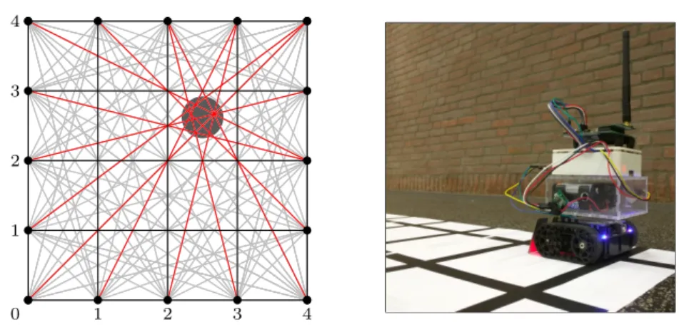
Radio tomographyis a technique for measuring the signal strength of low-frequency radio waves exchanged between sensors around an area, and reconstructing information about objects in that area. We send a signal between a source and target sensor of a bidirectional link. The signal passes through objects that attenuate it, resulting in a detectably weaker signal at the receiving end. This phenomenon makes it possible to determine where objects are located. The typical setup for radio tomography is illustrated in Fig. 1 (left), in which the sensors are situated on the boundaries in an evenly distributed manner. Gray lines represent unobstructed links and red lines indicate links attenuated by the object.
Radio tomography has several benefits over other detection techniques. We can see through walls, smoke or other obstacles. The technique does not require objects to carry sensor devices. The radio waves are non-intrusive, with no permanent effects on people. The technique is less privacy-invasive than optical cameras as the possible level of detail is inherently limited due to the nature of the radio waves. It is not possible to accurately identify a person, but we do aim for reconstructed objects that we recognize as such.
0 1 2 3 4
1 2 3 4
Fig. 1: The sensor network and the physical realization of a vehicle.
One way to resolve these issues is to move the sensors around using agents, which are realized as autonomous vehicles as pictured in Fig. 1 (right). We position them along a grid which defines discrete and precise sensor positions. These positions produce a matrix of coordinate-basedpixels in the reconstructed image. In comparison to the static setup, we require fewer sensors and less prior knowledge about the area. We may adapt the coverage dynamically, for example by zooming in on a part of the area. We name this conceptmobile radio tomography, which includes both the agent-based measurement collection and the dynamic reconstruction approach.
In this paper, we present our toolchain for mobile radio tomography using intelligent agents, as an engineering effort that builds upon and combines several techniques. In Sect. 2 we describe the key challenges for mobile radio tomography and the components in our toolchain that address them. We then cover two such challenges in greater detail: (i) planning the paths of the agents in Sect. 3, and (ii) reconstructing an image from the measurements in Sect. 4. Results for real-world experiments are presented in Sect. 5, followed by conclusions and further research in Sect. 6. This paper is based on two master’s theses on the subject of mobile radio tomography [10,14].
2
Toolchain
and certainly noisy. Synchronization between the agents must be interleaved with data acquisition using a robust communication protocol.
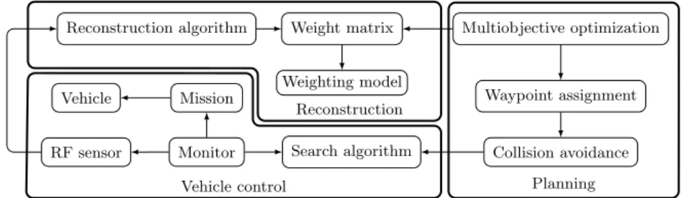
To deal with these challenges, we developed an open-source, component-based toolchain. The toolchain is mainly written in Python, with low-level hardware components written in C. The diagram in Fig. 2 shows the toolchain’s components.
Vehicle
RF sensor
Mission
Monitor Search algorithm Reconstruction
Vehicle control
Collision avoidance Waypoint assignment Multiobjective optimization
Planning Weight matrix
Weighting model Reconstruction algorithm
Fig. 2: Diagram of components in the toolchain.
The planning components generate missions for signal strength measurements, as discussed in Sect. 3. The problem of devising a set of link positions to measure is solved by an evolutionary multiobjective algorithm that simulates reconstruction models to ensure that the links cover the entire network. Next, a waypoint assignment algorithm distributes the sensor positions for each link over the vehicles. A path graph search algorithm prevents the vehicles from clashing.
Execution of the mission is taken care of by the vehicle control components. The monitor oversees the process and tracks auxiliary sensors on the vehicles, such as distance sensors for obstacle detection. It makes the RF (radio frequency) sensor perform the signal strength measurements and it may use the search algorithm for collision avoidance during a mission. The mission consists of the waypoints for the vehicle and provides instructions to the vehicle controller. During a mission, this causes the vehicle to move toward the next waypoint.
The reconstruction component converts the signal strength measurements to a two-dimensional visualization of the area of interest. We describe this process in detail in Sect. 4. The weight matrix determines which pixels are intersected by a link, and a weighting model describes how the contents of pixels contribute to a measured signal strength.
3
Missions
perform measurements together while traversing short and safe paths that do not conflict with concurrent routes. This problem is related to various multi-agent vehicle routing problems with synchronization constraints [6,9,13]. We propose a two-stage algorithm, and describe both parts in text as well as pseudocode.
We assume that we know which links we measure for collecting tomographic data; later on we generate these links using an evolutionary algorithm. To measure a link, sensors must be placed at two positions at the same time. We distribute these tasks over the vehicles. Our assignment algorithm is given as input a set
P ={(p1,1, p1,2),(p2,1, p2,2), . . . ,(pω,1, pω,2)} (1)
withω location pairs ofcoordinate tuples (two-dimensional vectors), and a set
V = {v1, v2, . . . , vη} of η ≥ 2 vehicles, initially located at coordinate tuples
S1, S2, . . . , Sη. Now defineU ={(u, v)|u∈V, v∈V, u6=v}, the pairwise unique permutations of the vehicles, e.g., with two vehicles, this isU ={(v1, v2),(v2, v1)}.
Our greedy assignment in Algorithm 1 then works as follows: for each vehicle pair ϑ= (va, vb)∈U and each sensor pairρ= (pc,1, pc,2) ∈P, determine the distances d1(ϑ, ρ) = kSa−pc,1k1 and d2(ϑ, ρ) = kSb−pc,2k1. We use the L
1
normk·k1 to only move in cardinal directions on a grid; in other applications we may use theL2normk·k
2. Next, take the maximal distance (since one agent must wait for the other to perform a measurement), and finally select the overall minimal pair combination, i.e., solve the following optimization problem:
arg min (ϑ,ρ)∈U×P
max(d1(ϑ, ρ), d2(ϑ, ρ))
(2)
Algorithm 1 Greedy waypoint assignment
1: procedureAssign(S1, S2, . . . , Sη, P, V)
2: letAibe a sequence of waypoints for each vehiclevi, withi= 1,2, . . . , η 3: U ← {(u, v)|u∈V, v∈V, u6=v}
4: whileP 6=∅do
5: δm← ∞
6: for all(ϑ, ρ)∈U×P do . ϑ= (va, vb) andρ= (pc,1, pc,2)
7: d←max(kSa−pc,1k1,kSb−pc,2k1)
8: if d < δmthen
9: δm←d,ϑm←ϑandρm←ρ
10: end if
11: end for . ϑm= (va, vb) andρm= (pc,1, pc,2)
12: appendpc,1 to the assignmentAa for vehicleva 13: appendpc,2 to the assignmentAb for vehiclevb 14: Sa←pc,1 andSb←pc,2
15: removeρmfrom the setP
16: end while
The selected positions are then assigned to the chosen vehicle pair, and removed from P. Additionally,Sa becomes the first position andSb becomes the second sensor position. The greedy algorithm then continues with the next step, untilP
is empty, thus providing a complete assignment for each vehicle.
Secondly, we design a straightforward collision avoidance algorithm that searches for routes between waypoints that do notconflict with any concurrent route of another vehicle; see Algorithm 2. The algorithm is kept simple in order to incorporate it into an evolutionary algorithm (see [7,12] for more intricate methods which result in optimized routes). We use a path graph search algorithm to find a safe route that crosses no other routes. Once a vehicle performs a measurement involving another vehicle, their prior routes no longer conflict.
Algorithm 2 Collision avoidance
1: procedureAvoid(V, S1, S2, . . . , Sη, vp, vq, Np)
2: letW1, W2, . . . , Wηbe sets, withWi={vi}fori= 1,2, . . . , η
3: letGbe a graph of discrete positions and connections in the area 4: remove incoming edges of nodes inGthat enter forbidden areas 5: remove incoming edges ofS1, S2, . . . , Sη fromG
6: letR1, . . . , Rη be empty sequences of routes
7: for allvi∈V \Wpdo
8: remove the edges for nodes inRifromG
9: end for
10: R∗←Search(G, Sp, Np) .find a safe pathR∗inGfromSptoNp 11: appendR∗toRp
12: reinsert the edges forSpinto the graphG 13: remove incoming edges for the nodeNp 14: Sp←NpandWp←Wp∪ {vq} 15: for allvi∈V do
16: if vi∈/Wpthen
17: reinsert the edges for nodes traversed by the pathRi intoG
18: end if
19: if vi6=vpandWi=V then 20: clear the sequenceRi
21: Wi← {vi}
22: end if
23: end for
24: returnRp
25: end procedure
We use the collision avoidance algorithm every time the waypoint assignment algorithm assigns a position to a vehicle, so twice per step. Thus, we detect problematic situations as they occur, which are either solved via detours (although the vehicle might also search for a faster safe path while the mission takes place), or by rejecting the entire assignment. The resulting assignments should be collision-free, assuming that all vehicles follow their assigned route and wait for each other at synchronization points, where they also perform their signal strength measurements.
In order to supply the waypoint assignment algorithms with a non-static set of sensor positions P (see (1)), we utilize an evolutionary multiobjective algorithm [8]. The iterative algorithm generates a set of positions and alters it in such a way that it theoretically converges toward an optimal assignment. We keep a population (X1, X2, . . . , Xµ) of multiple individuals, each of which contains variables that encode the positions in an adequate form. After a random initialization, the algorithm performs iterations in which it selects a random individualXi and slightly mutates it to form a new individual [2].
In our situation, the variables of an individual encode coordinates for positions around the area of interest, and possibly inside of it as well. Definem(i)as the number of pairs of positions that are correctly placed, such that the link between the positions intersects the network. Using these positions, we can deduce other information, such as a weight matrixA(i)(containing link influence on pixels; see Sect. 4), for each individualXi. The algorithm then removes an individual that is infeasible according to the domain of the variable or due to the constraints
in (3) and (4), such as a minimum number of valid linksζ. The constraints are wrapped into a combined feasibility value in (5):
Q(i)1 :∃j:∀k:Aj,k(i) 6= 0 (3) Q(i)2 :m(i)≥ζ (4)
fi=
(
0 if¬Q(i)1 ∨ ¬Q(i)2
1 ifQ(i)1 ∧Q(i)2 (5)
In the case that all constraints and domain restrictions are met by each individual, the multiobjective algorithm uses a different selection procedure based on the
objective functions. We remove an individual if its objective values are strictly higher than those of one dominating individual in the population. If none of the individuals are dominated, we remove the one with the minimum crowding distance [5]. The crowding distance is defined as the area around the individual within the objective space. We can place the objective values in this space as a plotted function, which is known as thePareto front.
g1(Xi) =− m(i) X
j=1 n
X
k=1
A(i)j,k (6)
g2(Xi) =δ·
m(i) X
j=1
p
(i) j,1−p
(i) j,2
2
+ (1−δ)·T(i) (7)
In the entire selection step of the evolutionary algorithm, we use the reconstruction, waypoint assignment and collision avoidance algorithms to check that a new individual adheres to the constraints and to calculate the objective values. Aside from the link weight matrixA(i)for one individualXi, we calculate the pairwiseL2norms between sensor positions, andT(i), the sum of minimized route distances (2), weighted by a factor δ. These algorithms generate missions that provide sufficient network coverage. When we stop the evolutionary multiobjective algorithm, we can manually select one of the individuals and use the mission it generates, using the Pareto front as a reference for balanced objective values [5].
4
Reconstruction
The reconstruction phase takes care of converting a sequence of signal strength measurements to a two-dimensional image of size m×n pixels that may be visualized. LetM ={(s1, t1, r1), . . . ,(sk, tk, rk)}be the input, in whichsi andti are pairs of integers indicating thexandycoordinates on the grid for the source and target sensori, respectively,riis thereceived signal strength indicator(RSSI) andkis the total number of measurements. We express the conversion problem algebraically asAx=b. Here,bis a column vector of RSSI values (r1, r2, . . . , rk)T,
xis a column vector ofm·npixel values (in row-major order) andAis a weight matrix that describes how the RSSI values are to be distributed over the pixels that are intersected by the link, according to a weighting model.
In general, signal strength measurements contain a large amount of noise due to
multipath interference. The wireless sensors send signals in all directions, and thus more signals than those traveling in the line-of-sight path may reach the target sensor, causing interference. This phenomenon is especially problematic in indoor environments due to reflection of signals. Although techniques exist to include an estimate of the contribution of noise inside the model [15], we suppress noise outside the model using calibration measurements and regularization algorithms. The difficulty lies in the fact that the reconstruction problem is an ill-posed inverse problem, which we have to solve for highly noisy and unstable measurements.
Theweight matrix Adefines the mapping between the inputband the output
x. If and only if the contents of a pixel with indexiattenuate a link with index`, then the weightw`,iin row`and columniis nonzero. Given a link`, aweighting
shorter links [16]. The variable d`,i is the sum of distances from the center of pixelito the two endpoints of link`.
The line model in (8) assumes that the signal strength is determined by objects on the line-of-sight path, as shown in Fig. 3a; theellipse model in (9) is based on the definition of Fresnel zones:
w`,i=
(
1 if link`intersects pixel i
0 otherwise (8)
w`,i=
(
1/√d` ifd`,i< d`+λ
0 otherwise (9) w`,i=e
−(d`,i−d`)2/2σ2 (10)
Fresnel zones, used to describe path loss in communication theory, are ellipsoidal regions with focal points at the endpoints of the link and a minor axis diameter
λ. Only pixels inside this region are assigned a nonzero weight, as seen in Fig. 3b.
0 1 2 3 4 5 6 7 8 9 10 11 12 13 14 15 16 0 1 2 3 4 5 6 7 8 9 10 11 12 13 14 15 16
(a) Line model
0 1 2 3 4 5 6 7 8 9 10 11 12 13 14 15 16 0 1 2 3 4 5 6 7 8 9 10 11 12 13 14 15 16 0 0.1 0.2 0.3
0.4 0.5 0.6 0.7 0.8 0.9 1 Weight
(b) Ellipse model
0 1 2 3 4 5 6 7 8 9 10 11 12 13 14 15 16 0 1 2 3 4 5 6 7 8 9 10 11 12 13 14 15 16 0 0.1 0.2 0.3
0.4 0.5 0.6 0.7 0.8 0.9 1 Weight
(c) Gaussian model
Fig. 3: Illustration of weight assignment for a link from (0, 0) to (16, 16) by the weighting models.
Moreover, we introduce a newGaussian model in (10). This model is based on the assumption that the distribution of noise conforms to a Gaussian distribution. The log-distance path loss model is a signal propagation model that describes this assumption as well [1].
Due to the ill-posed nature of the problem, in general there exists no exact solution forAx=bbecauseA is not invertible. Instead, we attempt to find a solutionxmin that minimizes the error usingleast squares approximation [3] as defined in (11), whereR(x) is a regularization term:
xmin= arg min
x
kAx−bk22+R(x) (11)
Thesingular value decomposition (SVD) ofAmay be used to solve this and is defined as A=U ΣVT, in whichU andV are orthogonal matrices andΣ is a diagonal matrix with singular values [16]. If we use the exact variant of singular value decomposition which does not apply any regularization, then we have the regularization termR(x) = 0.Truncated singular value decomposition (TSVD) is a regularization method that only keeps theτ largest singular values in the SVD and is defined asA=UτΣτVτT [16]. Small singular values have low significance for the solution and become erratic when taking the reciprocals forΣ. Moreover, the truncated singular value decomposition is faster to compute, which is an important property for reconstructing images in real time.
While the dimensionality reduction from TSVD does stabilize the solution, the resulting images may still contain unstable spots. Iterative regularization methods incorporate desired characteristics of the reconstructed images.Total variation minimization (TV, see [16]) enforces that the reconstructed images are smooth, i.e., that the differences between neighboring pixels are as small as possible, by favoring solutions that minimize variability in the resulting image. The gradient ∇xofxis a measure of the variability of the solution. The regularization term
in (11) is set to R(x) = αPξ−1
i=0
q
(∇x)i2+β, in which ξ is the number of elements in∇x. The parameterαindicates the importance of a smooth solution and leads to a trade-off as a high value indicates more noise suppression, but less correspondence to the actual measurements. The term is not squared, so we need an optimization algorithm for the minimization. The parameterβ is a small value that prevents discontinuity in the derivative whenx= 0, as that generally needs to be supplied to optimization algorithms.
Finally, let us consider another measure of variability. Maximum entropy minimization (ME) smoothens the solution by minimizing its entropy. Entropy is a concept in thermodynamics that provides a measure of the amount of disorder in a structure. The Shannon entropy is defined as H = −Pγ−1
5
Experiments
To study the effectiveness of our approach, we perform a series of experiments. Two vehicles drive around on the boundaries of a 20×20 grid in an otherwise empty experiment room. We use hand-made missions that apply common patterns used in tomography, such as fan beams. With this setup we create a dataset with two persons standing in the middle of the left side and in the bottom right corner of the network, and a dataset with one person standing in the top right corner of the network. A separate dataset is used for calibration.
The first experiment compares all combinations of regularization methods and weighting models to determine which pair yields the most accurate reconstructions. We use the dataset with the two persons, so both must be clearly visible. The outcomes of this experiment are presented in Fig. 4, in which darker pixels indicate low attenuation and brighter pixels indicate high attenuation.
(a) SVD, line (b) TSVD, line (c) TV, line (d) ME, line
(e) SVD, ellipse (f) TSVD, ellipse (g) TV, ellipse (h) ME, ellipse
(i) SVD, Gaussian (j) TSVD, Gaussian (k) TV, Gaussian (l) ME, Gaussian
The first observation is that SVD indeed leads to major instabilities because of the lack of regularization. Noise is amplified to an extent that the images do not provide any information about the positions of the persons. TSVD, while being a relatively simple regularization method, provides more stable resulting images that clearly show the positions of the two persons. The ellipse model and the new Gaussian model yield similar clear results, whereas using the line model leads to slightly more noise compared to the former two. Even though TV and ME use different variation measures, the reconstructions are visually the same and equally clear.
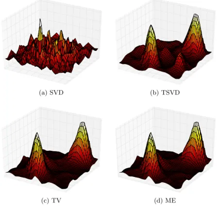
Besides providing a clear indication of where the persons are located inside the network, it is important that the reconstructed images are smooth. The second experiment studies the smoothening effects of the regularization methods using 3D surface plots of the raw grayscale images, i.e., without any additional coloring steps applied. The only difference between the experiment runs are the regularization method, so any other parameters remain the same, such as the Gaussian weighting model and the precollected dataset with the two persons that we use as input. The results for this experiment are shown in Fig. 5.
(a) SVD (b) TSVD
(c) TV (d) ME
The ideal surface plot consists of a flat surface with two spikes exactly at the positions of the persons. The surface plot for SVD is highly irregular, which leads to noticeable noise in the image due to a high variance in pixel values. In contrast, the surface plot for TSVD is smooth and the two spikes are clearly distinguishable. However, there are still some small unstable spots. The surface plots for TV and ME are, again, practically the same and have even fewer instabilities.
With regard to the algorithmically generated missions discussed in Sect. 3, we perform a parameter optimization by comparing the average objective values of the resulting individuals in multiple runs of the evolutionary algorithm. The twelve parameters influence the sensitivity and scale of the optimization algorithm, as well as the waypoint assignment and collision avoidance algorithms. Certain features, such as a mutation operator specially designed to optimize link positions, can be enabled and disabled this way as well. We provide 350 unique combinations of values to these parameters, and repeat each experiment five times.
We find that some of these variables influence the performance in terms of stability, convergence speed and finding optimized positions. For example, the specialized mutation operator finds individuals that have better objective values, but result in chaotic populations over time. The population size hardly affects the algorithm’s effectiveness nor speed. Other parameters produce missions which are applicable only if we change the dimensions of the area of interest.
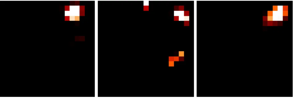
For the final experiment, we generate a mission for a 20×20 grid using the evolutionary multiobjective algorithm, and compare it to a hand-made mission used previously. The algorithm is tuned to place sensors for at least 320 and up to 400 valid links to be measured during the mission. The results of the parameter optimization are applied as well. At 7000 iterations, we end the generation run and pick aknee point solution that optimizes both objectives in the resulting Pareto front. A manual check using the collision avoidance algorithm determines that this assignment is safe. In Fig. 6, we show the images resulting from the tomographic reconstruction of the dataset with one person.
(a) Algorithmically planned mission, halfway result
(b) Hand-made mission, halfway result
(c) Hand-made mission, final result
The reconstruction, which is run in real time during the collection of signal strength measurements, uses TV and the Gaussian model. We can track the time it takes before a mission provides a smooth and correct result, in terms of quality and realism. In Fig. 6a, we are around halfway through the planned mission, with 204 out of 382 measurements collected. The reconstructed image clearly shows the person standing in the top right corner. Fig. 6b shows the reconstructed image provided by the hand-made mission after 413 out of 800 measurements. Although this mission’s movements are less erratic (and more measurements per time unit are made), it is not stable enough to clearly show one person while it develops. Fig. 6c shows the end result, where the hand-made mission does provide an acceptable reconstructed image. The planned mission does not diverge from its initial smooth image and we can stop the mission early.
6
Conclusions and Further Research
We propose a mobile radio tomography toolchain that collects wireless signal strength measurements using dynamic agents, which are autonomous vehicles that move around with sensors. We plan missions, which describe the locations that the agents must visit and in what order. Novel algorithms provide us with generated missions, guaranteeing that two sensors are at the right locations to perform a measurement. The algorithms avoid conflicts between the routes and provide an optimized coverage of the network.
The measurements are passed to the reconstruction algorithms to create a visualization of the area of interest that corresponds to the patterns in the data as best as possible. Regularization methods suppress noise in the measurements and increase the smoothness of the resulting image. We introduce a new Gaussian weighting model and apply maximum entropy minimization to the problem of radio tomographic imaging. Preliminary experiments show that the mobile radio tomography approach is effective, i.e., it is able to provide smooth reconstructed images in a relatively short time frame using algorithmically planned missions.
There is much potential for further research. One interesting topic is to replace the agents, that currently operate on the ground using small-scale robotic rover cars, with drones that fly at different altitudes. This leads to 3D reconstruction, e.g., by performing a reconstruction at different altitudes and combining the images, which are slices of the 3D model. The reconstruction algorithms could be modified to allow performing measurements anywhere in the 3D space, although this makes the problem more difficult to solve in real time.
References
1. Andersen, J.B., Rappaport, T.S., Yoshida, S.: Propagation measurements and models for wireless communications channels. IEEE Communications Magazine 33, 42–49 (1995)
2. B¨ack, T.: Evolutionary algorithms in theory and practice: Evolution strategies, evolutionary programming, genetic algorithms. Oxford University Press (1996) 3. Bj¨orck, A.: Numerical methods for least squares problems. SIAM (1996) 4. Bovik, A.C.: Handbook of image and video processing. Academic Press (2005) 5. Branke, J., Deb, K., Dierolf, H., Osswald, M.: Finding knees in multi-objective
optimization. In: Proceedings of the International Conference on Parallel Problem Solving from Nature. LNCS, vol. 3242, pp. 722–731. Springer (2004)
6. Bredstr¨om, D., R¨onnqvist, M.: Combined vehicle routing and scheduling with temporal precedence and synchronization constraints. European Journal of Operational Research 191, 19–31 (2008)
7. De Wilde, B., ter Mors, A.W., Witteveen, C.: Push and rotate: Cooperative multi-agent path planning. In: Proceedings of the 2013 International Conference on Autonomous Agents and Multi-agent Systems, pp. 87–94. International Foundation for Autonomous Agents and Multiagent Systems (2013)
8. Emmerich, M., Beume, N., Naujoks, B.: An EMO algorithm using the hypervolume measure as selection criterion. In: Proceedings of the Third International Conference on Evolutionary Multi-Criterion Optimization. LNCS, vol. 3410, pp. 62–76. Springer (2005)
9. Golden, B.L., Raghavan, S., Wasil, E.A.: The vehicle routing problem: Latest advances and new challenges. Springer (2008)
10. Helwerda, L.: Mobile radio tomography: Autonomous vehicle planning for dynamic sensor positions. Master’s thesis, LIACS, Universiteit Leiden (2016)
11. Menegatti, E., Zanella, A., Zilli, S., Zorzi, F., Pagello, E.: Range-only SLAM with a mobile robot and a wireless sensor networks. In: Proceedings of the 2009 IEEE International Conference on Robotics and Automation, pp. 8–14 (2009)
12. Sharon, G., Stern, R., Felner, A., Sturtevant, N.R.: Conflict-based search for optimal multi-agent pathfinding. Artificial Intelligence 219, 40–66 (2015)
13. Standley, T.S.: Finding optimal solutions to cooperative pathfinding problems. In: Proceedings of the Twenty-Fourth AAAI Conference on Artificial Intelligence, pp. 173–178 (2010)
14. Van der Meij, T.: Mobile radio tomography: Reconstructing and visualizing objects in wireless networks with dynamically positioned sensors. Master’s thesis, LIACS, Universiteit Leiden (2016)
15. Wilson, J., Patwari, N.: Radio tomographic imaging with wireless networks. IEEE Transactions on Mobile Computing 9, 621–632 (2010)