CHOOSING A CONTRACEPTIVE PROVIDER:
ACCESS, AWARENESS AND FERTILITY DECISIONS IN URBAN SENEGAL
Rayan Joneydi
A dissertation submitted to the faculty of the University of North Carolina at Chapel Hill in par-tial fulfillment of the requirements for the degree of Doctor of Philosophy in the Department of Economics.
Chapel Hill 2018
Approved by: David K. Guilkey Clement J. E. Joubert Luca Flabbi
ABSTRACT
Rayan Joneydi: Choosing a Contraceptive Provider: Access, Awareness and Fertility Decisions in Urban Senegal (Under the direction of David K. Guilkey and Clement J. E. Joubert)
ACKNOWLEDGEMENTS
TABLE OF CONTENTS
LIST OF TABLES . . . viii
LIST OF FIGURES . . . x
1 INTRODUCTION . . . 1
2 RELATED LITERATURE . . . 5
2.1 Access to Quality and Contraceptive Use . . . 5
2.2 Quality of Care Framework . . . 7
3 MODEL . . . 9
3.1 Environment and Choice Set . . . 9
3.2 State Variables . . . 10
3.3 Preferences . . . 11
3.4 Program Exposure . . . 12
3.5 Pregnancies . . . 13
3.6 Initial Conditions and Types . . . 13
3.7 The Optimization Problem . . . 14
4 DATA . . . 17
4.1 Country Overview . . . 17
4.2 The MLE Project . . . 17
4.3 Sample Selection . . . 19
4.4 Model Variables . . . 22
4.5 Provider Choice . . . 25
5 REDUCED-FORM ANALYSIS . . . 31
6 STRUCTURAL ESTIMATION . . . 35
6.1 Likelihood Function . . . 35
6.2 Identification . . . 35
7 RESULTS . . . 37
7.1 Parameter Estimates . . . 37
7.2 Model Fit . . . 39
8 POLICY EXPERIMENTS . . . 44
9 CONCLUSION . . . 48
APPENDIX . . . 50
LIST OF TABLES
4.1 Sample Selection Process . . . 20
4.2 Person-Year Observations . . . 21
4.3 Provider Sample . . . 21
4.4 Provider Choice Set . . . 22
4.5 Permanent Demographic Characteristics . . . 23
4.6 Time-Varying Demographic Characteristics . . . 24
4.7 Provider Variables . . . 25
4.8 Provider Types (%) . . . 26
4.9 Provider Choice by Wealth Status . . . 27
4.10 Nearest vs. Chosen Provider in 2015 (Among Users Who Bypass) . . . 27
4.11 Communication With Husband and Agency Over Reproductive Decisions at Base-line (%) . . . 30
5.1 Impact of Different Family Planning Programs . . . 33
5.2 Impact Mechanisms . . . 34
7.1 Permanent Characteristics by Simulated Type . . . 38
7.2 Choices, Pregnancies and Exposure by Simulated Type . . . 39
7.3 Choices by Education (%) . . . 42
7.4 Provider Choices (%) . . . 42
7.5 Program Exposure . . . 42
7.6 Contraceptive Use by Exposure at Midterm and Endline (%) . . . 43
8.1 Effect Decomposition (%) . . . 44
8.2 Maximum Impact . . . 45
8.3 Policy Recommendations . . . 47
9.2 Exposure Equation Estimates . . . 52
9.3 Pregnancy Equation Estimates . . . 52
9.4 Type Equation Estimates . . . 53
9.5 Percentage of Women Under Age 30 Who Are Pregnant by Time Since Last Pregnancy . . . 54
LIST OF FIGURES
4.1 Sahel Region . . . 18
4.2 Fertility Preferences . . . 28
4.3 Spacing Preferences . . . 29
7.1 Fertility Preferences by Education (Type 1) . . . 38
7.2 Choices . . . 40
7.3 Pregnancies at Baseline . . . 41
9.1 Senegal Population (in Millions) . . . 50
9.2 Distribution of Prices . . . 50
SECTION 1
INTRODUCTION
Fertility rates remain high in Sub-Saharan Africa, with an average of five children per women (twice the world average) and a population growth rate of 2.74% in 2016.1 High fertility rates are associated with a number of adverse effects in this region, including elevated risks of maternal and infant mortality, land degradation and food insecurity (World Health Organization 2005, Cleland et al. 2006). As a result, family planning is rising in the list of development priorities in Sub-Saharan Africa and is a growing recipient of donor funds (Starbird, Norton and Marcus 2016).
In this context, the Gates Foundation launched the Urban Reproductive Health Initiative, a series of large-scale interventions to promote contraceptive use and urban reproductive health in Senegal, Nigeria, Kenya and India. The Senegal branch, named ISSU (Initiative S´en´egalaise de Sant´e Urbaine), implemented two types of interventions in the cities of Dakar, Mbour and Kaolack between 2011 and 2015.2 Supply-side interventions aimed at improving the quality of public providers by reducing contraceptive stockouts and offering additional training in family planning. Demand-side interventions employed mass media and community outreach to address the benefits of family planning, its acceptance by religious leaders, and misconceptions about the harmfulness of contraceptives.
These interventions were carried out at a large scale in Dakar, Mbour and Kaolack: 92.8% of public health facilities received the supply-side interventions, and 85.4% of married women were exposed to at least one of the media or community programs by 2015. In addition, the Monitoring, Learning and Evaluation (MLE) project, a collaboration between the Gates Foundation and the Carolina Population Center, collected data in these three cities between 2011 and 2015 in order to monitor changes in the supply environment (price, quantity and quality of contraceptive providers) and changes in the percentage of contraceptive users. This unique setting allows me to incorporate the most common types of family planning interventions—
1
The population of Sub-Saharan Africa grew at an average annual rate of 2.73% between 1960 and 2016, resulting in a doubling of the population approximately every twenty-six years (World Bank Open Data).
2
implementing an awareness campaign, reducing contraceptive prices, and increasing the quantity and quality of providers—into a fertility model to compare the effectiveness of these interventions.
The agents in my model are married women living in urban Senegal. At each age, a woman can decide to be sexually active and whether or not to use birth control, from the time she gets married until menopause.3If she opts for birth control, she selects a contraceptive provider based on price, quality and distance among all the providers that are located within a given distance of her dwelling place. She then becomes pregnant with a probability that depends on her reproductive and provider choices. In particular, selecting a high quality provider may increase the effectiveness of birth control and therefore reduce the probability of pregnancy. The model is dynamic and agents are assumed to be forward looking. In each period of the model, agents take into account the current cost of pregnancy as well as the value of having a child in the next period when making their reproductive and provider choices.
In addition, women may be exposed to four community programs implemented by the ISSU awareness campaign: home visits, community conversations, neighborhood groups and religious talks.4I allow for these programs to permanently shift a woman’s contraceptive preferences. Furthermore, I incorporate permanent unobserved heterogeneity into the model to control for the endogenous exposure to family planning programs and the endogenous access to providers.
I estimate the model on a uniquely detailed data set from the MLE project. The project collected longitudinal reproductive data from a representative sample of women in Dakar, Mbour and Kaolack between 2011 and 2015. In addition, a list of all pharmacies and facilities offering contraceptives was established in each city and data were collected on the quality of care via audits, staff interviews and client exit interviews. The location of both women and providers were recorded by GPS, and the two samples were linked: we asked contraceptive users to provide the address of the health facility or pharmacy from which they obtained their contraceptive, which was matched with the addresses in our provider sample. This remarkable feature of the data makes it possible to model the choice of providers over the universe of contraceptive providers in each city.
I solve the model using backwards recursion and estimate the structural parameters by maximum likelihood. The estimated model is used to carry out several policy experiments and simulation exercises.
3
Birth control refers to modern contraceptive methods in this article (less than 3% of married women used traditional methods in the data).
I start by decomposing into three different factors the increase in contraceptive use that occurred between baseline (2011) and endline (2015) in the matched sample of women (i.e. those who are observed in both waves). During this four year period, (1) women progressed along their life cycle, aging and having children; (2) the supply environment changed, with an overall increase in provider quality, a decline in contraceptive prices, and an increase in the number of providers; (3) ISSU carried out its awareness campaign. Results shows that contraceptive use increased from 25.8% in 2011 to 39.4% in 2015, and that 3.2% of this increase can be explained by aging, 38.1% by changes in the supply environment, and 58.7% by the awareness campaign.
Next, I investigate which type of policies could increase contraceptive use in the present environment, given that a general improvement in quality has already occurred and that many women have already been exposed to the awareness campaign.5 I find that offering contraceptives for free or raising provider quality to the maximum would have a moderate impact, increasing the percentage of contraceptive users from 34.1% to 37.5% and 38.0%, respectively.6 On the other hand, entirely eliminating travel costs or exposing women to all four community programs would have a substantial impact, increasing contraceptive use to 49.0% and 62.2% of married women, respectively.
These simulations suggest that further price reductions and quality improvements would increase contraceptive use in urban Senegal, but the price and quality of services are not, at their current level, the main obstacles that prevent women from using contraceptives. Travel costs and cultural barriers, including the fear of contraceptives and personal opposition, are greater obstacles towards using contraceptives. These results are consistent with my descriptive analysis of the data, which indicates that a large share of married women have misconceptions regarding the harmfulness of contraceptives and the majority travel by foot to to see their contraceptive providers.
My paper makes several methodological contributions to the existing literature on the supply-side determinants of contraceptive use. As discussed in the next section, the common approach in this literature is to aggregate provider quality variables at the cluster level and use this as a independent variable in static models of contraceptive use. However, this approach may not capture well the quality of care that is received,
5These simulations are conducted on a representative sample of women rather than the matched sample (see section 8 for more details).
6
as households often bypass the lowest quality providers to obtain better care (Klemick, Leonard and Masatu 2009). I take a novel approach by explicitly modeling the choice of providers, capturing the relative influence of each provider on the reproductive outcomes of women.
My paper is also part of a larger literature on the quality of health services in low-income countries. In recent years, much progress has been made in measuring the quality of care (Leonard and Masatu 2007, Das, Hammer and Leonard 2008, Das et al. 2012) and evaluating policies to improve quality (Bj¨orkman and Svensson 2009, Gertler and Vermeersch 2013, de Walque et al. 2015). But the relationship among quality, provider choice, and individual outcomes remains less well understood. I am aware of only two other papers that model the choice of health providers (Klemick, Leonard and Masatu 2009, Cronin, Guilkey and Speizer 2016b). These papers analyze the choice of providers using a cross-sectional sample of patients in rural Tanzania and Senegal, respectively. The authors find that households are sensitive to travel costs, but typically bypass the nearest provider to obtain better care. The goal of these studies is to investigate the determinants of provider choices conditional on being a user. I make a contribution to this literature by analyzing how price, quality and distance affect the decision to use services or not, the choice of providers, and reproductive outcomes subsequently.
Finally, my paper is related to a structural literature on the fertility decisions of women (Keane and Wolpin 2007, Keane and Wolpin 2010, Shapira 2013). The majority of the papers in this literature treat pregnancies as a decision rather than an outcome, therefore assuming perfect control over one’s fertility. A few papers explicitly model sexual activity and contraceptive use (Hotz and Miller 1993, Arcidiacono, Khwaja and Ouyang 2012, Amador 2015, Forsstrom 2017), but these models do not incorporate the choice of contraceptive providers. Contraceptive prices are typically excluded from the analysis, or in the case of Amador (2015), an average price is used for all women. To my knowledge, this is the first paper to incorporate the supply of contraceptives into a dynamic model of fertility and to model the choice of contraceptive providers.
SECTION 2
RELATED LITERATURE
2.1. Access to Quality and Contraceptive Use
This paper is part of a larger literature that evaluates the role of the health care environment on the contraceptive use and fertility of women in developing countries. For example, Angeles, Guilkey and Mroz (1998) look at the effect of introducing a family planning provider within 30 km of a village on women’s probability of giving birth in rural Tanzania. The authors make a contribution to the literature by explicitly modeling the placement of health services: they estimate the probability of having a hospital, a health center, and a dispensary near the village at timetbased on observable community characteristics (e.g. population size, child mortality rate) as well as unobservable community types. The probability of conceiving in each year and the three placement equations are jointly estimated, with unobservable types correlated across the set of equations. Results show that failing to account for the endogenous access to services biases the estimates. For example, a simple logit model suggests that having a hospital within 5 km of a village significantly reduces fertility. However, the effect becomes insignificant when placement is modeled, implying that areas with hospitals had low fertility due to unobservables factors. The authors apply the same approach to rural communities in Peru (Angeles, Guilkey and Mroz 2005) and find that, in this setting, the placement of family planning programs can be treated as an exogenous determinant of fertility. Their research shows that the direction and the magnitude of the placement bias depends on the setting as well as the type of facility considered.
In contrast, most papers that evaluate the effect of provider quality on contraceptive use do not address the issue of endogenous access (Feyisetan and Ainsworth 1996, Mensch, Arends-Kuenning and Jain 1996, Ali 2001, Hong, Montana and Mishra 2006, Arends-Kuenning and Kessy 2007, Yao, Murray and Agadjanian 2013). The approach commonly taken in the literature is to estimate a logit of the formP(Cij = 1) =
Logit(α0+α1Xij+α2Qj+α3Zj+εij), whereCij is a dummy variable that is equal to one if womani
age, education, number of children, wealth, marital status and religion),Qj is a vector of provider quality
variables aggregated at the cluster level, andZjis a limited number of community controls (e.g. the average
literacy rate or the availability of pipped water in the cluster).α2is the main coefficient of interest in this model: it captures a reduced-form effect of provider quality on contraceptive use ifE[Qjεij] = 0. However,
there could be a correlation between access to quality and the unobserved determinants of contraceptive use for many reasons, including the endogenous placement of providers, selective migration or the targeting of quality improvement programs.
Another limitation of the existing literature is that the choice of provider is not modeled. Quality variables are first defined for each provider, then aggregated in some way at the cluster level to proxy the quality of the health care environment (Qj). Some papers simply take the quality of the nearest provider in each
cluster (Feyisetan and Ainsworth 1996, Hong, Montana and Mishra 2006). Others combine the quality of the nearest provider of each type (e.g. the nearest hospital, clinic and dispensary) in varying ways (Mensch, Arends-Kuenning and Jain 1996, Ali 2001, Arends-Kuenning and Kessy 2007). But Klemick, Leonard and Masatu (2009) show that households often bypass the nearest provider to improve the care that they receive. Their study was conducted in Arusha, a rural region of Tanzania that has few clinicians, sparse rural road networks and low population densities, similar to many regions in Sub-Saharan Africa.
Another aggregation method is to average the quality of all providers within a given distance of a cluster (Cronin, Guilkey and Speizer 2016a). But variation in distance within this buffer area are not taken into account, and low quality providers necessarily reduce the cluster average, even if women are less likely to choose them. Yao, Murray and Agadjanian (2013) go one step further by taking a weighted average of provider variables within a given radius, where weights are the inverse of distance to capture the fact that farther providers are less likely to be visited. But a cluster with several low quality providers nearby and a few good providers (possibly attracting many contraceptive users) will still be assigned a low quality score. In addition, the weight assigned to each facility is a function of distance only and the distance decay function is arbitrarily chosen.1
Conceptually, a woman’s reproductive or health outcomes are affected by the presence of a health facility to the extent that she is likely to visit it (aside from externalities or other indirect effects). Thus, the probability of choosing a facility must be correctly modeled to determine its impact on the individual. Rather than
1In the general case of Inverse Distance Weighting, the weight assigned to facilityfisw
f = 1/dkf, wheredf is the distance to
explicitly modeling the choice of providers, the existing literature relies on simplifying assumptions that could bias results.2This paper takes a novel approach by explicitly modeling the choice of providers, along with contraceptive use and sexual activity. Intuitively, when deciding to use modern contraceptives, a woman takes into account individual factors as well as the quality and cost associated with each provider. The quality of a provider affects the satisfaction she derives from a visit and how effectively she uses her contraceptive method. Thus, improving provider quality raises the option value of using contraceptives, and providers that are higher in her choice list are more likely to affect her reproductive outcomes.
2.2. Quality of Care Framework
Bruce (1990) developed a framework to evaluate the quality of family planning services that is a standard in the field of family planning. It includes six aspect of services that are essential to clients: choice of methods, information given to users, technical competence, interpersonal qualities, continuity mechanisms and appropriate constellation of services.
Choice of methods refers to the variety of methods that are offered on a reliable basis by the provider. It is an essential aspect of services because reproductive needs vary along the life cycle (e.g. from wishing to delay childbearing, to spacing births, then terminating childbearing) and side effects vary by method. The second aspect of quality is the information given to users (e.g. how to use a given method, possible side effects, etc.), which affects how effectively a client will use her method. Technical competence refers to the knowledge and skills demonstrated by providers and the adherence to best-practice protocols. Interpersonal qualities are “the vehicle by which technical care is implemented and on which its success depends” (Donabedian 1988)—for example, whether the provider demonstrates empathy, honesty, and respect towards clients, seeks to establish a dialogue, encourages questions, and so on. Interpersonal qualities affect the satisfaction derived from seeing a provider, but also the transfer of information and user compliance, and therefore the effectiveness of using contraceptives. Continuity mechanisms are the systems in place to follow up clients after a visit and to ensure the continuity of care, such as follow-up calls, appointments or home visits. Finally, an appropriate constellation of services refers to integrating family planning with other health services to better serve the
2
For example, the probability of choosing a provider Pf is equal to one if f is the nearest facility and zero otherwise
(nearest provider approach),Pfis the same for all facilities within a buffer area and zero beyond (simple average approach), or
Pf = (1/dkf)/(
P
F1/d k
reproductive and health needs of women (e.g. by combining family planning with prenatal advice, postnatal care and child health services).
Empirically, these six aspects of services have formed a useful framework to construct quality indicators. For example, choice of methods is typically measured by the number of methods in stock, technical compe-tence by one’s training in family planning, and appropriate constellation of services by the number of other Maternal and Child Health (MCH) services offered (Mensch, Arends-Kuenning and Jain 1996, Magnani et al. 1999, Arends-Kuenning and Kessy 2007). Likewise, I use the Bruce framework to define standard quality indicators based on the data available (see section 4.4).
Note that this framework makes the process of defining quality indicators relatively straightforward based on the data available, but the challenge remains upstream to devise survey instruments that accurately capture these six dimensions of quality. For example, Das, Hammer and Leonard (2008) discuss the benefits of using vignettes (case-studies that measure providers’ knowledge) and direct observations (attending consultations to evaluate practice) to measure technical competence, rather than using background data (qualifications, years of experience, etc.). These and other survey instruments (such as simulated clients) have their own limitations, but discussing the benefits and shortcomings of each instrument goes beyond the scope of this paper.3
SECTION 3
MODEL
3.1. Environment and Choice Set
The agents in the model are married women living in the cities of Dakar, Mbour and Kaolack. A woman makes reproductive decisions annually starting at the age of marriage until she becomes infecund at a fixed age, assumed to be 47.1 The variables that denote her choices are:
- st: sexually active (1) or not (0) at timet
- bt: using a modern birth control method (1) or not (0) at timet
- ft: if she opts for birth control, she selects a providerf among all the health facilities and pharmacies
that offer a contraceptive method within 5 kilometers of her dwelling place at timet2
The agent chooses a combination ofst,btandftat the beginning of the period based on her state variables Ωt. Letj ∈ {1,2, . . . , J}denote her choice combination among all the possible choice combinations. To reduce the number of choices, the agent is assumed to use birth control in periodtonly if she is sexually active during that period. Hence, her options are to be abstinent (option 1), to have unprotected sex (option 2), or to have protected sex (options 3 toJ). Having protected sex is associated with selecting a contraceptive provider, therefore the size of the choice set is equal to 2 plus the total number of providers within 5 kilometers.3
After making her reproductive and provider choices, the agent becomes pregnant (ϕt= 1) with a
proba-bility that depends on her sexual activity, birth control status and other reproductive factors. If a pregnancy occurs, she enters the next period with an additional child.4 The timing of the model is summarized below:
1Sexual activity and contraceptive use are low outside of marriage in Senegal (see section 4.3).
2
The majority of women choose a provider within 5 kilometers of their dwelling place, therefore I limit the choice set of providers to decrease computation time (see section 4.3).
3
The size of the choice set varies across women, with a maximum of 89 providers (see section 4.3). 4
t
Ωt
Choosest, bt, ft
ϕtrealized
+1 child ifϕt= 1
t+ 1 Ωt+1
3.2. State Variables
The agent observes the following state variables at the beginning of the period, before making her choices:
- t: age
- nt: number of children
- ϕt−1: pregnant (1) or not (0) in the last period
- ϕt−2: pregnant (1) or not (0) two periods ago
- pf t: price of pills and injectables at providerfat timet, converted into an annual cost and averaged5
- df t: Euclidean distance from providerf to her dwelling place at timet
- qf t: an index measuring the quality of family planning services provided by providerf at timet(from
0 to 1). This variable is set to 0 for pharmacies.
- hf t: a dummy variable that is equal to 1 if she choses a health facility and 0 otherwise
- ξt: number of ISSU community activities ever exposed to at timet, from 0 to 4 (home visits, community
conversations, neighborhood groups and religious talks)
- e: level of education, equal to none (0), primary (1) or secondary and above (2)
- eh: husband’s level of education, equal to none (0), primary (1) or secondary and above (2) - ω: a measure of wealth at baseline, categorized into poorest (0), middle (1), and richeset (2)
- ak: dummies that indicate whether she got married before the age of 18 (a0= 1), between 18 and 23 (a1= 1), or after 23 (a2= 1)
5
- χ: the number of good quality health facilities (qf t>0.65) within 2 kilometers of her dwelling place
at baseline6
- µ: her permanent type, which is known to the woman but unobserved by the econometrician
Note that provider variables (pf t,df t, andqf t) are taken from the data as given. The agent updates
them in each period and makes a no-change forecast when computing the future value of her choices. My assumption is that women do not take into consideration future changes in the supply environment when making their current reproductive decisions.7
3.3. Preferences
In each period, the utility associated with choicej and state variableΩtis defined by the following
function:
uj(Ωt) =α1st+bt
"
α2+
L
X
l=1
α3,lI(µ=l) +hf t(α4+α5qf t)
+df t
α6+ 2
X
k=1
α7,kI(ω=k)
+pf t
α8+ 2
X
k=1
α9,kI(ω=k)
+α10ξt
#
+nt
α11+
L
X
l=1
α12,lI(µ=l) +
2
X
k=1
α13,kI(e=k) +
2
X
k=1
α14,kI(eh =k)
+n2t
α15+
L
X
l=1
α16,lI(µ=l) +
2
X
k=1
α17,kI(e=k) +
2
X
k=1
α18,kI(eh=k)
+ϕt
α19+α20t+α21ϕt−1+α22(1−ϕt−1)ϕt−2
(3.1)
α1 is the marginal utility of having sex. α2 is the marginal disutility of using contraceptives, which captures the inconvenience of using contraceptives, misconceptions about side effects and personal opposition. This disutility depends on a number of variables, including a woman’s unobserved type unobserved type
6
29.4% of health facilities have a quality index greater than 0.65 at baseline.
µ∈ {1,2, . . . , L}and the quality of her providerqf t. Note thatqf tis interacted withhf t, since the quality
index is only defined for health facilities. In addition, women take into account the cost of traveling to a provider and contraceptive prices.8 The effects of both distance and price depend on a woman’s wealth levelω. I also allow for family planning awareness programs to permanently shift a woman’s contraceptive preferences (α10).
Fertility preferences are captured by the parametersα11throughα18. The quadratic specification allows for the utility function to increase as a woman starts having children, then decrease ifntexceeds her ideal
number of children.ntandn2t are interacted withe, since education may affect the taste for children and the
opportunity cost of raising children. Fertility preferences also depend on a woman’s type and the level of education of her husbandeh.
Finally, a woman incurs a cost of pregnancy if she becomes pregnant (ϕt= 1). The cost of pregnancy
may increase with aget and if her last pregnancy was one period ago (ϕt−1 = 1) or two periods ago ((1−ϕt−1)ϕt−2 = 1). Hence,α21andα22capture birth spacing preferences.
The basic mechanisms of the model are enshrined in the utility function: women tend to have unprotected sex at the beginning of their marriage because the marginal utility of having sex is positive, as well as the marginal utility of having their first child.9After giving birth, a woman may wish to delay her next pregnancy to avoid closely spaced births or to limit her family size. Abstinence provides perfect protection, but she must forgoα1in this case. Alternatively, she could use birth control to reduce the probability of pregnancy, but there is a utility cost associated with contraceptives. The decision to use birth control or not will partly depend on the quality of available providers, as well as the price she must pay and the distance she must travel to obtain contraceptives.
3.4. Program Exposure
Women can be exposed to up to four family planning programs at midterm (2011) and endline (2015). These interventions were not randomized, thusξtcould be correlated with the unobserved determinants of
fertility and contraceptive preferences. I control for this endogenous relationship by allowing forµto shift fertility and contraceptive preferences in the utility function, and also to affect exposure as follows:
8
I do not model a woman’s time constraint, thusα6captures both transportation and time costs.
ξt=β0+
L
X
l=1
β1,lI(µ=l) +β2I(y= 2015) + 2
X
k=1
β3,kI(e=k)
+
2
X
k=1
β4,kI(ω =k) +β5t+εt (3.2)
whereεt ∼ N(0, σ2). β2 captures the additional exposure at endline, compared to midterm. This equation is not estimated at baseline, since ISSU programs were not implemented yet.
3.5. Pregnancies
Denote Pj(Ωt) the probability of becoming pregnant in periodtas a function of choicej and state
variablesΩt. Pj(Ωt)is modeled according to the following logit specification:
ln
P(ϕt= 1)
P(ϕt= 0)
=
0 ifst= 0ort≥47
γ0+
L
P
l=1
γ1,lI(µ=l) +γ2t+γ3t2+γ4ϕt−1+γ5bt if
st= 1andt <47
(3.3)
The probability of pregnancy is equal to zero if a woman abstains from having sex or reaches the age of 47. Otherwise, the probability of pregnancy is a function of age to capture the decline in fecundity towards the end of the reproductive life cycle. In addition, women who were pregnant in the last period (ϕt−1 = 1) are less likely to become pregnant due to breastfeeding. Using birth control (bt= 1) also reduces the probability
of pregnancy. Finally,γ1 captures permanent unobserved heterogeneity in fecundity.
3.6. Initial Conditions and Types
Agents are assumed to start their reproductive life once they get married because there is little sexual activity and contraceptive use outside of marriage in Senegal (see section 4.3). The initial number of children in the model is therefore zero. The other initial conditions in the model are a woman’s level of education e, her husband’s level of educationeh, her baseline wealth levelω, and her age of marriage categoryak.
determinants of contraceptive use and fertility. For example, women with stronger fertility preferences may choose to get married younger. I control for this endogenous relationship by allowing for the age of marriage to determine her unobserved type, which shifts her fertility and contraceptive preferences in the utility function. DenoteP(µ=l)the probability that the agent is typel∈ {0,1, . . . , L}. Type probabilities are modeled according to a multinomial logit specification (Heckman and Singer 1984, Shen 2009, Keane and Wolpin 2010), where the coefficients for type zero are normalized to zero:
ln
P(µ=l)
P(µ= 0)
=τ0l+
2
X
k=1
τ1l,kI(e=k) +
2
X
k=1
τ2l,kI(eh=k) +
2
X
k=1
τ3l,kI(ω=k)
+
2
X
k=1
τ4l,kak+τ5lχ (3.4)
3.7. The Optimization Problem
The agent is forward-looking and assumed to maximize, at each age, the present value of her expected lifetime utility from that age onward. The optimization problem can be defined recursively in a dynamic programming framework. Conditional on her typeµ, a woman in stateΩtwill chose the choice combination jthat gives her the highest utilityvj(Ωt|µ) +εjt, whereεjtis a Generalized Extreme Value (GEV) preference
shock andvj(Ωt|µ)is the choice-specific value function:
vj(Ωt|µ) =Pj(Ωt|µ)
h
uj(Ωt|µ, ϕt= 1) +δV(Ωt+1|Ωt, µ, ϕt= 1)
i
+ (1−Pj(Ωt|µ))
h
uj(Ωt|µ, ϕt= 0) +δV(Ωt+1|Ωt, µ, ϕt= 0)
i
(3.5)
uj(Ωt|µ)is the per-period utility of choicej,Pj(Ωt|µ)is the probability of pregnancy conditional on
choicejand typeµ,δis the discount factor, andV(Ωt+1|µ)is the future value function, which is the expected value of the best option in the next state:
V(Ωt+1|µ) = E max
j
h
vj(Ωt+1|µ) +jt+1
i
(3.6)
uj(Ωt|µ, ϕt= 1)plus the discounted expected value of having a child in the next periodδV(Ωt+1|Ωt, µ, ϕt= 1). The second term is the probability of avoiding a pregnancy conditional onj times the value of not becoming pregnant, which is equal to the current utilityuj(Ωt|µ, ϕt= 0)plus the discounted expected value
of having the same number of children in the next periodδV(Ωt+1|Ωt, µ, ϕt= 0).
Denotepj(Ωt|µ)the probability of choosingjconditional on stateΩtand typeµ. I assume a nested logit error structure, which provides the following closed-form solution for the conditional choice probabilities:
pj(Ωt|µ) =
evj(Ωt|µ)
ev1(Ωt|µ)+ev2(Ωt|µ)+
J
P
j=3
evj(Ωt|µ)/ρ
!ρ forj ∈ {1,2}
pj(Ωt|µ) =
evj(Ωt|µ)/ρ
J
P
j=3
evj(Ωt|µ)/ρ !ρ−1
ev1(Ωt|µ)+ev2(Ωt|µ)+
J
P
j=3
evj(Ωt|µ)/ρ
!ρ forj ∈ {3, . . . , J} (3.7)
where1−ρis a measure of correlation among the provider nest. The introduction of permanent unobserved heterogeneity in the model relaxes the IIA assumption and captures the permanent correlation across choices, program exposure and pregnancies. In addition, the nested logit errors capture the per-period correlation among provider choices.10 A smallρimplies that women compare the value of the best providers (j∈ {3, . . . , J}) to the value of abstinence (j= 1) and unprotected sex (j = 2).11
The GEV distributional assumption also provides a closed-form solution for the future value function:
Vj(Ωt+1|µ) = ln
X J e
ev1(Ωt+1|µ)+ev2(Ωt+1|µ)+ PJ j=3
evj(Ωt+1|µ)/ρ
!ρ
+γ (3.8)
whereγis Euler’s constant. The solution to the optimization problem can be regarded as solvingvj for all
choices and possible future states. I close the model by assuming that women die at the age of 70—the life expectancy of women in urban Senegal (2013 Senegal Census Data)—and setting the future value equal to
10
I do not further decompose the provider nest into sub-nests (e.g. dispensary, clinic and hospital, or public versus private) because I assume that price, distance, and quality are the fundamental variables that determine provider choices in this context. Households in Senegal generally do not have health insurance.
11Forρclose to zero, PJ
j=3
evj(Ωt|µ)/ρ !ρ
zero in the terminal period. The solution method proceeds by backwards recursion starting atT = 70.12 Equation 3.5 provides a scalar value for allvj(ΩT)sinceV(ΩT+1)is equal to zero. It is then possible to computeV(ΩT)for all states in periodTusing equation 3.8. GivenV(ΩT), I can compute allvj(ΩT−1)in periodT−1with equation 3.5, and so forth the model is solved recursively back to the first period. Equation 3.7 provides the formula to compute the conditional choice probabilities once the model is solved.
12
SECTION 4
DATA
4.1. Country Overview
Senegal is a francophone country in West Africa with a high fertility rate (4.8 children per women on average, World Bank Open Data 2016). The population has grown from three million in 1960 to fifteen million in 2016, with an average annual growth rate of 2.84% during this period (see appendix figure 9.1). The country has a stable political environment, marked by the peaceful transition of power since gaining its independence from France in 1960. Nearly half of the population is living in urban areas and a quarter in the region of Dakar, the capital (2013 Census). Senegal is part of the Sahel region, a belt to the south of the Sahara with a semi-arid climate and a predominantly muslim culture.1 The study of contraceptive use and fertility in this region is of particular interest since Sahelian countries—including Senegal, Mauritania, Mali, Niger, Chad, Sudan and Eritrea—are among the countries with the highest fertility rates in the world.
4.2. The MLE Project
The Monitoring, Learning and Evaluation (MLE) project collected data from women living in three cities in Senegal: Dakar, Mbour and Kaolack. The region of Dakar is the largest urban area in Senegal, with a total population of 3.1 million inhabitants (2013 Census). The survey in Dakar covered the inner city and the neighboring suburbs of Gu´ediawaye, Pikine and Mbao. Mbour and Kaolack are secondary cities that have approximately half a million inhabitants.
A multi-stage stratified sampling design was used to obtain a sample of women that was representative of each city at baseline (2011).2 Women were then tracked and interviewed at endline (2015), with an
196.1% of the population in Senegal is muslim (EDS-Continue 2015).
2
Figure 4.1: Sahel Region
additional sub-sample interviewed at midterm (2013) in Gu´ediawaye, Pikine and Mbao. In each survey round, information was collected on fertility preferences, reproductive behavior, the choice of contraceptive providers, and the history of births. In Dakar, data was also collected from a representative sample of men in 2011 and 2015 to learn about their fertility preferences and their attitude towards family planning. These two samples are cross-sectional and smaller than the women’s sample, with 2270 men interviewed in 2011 and 2214 men interviewed in 2015.
their contraceptive providers. Women who were using a modern method at the time of the survey reported the address of the health facility or pharmacy from which they last obtained their contraceptive. These addresses were then matched to the providers in our master list.
The purpose of the MLE project was to collect data to monitor and evaluate the ISSU project, which implemented supply-side and demand-side interventions between 2011 and 2015 in the three cities. All interventions started after the baseline data was collected. The supply-side interventions focused on training family planning providers in the public sector and implementing the Informed Push Model (IPM) to reduce stockouts. The IPM is a centralized distribution system where trained logisticians are responsible for contact-ing providers and re-supplycontact-ing them in contraceptives on a regular basis.3 The demand-side interventions raised awareness of the benefits of family planning, discussed the acceptance of family planning by religious leaders, and addressed misconceptions about the harmfulness of contraceptives. The media component of the intervention included radio and television programs, and the community component included home visits, community conversations, neighborhood groups and religious talks.
All interventions ended in 2015, except for the IPM system, which was extended to the rest of the country after 2015. The interventions were well funded by the Gates Foundation and carried across the board in the three cities: 92.8% of public health facilities received the supply-side interventions, representing 88.4% of the contraceptive providers chosen by women in 2015. In addition, 85.4% of women in the estimation sample were exposed to at least one of the six media and community programs by 2015, and 40.2% of were exposed to at least one of the four community programs by 2015.
4.3. Sample Selection
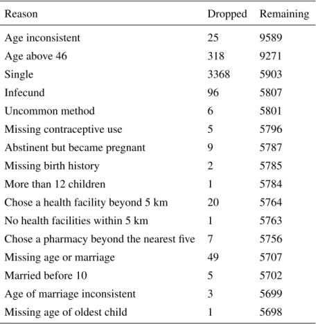
The baseline sample includes 9614 women between the ages of 15 and 49, of which 6927 were suc-cessfully interviewed at endline.4 The sample selection process is described in table 4.1 and starts with all 9614 women. At each step, I delete all person-year observations that do not meet the selection criterion. For example, if a woman is single at baseline and midterm but married at endline, I keep her endline observation.
3(Daff et al., 2014) describe in detail the IPM and how it resolved issues with the previous “pull-based” system, which relied on providers traveling to a local warehouse and using their own cash on hand to buy contraceptives.
4
Table 4.1: Sample Selection Process
Reason Dropped Remaining
Age inconsistent 25 9589
Age above 46 318 9271
Single 3368 5903
Infecund 96 5807
Uncommon method 6 5801
Missing contraceptive use 5 5796
Abstinent but became pregnant 9 5787
Missing birth history 2 5785
More than 12 children 1 5784
Chose a health facility beyond 5 km 20 5764
No health facilities within 5 km 1 5763
Chose a pharmacy beyond the nearest five 7 5756
Missing age or marriage 49 5707
Married before 10 5 5702
Age of marriage inconsistent 3 5699
25 women are dropped because their age is largely inconsistent across the two waves, and 318 are dropped because they are older than 46 at baseline (the last decision period in the model). There is limited sexual activity and contraceptive use outside of marriage in Senegal (4.5% of single women had sex in the past three months and merely 3.8% used contraceptives in the full baseline sample), therefore I limit the sample to married women. Most contraceptive users choose condoms, pills, injectables, implants or IUDs. A few women selected less common methods (sterilization, emergency contraception, spermicides, etc.) and are excluded from the sample. I also drop a small number of women who selected a health facility beyond 5 kilometers or a pharmacy beyond the nearest five.
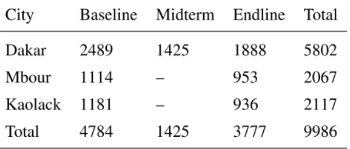
Table 4.2: Person-Year Observations City Baseline Midterm Endline Total
Dakar 2489 1425 1888 5802
Mbour 1114 – 953 2067
Kaolack 1181 – 936 2117
Total 4784 1425 3777 9986
The final sample is broken-down by city in table 4.2. There are 4784 observations at baseline, 1425 at midterm and 3777 at endline, for a total of 9986 person-year observations. 58.1% of these observations are in Dakar, 20.7% in Mbour and 21.2% in Kaolack.
Table 4.3: Provider Sample
Baseline Providers Endline Providers
City Health Facilities Pharmacies Health Facilities Pharmacies
Dakar 122 315 182 412
Mbour 13 27 19 27
Kaolack 25 32 27 34
Total 160 374 228 473
Gu´ediawaye, Pikine and Mbao, so I apply the endline supply environment to the midterm sample of women. Thus, I allow women to choose from the endline sample of providers in 2013.
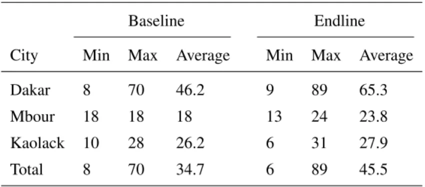
The size of the provider choice set varies by city and across women. The average choice set includes 34.7 providers at baseline and 45.5 providers at endline. The largest choice set includes 70 providers at baseline and 89 at endline. Note that there are always five pharmacies in a woman’s choice set, thus the largest choice set includes 84 health facilities plus 5 pharmacies.
Table 4.4: Provider Choice Set
Baseline Endline
City Min Max Average Min Max Average
Dakar 8 70 46.2 9 89 65.3
Mbour 18 18 18 13 24 23.8
Kaolack 10 28 26.2 6 31 27.9
Total 8 70 34.7 6 89 45.5
4.4. Model Variables
Table 4.5 provides summary statistics for the permanent characteristics of women in the estimation sample.eis the highest level of education at the age of marriage, categorized into none (0), primary (1), and secondary or more (2). The educational attainment of women is limited and typically doesn’t change after marriage, therefore it is treated it as a permanent characteristic of women in the model. 42.6% of women have no education, 36.4% have primary education, and merely 21.0% have secondary or more (I combine secondary and tertiary because only 3.6% of women have tertiary education).
ehis the husband’s level of education, which is defined in the same way ase. A larger share of husbands
I divide the age of marriage into three categories: before 18, between 18 and 23, and after 23. The majority of women (50.4%) get married between 18 and 23. Finally,χis equal to the number of health facilities that have a quality index greater than 0.65 and are located less than 2 kilometers from a woman baseline.
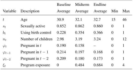
Table 4.5 provides summary statistics for the time-varying demographic variables in the estimation sample. A woman is considered sexually active if she had sex in the past three months. 85.2% of women are sexually active and 22.8% are using contraceptives at baseline. By endline, 36.6% of women are using contraceptives.
Table 4.5: Permanent Demographic Characteristics
Variable Description Average Min Max
I(e= 0) No education 0.426 0 1
I(e= 1) Primary education 0.364 0 1
I(e= 2) Secondary education 0.210 0 1
I(eh = 0) Husb. no education 0.473 0 1 I(eh = 1) Husb. primary education 0.207 0 1 I(eh = 2) Husb. secondary education 0.320 0 1
I(ω = 0) Poorest 0.355 0 1
I(ω = 1) Middle 0.337 0 1
I(ω = 2) Richest 0.308 0 1
a1 Married before 18 0.260 0 1
a2 Married between 18-23 0.504 0 1
a3 Married after 23 0.236 0 1
χ Baseline access 2.69 0 9
The average number of children increases from 2.98 at baseline to 3.24 at endline. Note that the endline sample includes women who were not married yet at baseline. Thus, the endline number of children is larger if one restricts the data to the matched baseline-endline sample (3.75 on average).
The timing of pregnancies is constructed by dividing the history of births into 12 month intervals. ϕt−2 = 1if a woman gave birth 12 to 23 months before the interview,ϕt−1 = 1if she gave birth 0 to 11 months before the interview, andϕt= 1if a child is born 1 to 12 months after the interview.
ξtis the number of ISSU community activities that a woman has been ever exposed to at timet, including
for all women at baseline. At endline, women have been exposed to 0.684 programs on average; 59.8% have not received any programs, 20.8% have received one, 12.0% have received two, 6.1% have received three, and 1.3% have received all four.
Table 4.6: Time-Varying Demographic Characteristics Baseline Midterm Endline
Variable Description Average Average Average Min Max
t Age 30.9 32.1 32.7 15 46
st Sexually active 0.852 0.862 0.860 0 1
bt Using birth control 0.228 0.354 0.366 0 1
nt Number of children 2.98 3.19 3.24 0 12
ϕt Pregnant int 0.190 0.158 – 0 1
ϕt−1 Pregnant int−1 0.214 0.197 0.168 0 1
ϕt−2 Pregnant int−2 0.209 0.180 0.173 0 1
ξt Program exposure 0 0.484 0.684 0 4
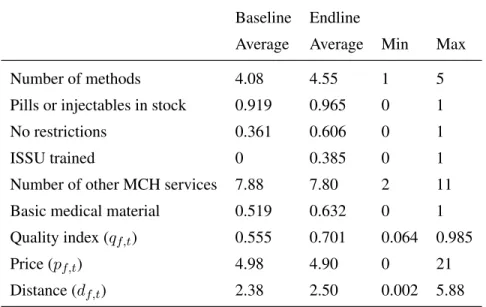
Table 4.7 provides summary statistics for the provider variables in the estimation sample. The quality index measures the quality of family planning services offered by health facilities (it is not defined for pharmacies). This index is an average of six quality indicators that are standard in the family planning literature and based on the Bruce framework (see section 2.2). The first indicator is the number of methods (condoms, pills, injectables, implants and IUDs) offered by the health facility at timet. The second is a dummy variable that is equal to one if pills and injectables (the most popular methods) are in stock at timet. The third quality indicator is the percentage of staff members (among those who offer reproductive health services) that do not impose any restrictions on contraceptives at timet. Restrictions include requiring women to have their husbands’ consent, to be within a certain age, or to have a minimum number of children in order to receive contraceptives. Together, these first three indicators capture the choice of methods in the Bruce framework. The fourth indicator is the percentage of family planning employees who received a training from ISSU at timet. The fifth indicator is the number of other MCH services that are offered at the health facility, which captures the constellation of services in the Bruce framework.5 The last indicator is a dummy variable that is equal to one if the health facility has all of the following basic medical material at timet: a
5
speculum, a tenaculum, a sponge clamp, antiseptics, cotton and gloves. I divide “number of methods” by 5 and “number of other MCH activities” by 11 to have indicators that range from 0 and 1, then I average the six indicators to obtain a quality index.
pf,tcaptures the average annual cost of obtaining contraceptives from providerfat timet. This variable
is based on the price of pills and injectables, which are the most popular methods in urban Senegal (see section 4.6). An injectable shot usually provides protection for 3 months and pills are sold in packs of 28. To obtain an annual cost, I set the price variable equal to(4×price of an injectable shot+ 12×price of a pack of pills)/2. Prices are expressed in thousands of CFA francs (1 dollar equals 500 CFA francs approximately).
Finally, the centroid of clusters and the exact location of providers were recorded by GPS, which allows me to compute the Euclidean distance from a woman’s dwelling place to each contraceptive provider.6 The largest value taken bydf tis 5.88 kilometers.
Table 4.7: Provider Variables Baseline Endline
Average Average Min Max
Number of methods 4.08 4.55 1 5
Pills or injectables in stock 0.919 0.965 0 1
No restrictions 0.361 0.606 0 1
ISSU trained 0 0.385 0 1
Number of other MCH services 7.88 7.80 2 11
Basic medical material 0.519 0.632 0 1
Quality index (qf,t) 0.555 0.701 0.064 0.985
Price (pf,t) 4.98 4.90 0 21
Distance (df,t) 2.38 2.50 0.002 5.88
4.5. Provider Choice
It can be seen in table 4.7 that the supply environment has improved between 2011 and 2015: the number of providers increased from 160 to 228, while the price of contraceptives declined slightly and the quality index increased on average. Figure 9.2 in the appendix provides the distribution of prices for public and
6
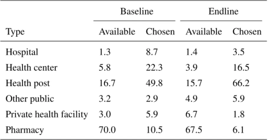
private providers. Public providers were cheaper on average in both waves. In addition, the government passed a decree in 2010 to set the price of contraceptives in the public sector, which resulted in a convergence of prices among public providers by 2015. Table 4.8 indicates that 83.6% of users in 2011 and 92.1% of users in 2015 obtained their method from a public provider. The most common choice is the health post, a relatively small and public health facility.
Table 4.8: Provider Types (%)
Baseline Endline
Type Available Chosen Available Chosen
Hospital 1.3 8.7 1.4 3.5
Health center 5.8 22.3 3.9 16.5
Health post 16.7 49.8 15.7 66.2
Other public 3.2 2.9 4.9 5.9
Private health facility 3.0 5.9 6.7 1.8
Pharmacy 70.0 10.5 67.5 6.1
Table 4.9 indicates that poorer women are more likely to choose providers that are cheaper and closer. Overall, the data suggests that distance is a significant determinant of provider choices. For example, client exit interviews reveal that 60.8% of women travelled by foot to their reproductive health appointments, 21.4% used public transportation, 13.7% employed taxis, 1.2% used a personal car, and 2.8% used a cart, motorcycle or other form of transportation in 2011.
Table 4.9: Provider Choice by Wealth Status
Baseline Endline Price (1000 CFA)
Poorest 1.768 1.375
Middle 1.938 1.353
Richest 2.111 1.684
All 1.943 1.460
Distance (km)
Poorest 0.979 0.836
Middle 1.080 0.944
Richest 1.078 1.032
All 1.048 0.935
Nearest (%)
Poorest 37.3 47.6
Middle 40.1 40.9
Richest 37.4 38.2
All 38.3 42.3
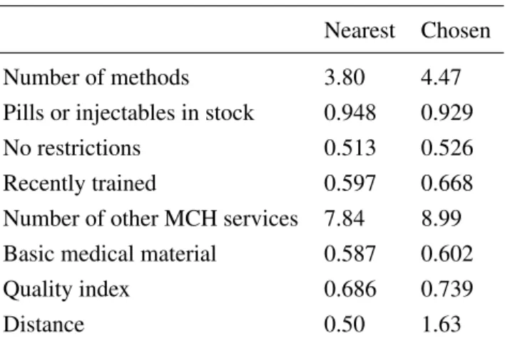
Table 4.10: Nearest vs. Chosen Provider in 2015 (Among Users Who Bypass)
Nearest Chosen
Number of methods 3.80 4.47
Pills or injectables in stock 0.948 0.929
No restrictions 0.513 0.526
Recently trained 0.597 0.668
Number of other MCH services 7.84 8.99 Basic medical material 0.587 0.602
Quality index 0.686 0.739
Distance 0.50 1.63
4.6. Reproductive Preferences
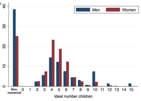
Figure 4.2: Fertility Preferences
Despite the low prevalence of contraceptives, most women desire to limit or space their pregnancies. 61.8% of married women report an ideal number of children between three and six at baseline (figure 7.1). 25.1% provide a non-numerical answer, such as “I do not know”, “I have not thought about it” or “it is up to God”. Among those who provide a numerical answer, the ideal family size is on average 5.0 children. Men tend to have stronger fertility preferences than women. 39.8% of married men report an ideal number of children between three and six at baseline, and 38.5% provide a non-numerical answer. Among those who provide a numerical answer, the ideal number of children is 6.0 on average. In terms of birth spacing, 91.4% of married women and 93.9% of married men prefer to have a two to four year interval between children (figure 4.3). Merely 0.4% of married women and 2.0% of married men want a birth interval shorter than two years.
Figure 4.3: Spacing Preferences
(22.3%), partner’s opposition (11.7%), personal opposition (11.2%), health issues (10.7%) and postpartum amenorrhea (10.2%). Note that there are widespread misconceptions about the harmfulness of contraceptives. For example, a significant share of women believe that people who use contraceptives end-up having health issues (57.5%) or that injectables cause irreversible sterility (32.2%) at baseline.
Table 4.11: Communication With Husband and Agency Over Reproductive Decisions at Baseline (%)
Yes No You Joint Husb. Other1 Ever talked about number
of children with husband 30.1 69.9
Ever talked about FP with husband 54.8 45.2 Need husband’s consent to use FP 80.6 19.4 Can convince husband to use FP 79.9 20.1
Who decides num. of children mainly 24.2 32.1 14.4 29.3
Who chooses the method mainly 51.2 34.1 8.1 6.6
1
SECTION 5
REDUCED-FORM ANALYSIS
I employ a fixed-effects model to evaluate the impact of the awareness campaign on contraceptive use and to explore various impact mechanisms. The structural model expresses the decision to use contraceptives as a function of a woman’s age, number of children (interacted with education and husband’s education), time since last pregnancy, program exposure, the supply environment and several time invariant variables (education, husband’s education, baseline wealth status, age of marriage and baseline access to quality). I exclude the supply environment from my reduced-form model and drop the time invariant variables:
bt=λ0+λ1t+λ2t2+nt
X2
k=1
λ3,kI(e=k) +
2
X
k=1
λ4,kI(eh=k)
+n2t
X2
k=1
λ5,kI(e=k) +
2
X
k=1
λ6,kI(eh=k)
+λ7ϕt−1+λ8(1−ϕt−1)ϕt−2
+λ9ξt+ν+t (5.1)
wheretis a woman’s age,eher level of education,eh her husband’s education,ϕt−1 her pregnancy status one year ago,ϕt−2her pregnancy status two years ago, andν is an individual fixed-effect. I estimate this model with fixed effects, using the sample of women who have at least two observations (3391 women). This model is relatively simple and static, but it controls for permanent unobserved heterogeneity. Essentially, the model captures the change in contraceptive use that is associated with program exposure by controlling for the baseline level of contraceptive use.
significant impact on contraceptive use (table 5.1). The radio coefficient is positive but not significant at the 10% level (pvalue = 0.18). In contrast, the parameter associated with the community variable is significant at the 1% level and is equal to 0.046, which implies that the probability of using contraceptives increases by 4.6 percentage points with each additional community program that a woman receives. Simulations suggest that exposing all women to the four community activities at endline would increase contraceptive use from 39.4% to 55.6%. In addition, this model fits well the average level of contraceptive use at baseline (25.8%) and endline (39.4%) in the matched sample.
I exclude the radio and television variables in the second model and obtain the same results. Since radio and television do not have a significant impact on the decision to use contraceptives, I only include the community variable in my structural model. This reduces the computation burden of the model—including radio and television would add two more probability of exposure equations, one for each type of program.
Table 5.1: Impact of Different Family Planning Programs
Model 1 Model 2
Radio 0.030
(0.019)
Television -0.014
(0.017)
Community 0.050∗∗∗ 0.052∗∗∗
(0.010) (0.096)
Controls Yes Yes
Fixed effects Yes Yes
R2 0.0529 0.0529
Model fit
Data 2011 0.253 0.253
Model 2011 0.264 0.263
Data 2015 0.391 0.391
Model 2015 0.390 0.390
Counterfactual (community=4)
Model 2015 0.570 0.558
Number of observations 3391 3391
Standard errors are clustered at the cluster level (in parenthesis).
∗∗∗
Significant at the 1% level.
∗∗
Significant at the 5% level.
∗
SECTION 6
STRUCTURAL ESTIMATION
6.1. Likelihood Function
Given a vector of parametersθ, the likelihood function for womaniconditional on her typeµis:
Li(θ|µ) =Y t
Y
j
pj(Ωit, θ, µ)Pj(Ωit, θ, µ)ϕit(1−Pj(Ωit, θ, µ))(1−ϕit)
dijt
×φ(ξit|Ωit, θ, µ)
wheredijtis a dummy that is equal to one if individualichoosesjat timetandφis the probability
density function of ξit ∼ N(0, σ2) . The likelihood of the observed data is a weighted average of the
type-specific likelihood functions, multiplied across individuals:
L(θ) =Y i
L
X
l=0
P(µ=l)Li(θ|µ=k)
θis estimated by maximizing the likelihood function with a Quasi-Newton algorithm. At each iteration, a line search is performed in a direction determined by the negative inverse Hessian times the gradient of
L, where the Hessian is approximated using the Broyden, Fletcher, Goldfar, and Shanno (BFGS) method. Standard errors are computed by estimating the asymptotic covariance matrix of the maximum likelihood estimator with the Outer Product of the Gradient (OPG) method.
6.2. Identification
the effect of the supply environment and family planning programs in the utility function. There are two potential sources of endogeneity that must be addressed in this regard.
First, access to quality might be correlated with the unobserved determinants of contraceptive use for various reasons discussed in section 2.1. To illustrate this point, suppose there are two types of women. Type one is less likely to use contraceptives due to some fixed unobservable characteristics. In addition, type one is more present in underserved areas where provider quality is generally lower. In this case, there is a spurious positive correlation between contraceptive use and access to quality. As discussed in the literature review, the common approach of aggregating quality at the cluster level, controlling for a limited number of community variables, would bias results.
In contrast, my model controls for permanent unobserved differences in the disutility of contraceptives (such as personal opposition) and in fertility preferences (such as a stronger taste for children) with a discrete number of unobserved types. Access to quality determines the unobserved type of a woman, which shifts her fertility and contraceptive preferences in the utility function. This allows for a correlation between access to quality and the unobserved determinants of fertility and contraceptive preferences.
SECTION 7
RESULTS
7.1. Parameter Estimates
Table 9.1 (appendix) reports the estimates and standard errors of the parameters in the utility function. The model is fit with three types. Type one women have a larger disutility of using contraceptives (-1.834) than type zero (-1.356) and type two (-1.506) women. As expected, the parameters associated with price (α6, α7) and distance (α8, α9) are negative and larger for poorer women, while the parameters associated with provider quality (α5) and family planning programs (α10) are both positive. Note thatα4is equal to -0.258 andα5is equal to 0.738. Thus, between a health facility and an equally distant and priced pharmacy, a woman will prefer the health facility if its quality index is greater than0.258/0.738 = 0.3501. Parameters α11throughα18indicate that type one women have lower fertility preferences compared to type zero and type two women and that education reduces fertility preferences (see figure 7.1). The cost of pregnancy increases with age and if a woman gave birth recently. Finally,ρis equal to 0.252, indicating that provider choices are correlated, and the discount factor is fixed at 0.9.2
Table 9.3 (appendix) reports the estimates and standard errors of the parameters in the pregnancy equation. The probability of pregnancy decreases with age, if a woman gave birth in the last period, and if she uses birth control. In addition, type one and two women are less likely to become pregnant, conditional on being sexually active.
Table 9.2 (appendix) provides the estimates of the exposure equation. Exposure increased significantly in 2015 compared to 2013. Type one women were the most likely to be exposed to the community programs, followed by type zero women. In addition, older women were slightly more likely to receive the intervention (β5is significant at the 10% level), but exposure did not vary significantly by education and wealth status.
1
Just 5.0% of health facilities have a quality index below 0.350 at baseline
Figure 7.1: Fertility Preferences by Education (Type 1)
Table 7.1: Permanent Characteristics by Simulated Type
Type 0 Type 1 Type 2
No education 44.8 38.8 42.3
Primary 36.8 42.3 35.7
Secondary 18.4 18.9 21.9
Husb. no education 50.2 48.4 45.7
Husb. primary 19.5 20.4 20.3
Husb. secondary 30.3 31.3 34.0
Poorest 39.3 40.4 34.0
Middle 36.4 35.1 32.8
Richest 24.3 24.5 33.2
Married before 18 26.9 28.0 25.5
Married between 18-23 55.5 53.7 48.7
Married after 23 17.5 18.3 25.8
Access 2.6 2.5 2.7
Sample percentage 20.9 6.6 72.6
Table 9.4 (appendix) provides the parameter estimates of the type equation, with type zero parameters normalized to zero. In addition, Table 7.1 shows the average characteristics of women by simulated type, where types are drawn 200 times for each woman. Type zero, one and two represent 20.9%, 6.6% and 72.6% of the sample respectively. Type zero and type one have similar permanent characteristics, except that type zero is more likely to have no education and type one is more likely to have primary education. Type two, which is unlikely to receive the intervention, tends to be more educated, have more educated husbands, be more wealthy, get married latter and have slightly better access to quality than the two other types.
Table 7.2 is derived by drawing types 200 times for each women. I then simulate choices, pregnancies and program exposure conditional on a woman’s observed state variables at baseline, midterm and endline. I report the percentage of women that that make each choice and the percentage that become pregnant in the pooled sample, by type. I also provide the average level of exposure at midterm and endline by type.
Table 7.2: Choices, Pregnancies and Exposure by Simulated Type
Type 0 Type 1 Type 2
No sex 11.9 15.5 14.9
Unprotected sex 58.5 61.0 54.5
Protected sex 29.5 23.5 30.6
Pregnant 19.0 15.9 16.9
Midterm exposure 1.3 2.8 -0.1
Endline exposure 1.5 3.1 0.2
Sample percentage 20.9 6.6 72.6 All variables are expressed in percentage, except for Midterm
exposure and Endline exposure.
7.2. Model Fit
Figure 7.2 shows the percentage of women who choose to be abstinent, have protected sex or unprotected sex in the data (solid lines) and the simulated sample (dashed lines), averaged over two-year age bins.3 The model fits the data well. Contraceptive use is low at younger ages and increases over the life cycle. This pattern is consistent with the parameter estimates, which imply that the cost of pregnancy increases with age and the marginal utility of children decreases with parity. On the other hand, the probability of pregnancy declines with age (figure 7.3), which explains the uptake of unprotected sex towards the end of the reproductive life cycle.
Figure 7.2: Choices
Figure 7.3: Pregnancies at Baseline
The percentage of pregnant women decreases over the life cycle and is lower among those who use birth control (appendix figure 9.3). In addition, women are less likely to become pregnant if they gave birth recently. This can be seen in table 9.5 in the appendix for women under the age of 30.4
Table 7.3 shows that women with primary or secondary education are more likely to use contraceptives or be abstinent compared to women with no education. In addition, the model fits well the characteristics of the providers chosen by women (table 7.4) and the level of program exposure at midterm and endline (table 7.5). Finally, exposure is correlated with greater contraceptive use at midterm and endline (table 7.6).
4
Table 7.3: Choices by Education (%) Data Model No education
Abstinence 13.3 13.4
Unprotected sex 61.2 60.4 Protected sex 25.5 26.2 Primary
Abstinence 14.5 15.1
Unprotected sex 52.1 52.9 Protected sex 33.4 32.0 Secondary
Abstinence 16.5 15.0
Unprotected sex 51.1 51.0 Protected sex 32.5 34.0
Table 7.4: Provider Choices (%) Data Model Chosen quality 0.691 0.680 Chosen distance 0.983 0.997 Chosen price 1.664 1.682
Table 7.6: Contraceptive Use by Exposure at Midterm and Endline (%)
Data Model Not exposed (ξt= 0) 32.1 29.0
Exposed (ξt>0) 43.2 43.9
SECTION 8
POLICY EXPERIMENTS
The estimated model allows me to simulate choices and pregnancies over the reproductive life of women, under different types of scenarios. I start by decomposing the increase in contraceptive use that occurred between 2011 and 2015 into three factors: women progressing through their life cycle (i.e. aging and having children), changes to the supply environment, and exposure to family planning programs. I use the sample of women who have both a baseline and an endline observation for this simulation exercise. The first line of table 8.1 shows the percentage of contraceptive users in the matched sample in 2011. Next, I simulate choices 200 times for each woman, conditional on her observed state variables in 2011. The model predicts that 25.21% of women use contraceptives at baseline. I then fix the supply and exposure variables to their baseline values and simulate choices and pregnancies from 2011 to 2015. In this simulation, the environment is kept constant and women are aging, which isolates the effect of the first factor. The next simulation is similar, except that I update all the provider variables to their endline values in 2013.1 Exposure variables are kept to their baseline values (zero) in order to isolate the effect of the second factor. In the last simulation, I update both the provider and exposure variables in 2013.
Table 8.1: Effect Decomposition (%) Users
Baseline data 25.77
Baseline simulation 25.21
Fixed environment 25.54
Supply change 29.48
Supply change and exposure 35.56
Endline data 39.37