Eckert_unc_0153D_16293.pdf

(1)

A MASS CENSUS OF THE NEARBY UNIVERSE WITH THE RESOLVE SURVEY

Kathleen Eckert

A dissertation submitted to the faculty at the University of North Carolina at Chapel Hill in partial fulfillment of the requirements for the degree of Doctor of Philosophy in the Department

of Physics and Astronomy.

Chapel Hill 2016

Approved by:

Sheila Kannappan

Andreas Berlind

Arthur Champagne

J. Christopher Clemens

(2)

(3)

ABSTRACT

Kathleen Eckert: A Mass Census of the Nearby Universe with the RESOLVE Survey (Under the direction of Sheila Kannappan)

The galaxy mass function, i.e., the distribution of galaxies as a function of mass, is a useful way to characterize the galaxy population. In this work, we examine the stellar and baryonic mass function, and the velocity function of galaxies and galaxy groups for two volume-limited surveys of the nearby universe. Stellar masses are estimated from multi-band photometry, and we add cold atomic gas from measurements and a newly calibrated estimator to obtain baryonic mass. Velocities are measured from the internal motions of galaxies and groups and account for all matter within the system. We compare our observed mass and velocity functions with the halo mass function from theoretical simulations of dark matter, which predict a much more steeply rising low-mass slope than is normally observed for the galaxy mass function.

We show that taking into account the cold gas mass, which dominates the directly detectable mass of mass galaxies, steepens the mass slope of the galaxy mass function. The low-mass slope of the baryonic low-mass function, however, is still much shallower than that of the halo mass function. The discrepancy in low-mass slope persists when examining the velocity function, which accounts for all matter in galaxies (detectable or not), suggesting that some mechanism must reduce the mass in halos or destroy them completely. We investigate the role of environment by performing group finding and examining the mass and velocity functions as a function of group halo mass. Broken down by halo mass regime, we find dips and varying low-mass slopes in the mass and velocity functions, suggesting that group formation processes such as merging and stripping, which destroy and lower the mass of low-mass satellites respectively, potentially contribute to the discrepancy in low-mass slope.

In particular, we focus on the nascent group regime, groups of mass ∼1011.4−12 _M _{with few}

(4)

(5)

ACKNOWLEDGEMENTS

The work presented in this thesis was performed with the advice, help, and support of many people. First, I would like to thank my advisor, Sheila Kannappan, for providing me the opportunity to become a leader within the RESOLVE survey team. With Sheila’s support and guidance, I have been able to explore many facets of astronomy including instrumentation, astrostatistics, and radio and optical observing. I also thank Sheila for helping me to become a better writer, an experienced observer and programmer, and a mentor to younger students.

I would also like to thank the members of my thesis committee: Andreas Berlind, Art Cham-pagne, Chris Clemens, and Adrienne Erickcek. Their useful advice, guidance, and insightful ques-tions have contributed greatly to this work and my development as a researcher. I would especially like to thank Chris Clemens and Andreas Berlind for their mentorship in instrumentation and scientific pursuits respectively.

I am grateful to the RESOLVE team, who have contributed to this work in innumerable ways. In particular, I wish to acknowledge Amanda Moffett, David Stark, Mark Norris, Elaine Snyder, Kirsten Hall, Ashley Baker, Ashley Bittner, and Erik Hoversten, who have provided key data, analysis tools, and a sounding board for ideas (both brilliant and wacky), and who have made this journey a fun and collaborative experience.

I also want to thank my undergraduate advisor, Mark Devlin, for providing me my first intro-duction to astronomical instrumentation and advising my senior thesis project, which encouraged me to continue doing research in astronomy.

I acknowledge the funding that has supported me throughout my completion of this thesis: NSF grants AST-0955368 and OCI-1156614, the UNC Board of Governor’s Fellowship in Science and Technology, Graduate Assistance in Areas of National Need, Sigma Xi Grant-in-Aid of Research, the North Carolina Space Grant, and the UNC Royster Society Dissertation Completion Fellowship (funded by Lovick P. Corn).

(6)

(7)

PREFACE

Images of galaxies have long captured the imagination of astronomers and the public alike. These beautiful pictures, however, reveal only one facet of galaxies – the contribution from stars like our sun. Galaxies consist of several other components that can be directly observed (at wavelengths outside the visible spectrum) such as gas, the raw material for star formation. Most puzzling, however, is the dark matter revealed indirectly from studying the motions of galaxies and that has so far eluded direct detection. In this thesis we examine the link between galaxies and dark matter by studying galaxy mass content through stars, stars+gas, and total mass from internal motions and by comparing with simulations of dark matter.

The first project of this thesis (Chapter 2) has been published in The Astrophysical Journal

(8)

(9)

TABLE OF CONTENTS

LIST OF TABLES . . . xv

LIST OF FIGURES . . . xvi

LIST OF ABBREVIATIONS AND SYMBOLS . . . xx

1 Introduction . . . 1

1.1 Background . . . 1

1.2 Methods & Data Sets . . . 4

1.3 Results Summary . . . 5

2 RESOLVE Survey Photometry and Volume-limited Calibration of the Photo-metric Gas Fractions Technique . . . 8

2.1 Introduction . . . 8

2.2 Data Sets . . . 12

2.2.1 RESOLVE-A . . . 14

2.2.2 RESOLVE-B . . . 15

2.3 Data . . . 15

2.3.1 Photometric Data . . . 16

Custom Processed Data . . . 17

Magnitude Extrapolation . . . 21

Comparison with Catalog Photometry . . . 27

2.3.2 Stellar Masses . . . 32

(10)

2.4 Color-limited PGF Calibrations . . . 37

2.5 Correlations with 3rd Parameters . . . 40

2.5.1 Best 3rd Parameter for Gas Mass Estimation . . . 40

2.5.2 Physical Drivers of Residual Correlations . . . 44

2.5.3 Modified Color-Limited PGF Calibration . . . 48

2.6 Probability Density Field PGF Calibrations . . . 49

2.6.1 Calibration Description . . . 50

2.6.2 Reinserting the Missing Galaxies . . . 52

2.6.3 How to Use the PGF Calibration . . . 54

2.6.4 Adding in High M_bary/L Galaxies . . . 56

2.7 Discussion . . . 58

2.8 Conclusions . . . 63

3 RESOLVE and ECO: The Halo Mass-Dependent Shape of Galaxy Stellar and Baryonic Mass Functions . . . 66

3.2 Data Sets . . . 70

3.2.1 Common Features of RESOLVE and ECO . . . 71

3.2.2 RESOLVE-B . . . 72

3.2.3 ECO . . . 74

3.2.4 Densities of RESOLVE-B and ECO . . . 76

3.3 Data And Methods . . . 77

3.3.1 Photometric Data . . . 78

3.3.2 Stellar Masses . . . 79

(11)

RESOLVE-B Gas Inventory . . . 81

ECO Gas Inventory . . . 83

Estimating Gas Masses . . . 83

3.3.4 Baryonic Masses . . . 84

Choice of PGF Estimator . . . 85

Calculation of Baryonic Masses . . . 86

3.3.5 Group Identification and Halo Masses . . . 88

Choice of Linking Lengths . . . 88

Group Finding and Halo Mass Assignment . . . 89

3.3.6 Completeness of Data Sets . . . 94

RESOLVE-B Completeness . . . 94

ECO Completeness Corrections . . . 96

Stellar and Baryonic Mass Completeness . . . 99

3.4 Statistical Analysis of Stellar and Baryonic Mass Functions . . . 101

3.5 Stellar and Baryonic Mass Functions . . . 104

3.5.1 Choice of Stellar Population Models . . . 106

3.5.2 Overall SMF and BMF . . . 106

Mass Function Fit Parameters . . . 107

The SMF . . . 108

The BMF . . . 111

Divergence of SMF & BMF . . . 112

Relationship of Observed Galaxy to Theoretical HMFs . . . 114

3.5.3 Conditional SMF and BMF . . . 114

(12)

SMF and BMF by Group Halo Mass (“Conditional Mass Functions”) . . . . 116

Central Galaxy Mass Functions in Each Group Halo Mass Bin . . . 119

Satellite Galaxy Mass Functions in Each Group Halo Mass Bin . . . 121

Comparison to Previous Work . . . 122

Mass Function Reconstruction . . . 124

3.6.1 How Group Halo Mass Environment Shapes the Galaxy Mass Function . . . 127

3.6.2 Comparison Between Galaxy and Halo Mass Functions . . . 128

4 The Baryonic Collapse Efficiency in Galaxy Groups in the RESOLVE and ECO surveys . . . .134

4.2 Data And Methods . . . 135

4.2.1 Data Sets . . . 136

4.2.2 Photometry & Galaxy Stellar and Cold Baryonic Masses . . . 138

4.2.3 Group Stellar, Cold Baryonic, and Halo Masses . . . 139

Group-Integrated Stellar and Cold Baryonic Mass . . . 140

Group Halo Abundance Matching . . . 141

Group Dynamical Masses . . . 141

Group Dynamical Masses Through Stacking . . . 143

Final Dynamical Group Mass Estimates . . . 145

4.2.4 The Semi-analytic Model Mock Catalog . . . 147

4.3 Group Mass Functions and Baryon Fractions . . . 149

(13)

4.3.2 Group Stellar & Cold Baryon Fractions . . . 153

4.3.3 Adding The Hot Gas . . . 160

4.4.1 Baryonic Collapse Efficiency and Galaxy Formation Efficiency: From Isolated Dwarfs to Nascent Groups . . . 162

4.4.2 Undetected Gas . . . 164

4.4.3 HAM vs. Dynamical Group Mass . . . 166

5 A Preliminary Velocity Function for the RESOLVE survey and its Dependence on Environment . . . .170

5.2 RESOLVE-B . . . 172

5.3 Kinematic Data . . . 175

5.3.1 Kinematic Setups . . . 175

Emission Line Setup . . . 176

Absorption Line Setup . . . 177

HI Data . . . 178

5.3.2 Data Reduction . . . 179

5.3.3 Velocity Extraction . . . 180

Rotation Velocities . . . 180

HI Velocity Width Calibration . . . 185

Velocity Dispersions . . . 186

5.4 Results . . . 187

5.4.1 Mass-Velocity Relation . . . 188

(14)

Comparison to Simulations . . . 193

The VF as a function of Group Halo Mass . . . 194

6 Conclusions and Future Work . . . .200

(15)

LIST OF TABLES

2.1 RESOLVE Custom Photometry Catalog Description . . . 24

2.2 Color-limited Photometric Gas Fraction Calibrations . . . 39

2.3 Modified Color-limited Photometric Gas Fraction Calibrations . . . 49

2.4 Full-Probability Photometric Gas Fractions Calibrations for Color Only . . . 55

2.5 Full-Probability Photometric Gas Fractions Calibrations for Modified Color . . . 55

2.6 Full-Probability Photometric Gas Fractions Calibrations for Color Only Including High M_bary/L Galaxies . . . 57

2.7 Full-Probability Photometric Gas Fractions Calibrations for Modified Color Including High M_bary/L Galaxies . . . 57

3.1 Central Stellar and Baryonic Mass to Group Halo Mass Fit Parameters . . . 92

3.2 All RESOLVE-B and ECO Stellar and Baryonic Mass Functions . . . 104

3.3 Single and Double Schechter Function Parameters for RESOLVE-B and ECO stellar and baryonic mass functions . . . 108

4.1 Fitting Parameters for Group-Integrated Mass Function . . . 151

(16)

LIST OF FIGURES

2.1 RA–cz plot of RESOLVE-A and -B semesters . . . 13

2.2 Absolute r-band magnitude distribution of RESOLVE-A and -B subvolumes . . . . 14

2.3 Illustration of the three methods for extrapolating total magnitudes . . . 22

2.4 Comparison of newly reprocessed photometry and SDSS DR7 photometry . . . 28

2.5 Comparison of our newly reprocessed colors and SDSS DR7 model colors . . . 30

2.6 Comparison of photometric measurements for galaxies in both RESOLVE and ECO . . 31

2.7 Color vs. stellar mass for the entire RESOLVE survey . . . 34

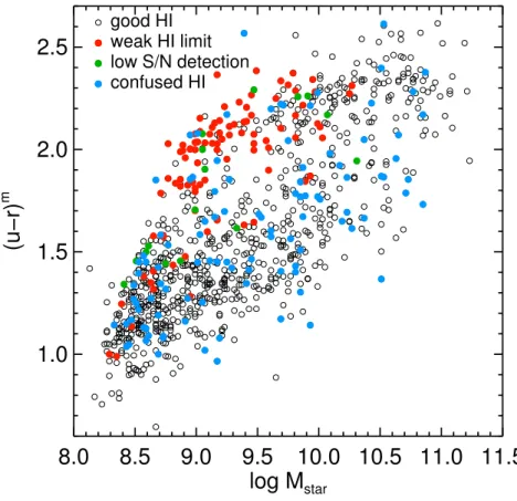
2.8 Color vs. stellar mass relationship for the RESOLVE-A data set color coded by HI quality 37 2.9 Photometric gas fractions relation foru−J SED modeled color . . . 39

2.10 Residuals in log(G/S) from the PGF calibration for (u−J)m plotted against various photometric parameters . . . 42

2.11 Residuals in log(G/S) shown as a function of galaxy morphological type and µr,50,b/a, and stellar mass corrected ∆g−r . . . 46

2.12 Test of the effect of dust on the relationships between log(G/S), color, and axial ratio . 47 2.13 Log(G/S) vs. modified (u−J)m color for RESOLVE-A. . . 51

2.14 Best fit model to the PGF density field using modified (u−J)m color . . . 54

2.15 Probability distributions of log(G/S) for three modified (u−J)m colors . . . 56

2.16 Comparison of PGF calibrations from this work and the literature using 21cm data for RESOLVE-B . . . 62

3.1 RA–cz distribution for the Stripe 82 subvolume of RESOLVE . . . 72

3.2 Luminosity distributions for the Stripe 82 subvolume of RESOLVE . . . 73

(17)

3.5 Frequency distributions of group integratedr-band luminosity and relationship between

group luminosity and group mass . . . 90

3.6 Group halo mass distributions for RESOLVE-B and ECO . . . 91

3.7 Relationship between galaxy stellar or baryonic mass and group halo mass . . . 93

3.8 Evaluation of the extra completeness of RESOLVE-B due to redshift completion as a function of surface brightness . . . 95

3.9 Relative frequencies ofr-band absolute magnitude for the original and final RESOLVE-B data sets and the raw and completeness-corrected ECO data sets . . . 97

3.10 Determination of stellar and baryonic mass completeness limits for ECO and RESOLVE-B100 3.11 RESOLVE-B SMF calculated two different ways . . . 103

3.12 RESOLVE-B and ECO SMFs and BMFs and comparison to previous work . . . 110

3.13 RESOLVE-B and ECO SMFs and BMFs with single and double Schechter function fits . 111 3.14 Direct comparison of the RESOLVE-B and ECO SMF and BMF . . . 113

3.15 Breakdown of RESOLVE-B and ECO SMF and BMF into different group halo mass regimes . . . 117

3.16 RESOLVE-B SMF and BMF broken down by group halo mass regime and central vs. satellite designation . . . 119

3.17 ECO SMF and BMF broken down by group halo mass regime and central vs. satellite designation . . . 120

3.18 Reconstruction of the RESOLVE-B BMF using the ECO conditional mass functions . . 126

4.1 Group-integrated cold baryonic mass vs. group halo mass measured by HAM and dy-namical estimates . . . 143

4.2 Residual correlations between ∆logM_halo and various group photometric properties . . . 144

4.3 Method to determine the scale factor A(σ) for estimating dynamical mass . . . 146

4.4 Comparison of HAM and dynamical group mass estimates . . . 147

4.5 Group SMF and CBMF for ECO and RESOLVE-B . . . 150

(18)

4.7 Conditional density plot of group-integrated stellar and cold baryon fraction as a function

of HAM group halo mass . . . 154

4.8 Conditional density plot of group-integrated stellar and cold baryon fraction as a function of HAM group halo mass (using stellar mass) . . . 155

4.9 Conditional density plot of group-integrated stellar and cold baryon fraction as a function of dynamical group halo mass . . . 156

4.10 Conditional density plot of group-integrated stellar and cold baryon fraction for the SAM FOF groups . . . 157

4.11 Conditional density plot of group-integrated stellar and cold baryon fraction for the SAM FOF groups with stellar mass based HAM . . . 158

4.12 Conditional density plot of group-integrated stellar and cold baryon fractions for the SAM true groups . . . 159

4.13 Conditional density plot of the ratio of hot halo gas to collapsed galaxy gas mass for SAM true groups . . . 160

4.14 The group BMF including hot halo gas . . . 161

4.15 The group BMF including hot halo gas and potentially undetected gas . . . 165

5.1 Characteristics of the RESOLVE-B data set . . . 173

5.2 Frequency distributions of size, axial ratio, and morphology for RESOLVE-B galaxies . . 174

5.3 Velocity field and Vpmm determination for RESOLVE-B galaxy rf0294 . . . 184

5.4 Comparison between kinematic and photometric inclinations and between 2D and 1D Vpmm measurements . . . 185

5.5 Comparison between optical rotation curve and radio velocity width measurements . . . 186

5.6 Galaxy mass-velocity relation . . . 188

5.7 Mass-velocity relation with truncated and asymmetric rotation curves highlighted . . . . 190

5.8 The RESOLVE-B VF and comparison to previous work . . . 191

5.9 RESOLVE-B VF compared with the halo circular VF from simulations . . . 193

(19)

(20)

LIST OF ABBREVIATIONS AND SYMBOLS

2MASS Two Micron All Sky Survey AAT Anglo-Australian Telescope

ALFALFA The Arecibo Legacy Fast ALFA Survey b/a axial ratio

BMF baryonic mass function CBMF cold baryonic mass function Cr Concentation index (R90/R50)

CSP composit stellar population ∆g−r g−r color gradient

Dec Declination

E15 Eckert et al. (2015) E16 Eckert et al. (2016) ECO Environmental COntext FOF Friends-of-Friends

GALEX The Galaxy Evolution Explorer GASS Galex Arecibo SDSS Survey G/S gas-to-stellar mass ratio HI 21cm atomic hydrogen gas HAM halo abundance matching HMF halo mass function

HOD halo occupation distribution IMF initial mass function

(21)

M15 Moffett et al. (2015)

M solar mass

mc modified color M_HI atomic gas mass Mcold_bary cold baryonic mass M_bary baryonic mass

Mgas 1.4×atomic gas mass

M_star stellar mass

Mr,tot r-band absolute magnitude

N Number of group members

µr,50 r-band surface brightness within the half-light radius

µr,90 r-band surface brightness within the 90%-light radius

PA position angle

PGF photometric gas fractions R50,r half-light radius inr-band

R90,r 90%-light radius inr-band

RESOLVE REsolved Spectroscopy of a Local VolumE RA Right Ascension

NFGS Nearby Field Galaxy Survey SAM semi-analytic model

SED spectral energy distribution SDSS Sloan Digital Sky Survey SMF stellar mass function

(22)

SSP simple stellar population S/N signal to noise ratio T galaxy morphological type

UKIDSS UKIRT InfraRed Deep Sky Survey UVOT Ultraviolet/Optical Telescope VDF velocity dispersion function VF velocity function

Vpmm probable min-max velocity

W50 HI velocity width

z redshift

(23)

CHAPTER 1: Introduction

1.1 Background

Galaxies such as our Milky Way consist of stars, which are directly observed through ultraviolet, optical, and infrared light. Additionally, galaxies are composed of gas, the raw material for star formation that is directly observed through radio emission. The galaxy stellar and gas mass is referred to as “baryonic,” which means it consists of normal matter like the atoms that make up the world we know. Measurements of galaxy internal motions, however, reveal that galaxies are much more massive than their stars and gas would indicate (e.g., Rubin 1983). This inferred extra component, referred to as “dark matter” cannot be directly observed at any wavelength of light. Typically, dark matter is assumed to be an exotic form of matter, i.e., non-baryonic. It may, however, also contain an undetected baryonic component in the form of either ionized gas or ultra cold molecular hydrogen gas.

Through a combination of observations of the distribution of galaxies in space (e.g., the 2DF galaxy redshift survey, Colless et al. 2001) and N-body simulations of non-baryonic dark matter (e.g., the Millennium simulation, Springel et al. 2005), a powerful theory of galaxy evolution has emerged. Galaxies form inside halos of dark matter, which extend much farther than the visible size of the galaxy. Over time, the galaxies (and their dark matter halos) interact and merge in a hierarchical manner, forming larger structures such as groups and clusters of galaxies in shared halos, as well as filaments, walls, and voids, where few galaxies reside. Thus galaxies and dark matter halos are linked in their growth and evolution.

(24)

estimate stellar masses, are readily available for large surveys. In mathematical terms the stellar mass function exhibits a power law slope that rises towards lower masses, with typical values ranging from −1.0 to −1.2 (Cole et al. 2001; Blanton et al. 2003b; Bell et al. 2003b; Panter et al. 2007; Li & White 2009). Dark matter simulations yield similarly shaped halo mass functions; however, the low-mass slope of the dark matter halo mass function is significantly steeper, with a slope of ∼−2.0 (Sheth & Tormen 1999). The discrepancy between low-mass slopes raises the question:

why do we not observe as many galaxies as predicted by cold dark matter simulations? To answer this question, we consider three possible explanations for the discrepancy: dark baryons, depressed baryon-fraction halos, and the role of environment.

Dark Baryons: From observations of primordial fluctuations in the early universe, we expect the baryon-to-dark matter ratio to be ∼0.15 (Planck Collaboration et al. 2014). In studies of galaxies and galaxy groups, however, we generally cannot account for most of these baryons via stars and gas alone (up to 99% are unaccounted for in low-mass galaxies, McGaugh et al. 2010). For the largest clusters the shortfall is within systematic uncertainties on observable quantities when including the hot X-ray detected gas (Gonzalez et al. 2007; Giodini et al. 2009). For lower mass groups, however, the gas is not as hot and does not emit in X-rays, leaving us unable to easily detect the remaining baryons, most of which are expected to be in the form of the warm-hot intergalactic medium or WHIM (40–50% based on simulations, Cen & Ostriker 2006). In fact, a massive reservoir of ionized gas has been detected in the Milky Way using quasar absorption line studies (Gupta et al. 2012). There is also evidence for dark baryons in disks in the form of ultra-cold gas, as revealed by submillimeter excesses in low-mass galaxies (R´emy-Ruyer et al. 2013). If there is a large reservoir of undetected baryonic matter in the galaxy disk, galaxy mass functions based on detectable baryons (such as stellar mass) will underestimate the mass of galaxies, leading to the shallower low-mass slope in the observed galaxy mass function.

(25)

star formation (Mac Low & Ferrara 1999) and 2) early reionization of the neutral gas after the first stars formed in the universe (Thoul & Weinberg 1996), “squelching” galaxy formation in low-mass halos thereafter (Tully et al. 2002). Supernova winds are efficient at removing gas only for the lowest mass galaxies (Mstar <107M, Mac Low & Ferrara 1999), although they may remove some

of the gas in galaxies with gas masses of∼109 _M_{(Ferrara & Tolstoy 2000) thereby depressing the}

baryon fraction within these halos. Reionization provides a better mechanism for fully suppressing star formation in low-mass halos. However, detailed examination of the star formation history of dwarf galaxies shows that dwarfs have continued to form stars since the epoch of reionization (Monelli et al. 2010), suggesting that reionization does not completely shut down galaxy formation in low-mass halos. Additionally we lack strong evidence for a large population of dark halos as would be expected if most of the discrepancy can be explained by a galaxy formation inefficiency scenario (see Cannon et al. 2015 and references therein). A less severe option is that part but not all of the baryonic material in the halo is removed, resulting in high mass-to-light ratio halos. Such baryon depletion may be accomplished by reionization or partial supernova blowout of galaxy gas or possibly environmental effects as discussed below. If a complete accounting for the baryons in galaxies still results in a divergence between observed and theoretical low-mass slopes, then a mechanism to reduce the baryon fraction in halos needs explanation.

(26)

also undergo destruction through tidal interactions and merging into larger galaxies in the group and cluster environment. This thesis will examine whether such pre-processing via stripping and merging of satellites in low-mass or “nascent” groups may contribute to the discrepancy between observed and theoretical mass functions.

1.2 Methods & Data Sets

To distinguish between the possible explanations for the shortfall of dwarf galaxies, we need a complete census of the stellar, visible gas, and total/dynamical masses of galaxies and the groups in which they live. By measuring the stellar and baryonic (stellar+gas) mass functions we can quantify the contribution of visible matter to the galaxy mass function. By quantifying environment, we can assess its potential contribution to the mass function discrepancy. The measurement of galaxy total mass via dynamics is also crucial to address the issue of dark baryons (as orbital velocities should tell us about all matter in the disk). The “velocity function,” defined as the number density of galaxies as a function of their velocity, will allow us to compare directly with simulations and examine whether the discrepancy arises due to undetected mass in the galaxy disk. If a discrepancy still exists, we must then consider the mechanisms that reduce the baryonic matter within halos, through squelching from reionization, partial blowout of gas due to supernovae, or satellite stripping and destruction in groups.

To perform this analysis we use the REsolved Spectroscopy of a Local VolumE survey (RE-SOLVE, Kannappan et al., in prep.) and the Environmental COntext catalog (ECO, Moffett et al. 2015) to create a census of stars, gas, and internal motions for constructing mass and velocity functions for comparison with simulations. The RESOLVE survey consists of two equatorial sub-volumes: RESOLVE-A (observable in the northern spring) and RESOLVE-B (observable in the northern fall). ECO comprises a∼10×larger volume in the northern spring sky that encompasses the RESOLVE-A subvolume. RESOLVE and ECO are ideal data sets for several reasons:

(27)

2005b), leaving the low-mass end of the galaxy mass function uncertain. Our volume-limited data sets account for nearly all galaxies brighter than a given galaxy luminosity with minimal completeness corrections and also allow us to robustly identify groups of galaxies using a Friends-of-Friends algorithm (Berlind et al. 2006).

Complete: RESOLVE and ECO are highly complete data sets, meaning that we have ac-counted for nearly all possible targets within the specified volume. For RESOLVE-B we have measured distances to all but 10 candidate galaxies that we anticipate may be inside the RE-SOLVE volume down to M_r = −17.0 (∼2% of the 500 galaxies already confirmed). For ECO, we have compiled all known redshifts of galaxies within the survey footprint, thereby exceeding the completeness of the Sloan Digital Sky Survey (the parent survey of RESOLVE and ECO). The extreme completeness of RESOLVE-B allows us to analyze a sample that requires no statistical corrections and to construct empirical completeness corrections to further improve the less complete ECO data set.

Deep: RESOLVE provides a mass census including all galaxies with baryonic mass>109.1 M (ECO’s baryonic mass limit is higher ∼109.4 _{M). This mass limit allows us to probe the mass}

function down to the massive end of dwarf galaxies, similar in mass to the Magellanic Clouds around the Milky Way and a full dex lower than the galaxy “gas richness threshold mass” identified in Kannappan et al. (2013), below which cold gas typically dominates the observable galaxy mass.

1.3 Results Summary

(28)

of light) using the models and fitting code from Kannappan et al. (2013). In this chapter we also use the RESOLVE-A subvolume to calibrate a new atomic gas (HI) mass estimator that relies on the close relationship between gas-to-stellar mass ratio and color in galaxies (e.g., Kannappan 2004; Zhang et al. 2009). The new estimator improves over previous estimators from the literature because it 1) uses a similarly selected data set (volume-limited) as the data set for which gas mass estimates are required, 2) uses a data set that has nearly complete HI mass data, including strong upper limits <5% of stellar mass, and 3) uses a model that includes both the quenched and star-forming populations. The new estimator is designed to allow us to predict gas masses for the ECO catalog, which lacks adequate gas measurements for ∼75% of galaxies.

In Chapter 3, we present the stellar and baryonic mass functions of galaxies in RESOLVE-B and ECO. The baryonic mass function diverges significantly from the stellar mass function for galaxy masses <1010 M, roughly the gas richness threshold scale (Kannappan et al. 2013). It rises as a straight power law towards lower galaxy masses, pushing closer to the steep slope of the halo mass function than the stellar mass function does. The low-mass slope of the baryonic mass function, however, is still significantly shallower than that of the halo mass function. To examine the role of environment, we analyze “conditional” galaxy mass functions as a function of group halo mass and find widely varying low-mass slopes in different group halo mass regimes. In particular, we focus on “nascent” groups, low-mass and few-member groups where galaxies are first coming together to form larger structures. These nascent groups have an extremely flat low-mass slope, suggestive of efficient stripping and merging during early group formation. Varying low-mass slopes in different group halo mass regimes lends support to environment causing the discrepancy between observed and theoretical mass functions, i.e., satellite destruction by merging (Peng et al. 2014) or mass reduction by stripping at the faint end of the galaxy population making the low-mass slope of the galaxy mass function shallower.

(29)

for dark baryonic components that scale with the HI gas mass (as suggested in baryonic Tully-Fisher studies like Pfenniger & Revaz 2005 and Begum et al. 2008) creates a group baryonic mass function that traces the slope of the halo mass function to lower masses. This speculative result is suggestive of a dark baryonic component in galaxies that could fill in the large gap between the galaxy and dark matter halo mass functions. We also examine the group cold baryon to dark matter halo mass fraction (the “baryonic collapse efficiency”) as a function of group halo mass. Using two different methods to estimate group masses leads to very different results: 1) using “halo abundance matching” there is a well defined peak in galaxy and group formation efficiency occurring in the nascent group regime at M_halo = 1011.4−12 M (similar to Leauthaud et al. 2012b), and 2) using dynamical masses derived from a stacking analysis there is larger scatter in the baryonic collapse efficiency over the nascent group regime, possibly reflecting diversity in hot-to-cold gas ratios. We explore these two scenarios and compare with semi-analytic models to gain further insight into the processes affecting the nascent group regime.

(30)

CHAPTER 2: RESOLVE Survey Photometry and Volume-limited Calibration of the Photometric Gas Fractions Technique1

2.1 Introduction

As imaging surveys provide ever more sky-coverage and greater depth, we are producing larger galaxy data sets probing to lower masses. Photometry from these imaging surveys allows estimation of stellar masses for galaxies, which only provides a partial view of galaxy mass without any cold gas data. The cold neutral gas mass probed by 21cm atomic hydrogen (HI) observations is generally the most abundant form of cold, observable gas in galaxies in the nearby universe (e.g., Obreschkow & Rawlings 2009). HI observations however can be time consuming, especially for galaxies with low absolute gas mass.

Galaxies with low gas content can be of extremely different types: gas-poor galaxies of all stellar masses and gas-rich galaxies with low stellar masses. With existing flux-limited surveys such as the ALFALFA 21cm blind HI survey (Haynes et al. 2011), we cannot measure the gas masses for these two populations beyond our nearest neighbors. Fractional gas-mass limited surveys, such as the GALEX Arecibo SDSS Survey (GASS; Catinella et al. 2010) and the Nearby Field Galaxy Survey (NFGS; Wei et al. 2010; Kannappan et al. 2013, hereafter K13), allow us to examine galaxy gas content for a wider range of galaxy types. Both of these data sets are representative of the galaxy population in that they sample all types of galaxies within their respective selection criteria. Neither of these two samples, though, is a fair representation of the statistical distribution of galaxies in the nearby universe. In contrast the RESOLVE (REsolved Spectroscopy of a Local VolumE) survey is a complete volume-limited data set that contains all galaxies above a “cold baryonic” (stellar + cold gas) mass limit of∼109.1−9.3 _M _{(in two separate subvolumes Kannappan et al. in prep.).}

The RESOLVE HI mass census is also fractional mass limited (Stark et al. in prep.).

Already obtaining an HI mass census for the RESOLVE survey (∼1550 galaxies) has required

1_{This chapter has been published in}_{The Astrophysical Journal}_{with the original citation: Eckert, K. D., Kannappan,}

(31)

several hundreds of hours on radio telescopes. To obtain gas masses for larger galaxy data sets, we must develop accurate gas mass predictors. One particular use of such estimators is to obtain galaxy cold baryonic masses, which are the optimal indicator of dynamical mass for gas-rich galaxies (e.g., the baryonic Tully-Fisher relation, McGaugh et al. 2000). For higher mass galaxies the baryonic component is dominated by the stars. For lower mass galaxies, particularly below the gas-richness threshold mass at∼109.7 _M _{in stellar mass, galaxies can have as much cold gas as stars, or even}

be dominated by their cold gas mass (K13). It is important to characterize galaxy mass, especially for dwarf galaxies, by cold baryonic mass (stars + cold gas) rather than stellar mass alone. For large imaging surveys, such characterization will be impossible without the aid of accurate gas mass predictors calibrated on existing galaxy surveys with complete HI data.

One such predictor is the photometric gas fractions “PGF” technique, which allows us to es-timate galaxy cold gas mass primarily using color. The PGF technique was first presented in Kannappan (2004) as an observed relation between log gas-to-stellar-mass ratio or G/S andu−K color (see also Kannappan & Wei 2008). The relation between log(G/S) and color is surprisingly tight: σ ∼0.37 dex. This early work on the PGF technique used a sample that cross-matched between a flux-limited parent sample from imaging surveys and a heterogeneous collection of avail-able HI detections from the HyperLeda catalog (Paturel et al. 2003). In Zhang et al. (2009), the authors used a similarly selected sample and find smaller scatterσ ∼0.3 dex usingg−r color and including i-band surface brightness as a third parameter in the fit.

(32)

survey with σ = 0.29 dex. The use of multiple variables covariant with log(G/S) and each other, however, prevents meaningful physical interpretation and artificially reduces scatter.

The ALFALFA blind 21cm survey has also been used to derive a PGF calibration by Huang et al. (2012), who use S/N>6.5 reliable detections (code 1) and lower S/N detections with reliable optical counterparts (code 2) from theα.40 catalog (Haynes et al. 2011). The calibration is based on NUV−r color and stellar mass surface density. Since the ALFALFA survey is flux-limited, the calibration sample is biased towards gas-rich objects and produces an offset towards higher gas fractions when compared to the GASS PGF calibrations (Huang et al. 2012).

Lastly, K13 provides a PGF calibration for the Nearby Field Galaxy Survey (Jansen et al. 2000), aB-band selected, representative galaxy survey that contains either HI detections or strong upper limits for all galaxies. The PGF calibration uses onlyu−J color and has scatter ofσ ∼0.34 dex. While the scatter measured is higher than in other works, we note that the calibration relies on color only and includes low-mass galaxies, which have larger intrinsic uncertainties on their stellar mass estimates, while GASS is limited to high stellar mass galaxies. K13 also shows the effect of adding molecular gas for a subsample of the NFGS galaxies, finding that for large spiral galaxies with low values of log(G/S) the calibration is tightened when combining the molecular and atomic hydrogen mass as the galaxy cold gas mass.

The interpretation of the tight relation between color and log(G/S) has been discussed in a few of these works. In Kannappan (2004) the correlation between log(G/S) and u−K color is linked to the correlation between apparent u-band magnitude and apparent HI magnitude. This correlation is understood as the common link between the two quantities and the amount of recent star formation within the galaxy.

(33)

and blue low-mass galaxies, which typically have high gas-to-stellar mass ratios (sometimes as much as 10), have been growing at rates inconsistent with closed box models and requiring ongoing cosmic accretion (K13). The authors argue that it is the long-term physics of accretion, rather than the short-term physics of the Kennicutt-Schmidt relation, that underlies the PGF technique.

In this work, we provide new z=0 PGF calibrations using the A-semester of the volume-limited RESOLVE survey (RESOLVE-A). This data set offers several key advantages over the previous calibrations discussed here. First, we use newly reprocessed photometry, presented here, from several imaging surveys. Superior photometry and well understood systematic errors allows us to estimate reliable stellar masses through SED fitting. Second, we have an almost complete (78%) HI data set for galaxies with detections or strong upper limits (defined here as 1.4M_HI <0.05M_star), and we are able to incorporate the remaining 22% that are confused or have weak upper limits through statistical modeling using survival analysis. Third, our data set is limited on absolute r-band magnitude, which most closely corresponds to baryonic mass (K13), and the survey is

complete to Mbary ∼109.3 M, well into the gas-dominated regime (see§2.2.1). Lastly, because we

use a volume-limited data set, we correctly represent the number density of galaxies in the local universe in color and log(G/S) parameter space.

(34)

2.2 Data Sets

For this work, we use the RESOLVE survey (Kannappan & Wei 2008; Kannappan et al. in prep.), a volume-limited mass census, to create and test new PGF calibrations. The RESOLVE survey is ideal for calibrating gas mass estimators because it has a complete galaxy census with nearly complete HI data down to fixed fractional mass limits.

RESOLVE is an equatorial survey covering two semesters (RESOLVE-A and RESOLVE-B) shown in Figure 2.1. The RESOLVE survey is located within the SDSS footprint and makes use of the SDSS redshift survey to build up survey membership with completeness down to Mr,petro =−17.23,

the absolute r-band magnitude corresponding to the SDSS survey limit of mr,petro = 17.77 at the

outer RESOLVE cz limit, 7000 km s−1. We also include additional redshifts from various archival sources: the Updated Zwicky Catalog (UZC, Falco et al. 1999), HyperLeda (Paturel et al. 2003), 6dF (Jones et al. 2009), 2dF (Colless et al. 2001), GAMA (Driver et al. 2011), ALFALFA (Haynes et al. 2011), and RESOLVE observations (Kannappan et al. in prep.). These extra redshifts provide greater completeness to the RESOLVE data set, as detailed in a companion paper on the baryonic mass function and its dependence on environment (Eckert et al. in prep.) and in the RESOLVE survey design paper (Kannappan et al. in prep.). For both RESOLVE-A and RESOLVE-B we have custom reprocessed photometry providing total magnitudes and systematic errors forGALEX

NUV (plus new Swift UVOT imaging for nineteen galaxies), SDSS ugriz, UKIDSS Y HK, and 2MASSJ HK bands as available (described in §2.3.1).

To define survey membership, we use the redshift of the group to which each galaxy belongs. Group finding is performed using the Friends-of-Friends algorithm from Berlind et al. (2006) with on sky and line of sight linking lengths of 0.07 and 1.1 respectively as suggested by Duarte & Mamon (2014) and also justified in Eckert et al. (in prep.). As can be seen in Figure 2.1, galaxies with redshifts nominally outside the volume may be grouped with galaxies inside the volume, while occasionally galaxies with nominal redshifts inside the volume may be removed as they belong to a group outside the volume.

(35)

and partially covers the RESOLVE-B footprint. New pointed observations with the GBT and Arecibo telescopes follow up on marginal detections, sources with weak upper limits, or sources with no HI data.

-100

-50

0

50

100 Mpc

-100

-50

0

50

100 Mpc

RESOLVE-A

RESOLVE-B

(36)

−16 −17 −18 −19 −20 −21 −22

M

_{r, tot}

0.000

0.001

0.002

0.003 # galaxies per bin per Mpc

3

RESOLVE−B

RESOLVE−Borig

RESOLVE−A

RESOLVE−Aorig

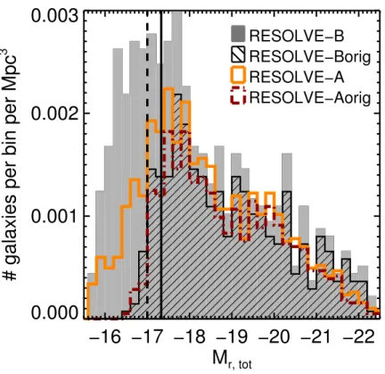
Figure 2.2: Absoluter-band magnitude distribution of RESOLVE-B and RESOLVE-A subvolumes. The black hash filled histogram and red dot-dashed outlined histograms show the original absolute r-band magnitude distributions for RESOLVE-B and RESOLVE-A respectively. Both distributions fall off rapidly below Mr,tot < −17.33. The grey shaded histogram and the orange solid outlined

histogram show the full absoluter-band magnitude distributions for B and RESOLVE-A after redshift completion efforts described in§2.2. The RESOLVE-A region is still complete only to Mr,tot = −17.33, however we are able to move the RESOLVE-B completeness limit down to

−17.0.

2.2.1: RESOLVE-A

The RESOLVE-A data set shown in Figure 2.1 occupies a volume of∼38,400 Mpc3 _{defined by:}

131.25◦ <RA <236.25◦, 0◦ < Dec < 5◦, and 4500 km s−1 <cz<7000 km s−1. The data set’s r-band absolute magnitude distribution is shown in the orange solid line histogram in Figure 2.2.

RESOLVE-A is complete down to Mr,tot < −17.33 using the reprocessed photometry described

in §2.3.1. A magnitude of Mr,tot ∼ −17.33 roughly corresponds to Mbary ∼ 109.1 M (K13). To

determine the baryonic mass completeness limit, we consider the scatter in baryonic mass-to-light ratio, which can be at least as high as 3 resulting in a baryonic mass limit of 109.3 _M_{. The}

(37)

∼12% were added from redshift surveys besides the SDSS main redshift survey. The data set resulting from the SDSS main redshift survey alone (RESOLVE-Aorig) is shown as the red dot-dashed line histogram in Figure 2.2. The RESOLVE-A region is 78% complete in HI when counting successful, unconfused HI detections and strong upper limits resulting in 1.4MHI <0.05Mstar. We

use the RESOLVE-A data set to determine our PGF calibrations, accounting for missing HI data with an iterative Monte Carlo technique akin to survival analysis (see§2.4 and §2.6).

2.2.2: RESOLVE-B

The RESOLVE-B data set is located in the SDSS Stripe 82 equatorial region, and it occupies a smaller volume of ∼13,700 Mpc3 _{defined by: 22h} _< _RA _< _3h, _−1.25◦ _< _Dec _< _1.25◦_{, and} 4500 km s−1 <cz<7000 km s−1. In Figure 2.2 the absolute r-band magnitude distribution is shown for RESOLVE-B galaxies coming from the SDSS main redshift survey as the black hashed histogram (RESOLVE-Borig), as well as for the full RESOLVE-B data set (grey filled histogram), which includes redshifts from the sources mentioned in §2.2 and extra SDSS redshift observations over the Stripe 82 footprint. The data set is complete in r-band absolute magnitude down to Mr,tot ∼= −17.0, slightly deeper than RESOLVE-A implying completeness to Mbary ∼109.1 M.

The RESOLVE-B survey contains 487 galaxies to this limit, ∼25% of which have been added by redshift surveys besides the SDSS main redshift survey. We have recovered more galaxies in RESOLVE-B than in RESOLVE-A due to the extra spectroscopic passes done by the SDSS that are not part of the main SDSS redshift survey. The RESOLVE-B region is ∼75% complete in HI data for good HI detections and strong upper limits. We use the RESOLVE-B data set to test our new PGF calibrations and compare with other calibrations from the literature (see§2.7).

2.3 Data

(38)

2.3.1: Photometric Data

We have reprocessed photometric data for the RESOLVE survey from the UV to near IR to obtain consistent, well-determined total magnitudes, and we use two to three methods of flux extrapolation per band to characterize systematic errors on the total magnitudes of the galaxies. We have also run the same pipeline on the larger volume-limited ECO (Environmental COntext) catalog (Moffett et al. 2015), which surrounds the RESOLVE-A subvolume. We use opticalugriz data from SDSS (Aihara et al. 2011), NIRJ HK from 2MASS (Skrutskie et al. 2006) and/orY HK from UKIDSS (Hambly et al. 2008), and NUV from theGALEX mission (Morrissey et al. 2007). Our NUV data are mostly MIS depth due to prioritization of the RESOLVE-A footprint late in the GALEX mission (after the FUV detector failed), while RESOLVE-B (Stripe 82) already had deep coverage in both the NUV and FUV for other programs. The SDSS optical imaging in the RESOLVE-B footprint is extra deep due to repeated imaging with typically 20 frames per location on the sky (Annis et al. 2014). With our improved photometry and realistic error measurements, we are able to measure reliable colors and perform accurate stellar mass estimation via SED modeling. Our reprocessed photometry improves over SDSS pipeline photometry in several key ways. First, we use images with improved sky subtraction coming from either Blanton et al. (2011) for SDSS or our own additional sky subtraction for 2MASS and UKIDSS. Second, we use the sum of the high S/N gri images to define the elliptical apertures, allowing us to determine the PA and axial ratio of the outer disk if present. Third, we apply these same elliptical apertures to all bands which allows us to measure magnitudes for galaxies that may not have been detected by the original automated survey pipeline in certain bands, especially low surface brightness galaxies in 2MASS, UKIDSS, and GALEX. Lastly, we use two to three non-parametric methods of total magnitude extrapolation, measuring the light from each band independently (see Figure 2.3 and§2.3.1). This last point allows for color gradients within galaxies, as opposed to the model magnitudes provided by SDSS (more details in§2.3.1), and allows us to measure systematic errors on magnitudes.

(39)

Blanton et al. (2011) and the fact that we allow color gradients in magnitude estimation. The newly reprocessed photometry does not create a tight red sequence on the color-magnitude relation as seen in the DR7 photometry, however we argue that the tight red sequence may be a consequence of these two issues in §2.3.1. We also discuss an independent validation of our methods with the NFGS survey (shown in Figure 2a of K13) in §2.3.1.

In addition to the reprocessed photometry, this paper also presents new UV observations of 19 galaxies using theSwiftUltraviolet/Optical Telescope (UVOT, Roming et al. 2005, see also Gehrels et al. 2004). We use imaging from the uvm2 filter, which has a comparable central wavelength but narrower width than the GALEX NUV filter (see Poole et al. 2008). Compared to GALEX, the pointing restrictions for UVOT are much less stringent, allowing us to obtain observations during

Swift team fill-in time for RESOLVE-B galaxies that were not observed by GALEX or had only AIS depth (∼150s) coverage. Nineteen galaxies were observed for more than 1 ks, the minimum exposure for useful photometry. Images were processed following Hoversten et al. (2011). Each galaxy was manually inspected to make sure that the surface brightness in the uvm2 band was low enough that the resulting photometry errors due to coincidence loss were below 1% (see Poole et al. 2008; Breeveld et al. 2010; Hoversten et al. 2011). We apply similar photometric processing to the

Swiftdata as to the archival data including matched elliptical apertures and multiple extrapolation techniques.

Custom Processed Data

(40)

where there is overlap between images. No additional background subtraction is done, as we are using SDSS DR8 images with the optimized sky background subtraction of Blanton et al. (2011). For 2MASS J HK and UKIDSS Y J HK, we perform additional background subtraction by fitting and subtracting a 3rd order polynomial to a region of the galaxy frame where the galaxy and other objects are masked out. Coaddition is similar to the single frame SDSS process, using SWARP to stitch together 2MASS and UKIDSS frames with a simple average to combine pixels in overlapping areas of the sky. Based on visual inspection of the UKIDSS data, we do not use theJ band due to background subtraction and other issues that affect∼75% of the data. We have also examined the Y HK images for each galaxy by eye to flag any cases with bad data. TheGALEX NUV images do not require additional background subtraction, and these images are simply coadded using SWARP and weighted by exposure time. For the Swift uvm2 images we use Source Extractor to identify and mask objects within the frame, then subtract off the median level of the non-masked areas as the sky-background.

A significant number of galaxies (∼16%) in RESOLVE have half-light diameters smaller than three times the typical r-band psf FWHM of ∼1.4”, warranting psf-matching across the optical bands and UKIDSS IR bands. For each galaxy, we use the SDSS provided psField frame to reconstruct the psf for each band at the galaxy position on the frame. First we identify the band with the worst psf seeing (typically u or g). Next we find the Gaussian σ value with which to convolve the psf of each given band to eliminate the difference between the psf of the worst band and that given band. This Gaussian σ value is then used to create a Gaussian kernel that is convolved with the galaxy cropped image. Since we have changed the pixel scale of the frames of larger galaxies, we make sure to convert the σ value into the correct pixel scale for that galaxy. For UKIDSS IR data a similar procedure is run, except that the psf for each frame is constructed from stars identified by Source Extractor. If the value of the converted σ value is less than one pixel, we do not perform the convolution. We do not psf-match the NUV, uvm2, or 2MASSJ HK bands because their typical psfs are much larger than the SDSS (∼5.5” for NUV, ∼2.5” for uvm2, and ∼2” for 2MASS). Thus aperture matched magnitude measurements for the UV and 2MASS IR will not be correct, especially for small galaxies.

(41)

under/over masking. In §2.3.1 we discuss the application of this photometric reprocessing pipeline for the ECO (Environmental COntext) catalog (Moffett et al. 2015), for which we do not check each mask by eye. Instead we use a first iteration of the pipeline to check for discrepant total and aperture magnitudes as well as cases with no valid magnitudes at the end. For the most egregious outliers, we check the masks and edit by hand where necessary.

To determine the parameters of the elliptical fit (namely the PA and ellipticity), we use an iterative procedure involving two programs. First, Source Extractor is run on each galaxy’s cropped r-band frame to find an initial guess for the center, PA, and ellipticity, and 90% light radius. Second,

we run the IRAF task ellipse on the gri coadded image using the Source Extractor quantities as inputs and allowing the PA and ellipticity, but not the center, to vary. The gri images have the highest signal-to-noise data, and by coadding these three bands, we provide the best image to feed toellipsefor determining the PA and ellipticity in the outer parts of the galaxy. The final PA and ellipticity are chosen using a median of the fits from the outer disk of the galaxy, where “outer disk” is defined between one and two times the 90%r-band light radius determined by Source Extractor. Using the final PA, ellipticity and galaxy center, we then perform a fixed ellipse fit on the gri summed image to determine the set of annuli over which to measure the galaxy surface brightness profiles for each band separately.

These same annuli are then automatically applied to theGALEX, SDSS, 2MASS, and UKIDSS data. To match the NUV andY J HK images to the SDSS images, we resample them to the pixel scale of the SDSS image. Imposing the same annuli over all bands allows us to measure the galaxy light out to its furthest extent (based ongri). For the IR bands, we are able to measure magnitudes for twice as many galaxies as the 2MASS catalog detects and for∼1.15 times as many galaxies as the UKIDSS catalog (based on public DR8plus).

(42)

one that contains two similarly sized elliptical galaxies, all three of which are so close as to make it impossible to disentangle the light from each galaxy. We find 13 systems that benefit from attempting to remove the light from a galaxy.

Embedded Galaxies: There are five systems that are heavily embedded inside a much larger galaxy: rs0675, rs0749, rs1233, rs1227, and rs0072 (inside rs0673, rs0750, rs1232, rs1226, and rs0072 respectively). Another three systems are on the outskirts of a larger galaxy: rs0639, rs1089, and rf0090 (just outside of rs0642, rs1090, and rf0094 respectively). To obtain better photometry for these eight embedded galaxies, we first mask the small embedded galaxy and run ellipse on the larger galaxy. We then subtract off the model flux from the larger galaxy that is output from

ellipse. We use the resulting image that has the large galaxy subtracted out to run through the procedures described in this section, ensuring that any residuals from the model are masked out.

Close Pairs: There are five close pair systems for which subtracting off the light of one or both of the members improves the magnitude estimates. These systems are rs0267/rs0268, rs0397/rs0398, rs0851/rs0852, rf0015/rf0016, and rf0309/rf0310. To subtract off the light of each member we use the following steps:

• First, we identify the galaxy with the simpler light profile, which we call galaxy-A. For each pair galaxy-A is rs0268, rs0397, rs0851, rf0016, and rf0310.

• Second, we start with the image for the other galaxy, which we call galaxy-B. We mask galaxy-B and run ellipse to fit the light profile of galaxy-A.

• Third, we subtract off the galaxy-A model flux as provided by ellipse from the galaxy-B image. The resulting image is used in the standard pipeline for galaxy-B (rs0267, rs0398, rs0852, rf0015, rf0309).

•In most cases, we do not then subtract off the galaxy-B image for galaxy-A. We choose not to for a variety of reasons. For rs0267/rs0268, galaxy-B (rs0267) does not have a regular light profile making it difficult to subtract off. For rs0397/rs0398 and rf0309/rf0310 galaxy-B (rs0398, rf0310) is edge-on and easy to mask. For rs0851/rs0852, galaxy-B (rs0852) is much smaller and easier to mask out.

(43)

galaxy-B image. The resulting image of galaxy-A (which is no longer in the center) is run through the pipeline with newly generated masks.

We perform these procedures for all optical bands and UKIDSS images. For 2MASS and

GALEX, we check first whether the subtraction is needed because the galaxy light may not extend far enough in these bands.

Magnitude Extrapolation

To extrapolate total magnitudes from the fixed ellipse fits for the optical bands, we use three methods: an exponential (Sersic index n = 1) fit to the outer disk, a non-parametric Curve of Growth extrapolation, and an Outer Disk Color Correction based on ther-band. Figure 2.3 shows schematics of all three methods in theg band for a RESOLVE-B galaxy.

Outer Disk Fit: To compute the outer disk flux, we first define a fitting region where the annular flux is 1 to 5 times the σ of the sky noise. If the galaxy frame has been masked heavily (due to nearby stars or galaxies), we use a region 3 to 8 times the σ of the sky noise, and in extreme cases where a bright star or galaxy is on top of the galaxy, we use a region defined by 20-50 times theσ of the sky noise. Then we fit an exponential disk function to the fitting region of the galaxy surface brightness profile (between orange and red lines in left panel of Figure 2.3) and sum the extrapolated flux from the inner edge of the last ellipse in the fitting region (red line) to an extremely large radius “R∞” or 1000” past the inner edge of the last ellipse in the fitting region (red line). To compute the inner disk flux, we sum the raw, unmodeled flux interior to the inner edge of the last ellipse in the fitting region (red ellipse in left panels of Figure 2.3). If pixels are masked in the raw data, we replace those values with the model output fromellipse. The exponential total magnitude equals the sum of the measured inner flux and the extrapolated outer disk flux. The typical dividing radius is near the 90% light radius in the r band.

(44)

changes in the total enclosed magnitude as a function or radius are small (between the light and dark green lines in the central panel of Figure 2.3). The y-intercept of the fitted line, where dm/dr = 0, is the total Curve of Growth magnitude.

0 20 40 60 80

radius (arcsec) 22 20 18 16 fit region Curve of Growth

−0.04 −0.03 −0.02 −0.01 0.00 0.01 dm/dr 17.5 17.6 17.7 17.8 17.9

g = 17.53

enclosed galaxy magnitude within radius

0 5 10 15 20

radius (arcsec) 28 26 24 22 20 µg fit region Outer Disk Fit

−30 −20 −10 0 10 20 30

∆RA (arcsec)

−30 −20 −10 0 10 20 30 ∆ Dec (arcsec)

g = 17.55

sum flux inside

use extrapolated flux outside

−30 −20 −10 0 10 20 30

∆RA (arcsec)

−30 −20 −10 0 10 20 30 ∆ Dec (arcsec) A_out Color Correction

0 5 10 15 20 25 30

radius (arcsec) 0.2 0.4 0.6 0.8 1.0 g−r

g = 17.55 determine fixed color here apply fixed color here

R70,r R90,r

Figure 2.3: Illustration of the three methods described in §2.3.1 to extrapolate the total g-band magnitude for RESOLVE-B galaxy rf0218. In this case, all three estimates agree closely (17.55, 17.53, 17.55), yielding a small systematic error (0.021). Left column: To demonstrate the Outer Disk Fit method, we show in the top left panel annular g-band surface brightness vs. radius with the fitting region marked by the orange (inner) and red (outer) lines. The blue line shows the exponential disk fit to the data points. The bottom left panel illustrates how we compute the total magnitude as the sum of the raw galaxy flux inside the radius marked by the red line (same as radius in top panel marked by red line) and the extrapolated flux outside that radius. Middle column: To demonstrate the Curve of Growth method, we show in the top middle panel enclosed galaxy magnitude vs. radius with the fitting region marked by light green (inner) and dark green (outer) lines. The lower middle panel shows the enclosed galaxy magnitude vs. the derivative of enclosed magnitude with respect to radius for the points within the fitting region defined above. The blue line shows the fit and the y-intercept at dm/dr = 0 is the total galaxy magnitude. Right column: To demonstrate the Outer Disk Color Correction method, we show in the top right panel the annulus Aout defined by the r-band 70% and 90% light radii (light and dark blue lines respectively). Using

the flux ratio in Aout, we fix the color of the galaxy to determine the g-band flux beyond R90,r,

(45)

Outer Disk Color Correction: This method scales the outer disk r-band flux to determine the outer disk flux of an object in another band. First, we use either the Curve of Growth or the Outer Disk Fit r-band magnitude to determine the radii containing 70% and 90% of the r-band light in the running total flux profile (light and dark blue ellipses show these respective radii in right most panel of Figure 2.3). If the galaxy frame is heavily masked (more than 5% of the image pixels), we prefer the r-band exponential magnitude, otherwise the r-band Curve-of-Growth magnitude is used. We next measure the galaxy flux within the R70,r to R90,r annulus (Aout). If the S/N of

the flux in this annulus is not greater than 10, we decrease the inner radius of A_out by increments of 5% down to 50% of the r-band light, stopping when we achieve S/N > 10. If the S/N is still less than 10 betweenR50,r and R90,r, we do not compute the galaxy magnitude with this method.

Otherwise, we calculate the flux ratio between a given band x and the r band within the annulus Aout, and we assume that this ratio continues out to infinity. From the r-band flux fromR90,r to

R∞, and the flux ratio within Aout, we estimate the flux in band x from R90,r to R∞, then add

this flux to the raw enclosed flux insideR90,r to get the final magnitude.

(46)

Errors for all bands are computed using not only the formal statistical error on the magnitude, but also the systematic error based on the difference in flux measured from the three methods. We apply a built in floor for the systematic error based on the overall distribution of systematic errors for the galaxy data set, such that none are lower than the original 25 percentile.

In addition we compute half light and 90% light radii in the r band (R50,r and R90,r), as well

as the r-band surface brightness within these radii (µr,50 and µr,90). We also measure aperture

magnitudes for all available bands within the r-band half light and 90% light radii, although the lack of psf correction for the 2MASS J HK and NUV and uvm2 bands compromises associated aperture matched colors. We also compute the g −r color gradient (hereafter ∆_g−r), which is

defined as the g−r color within the annulus between the half light and 75% r-band light radii minus the g−r color within the r-band half light radius. More positive colors indicate galaxies with bluer centers.

Throughout this work we use Milky Way foreground extinction corrections determined from the dust maps of Schlegel et al. (1998) with the extinction curves of O’Donnell (1994) for the optical and IR data, and of Cardelli et al. (1989) for the NUV and uvm2 data. For the NUV and uvm2 data we use the extinction correction calculated at 2271 ˚A and 2221 ˚A, the effective wavelengths of the NUV and uvm2 filter respectively. We note that using the more recently computed extinction coefficients from Schlafly & Finkbeiner (2011), which use the extinction curve from Fitzpatrick (1999), yields colors that are ∼0.015 mag bluer in u−r (∼0.04 bluer in NUV−r) and do not change the stellar mass estimates from§2.3.2.

Table 2.1 provides descriptions of the columns that are provided in a machine readable table with the photometry for the RESOLVE survey. All galaxies processed are provided, including those in the buffer and fainter than the nominal RESOLVE limits.

Table 2.1: RESOLVE Custom Photometry Catalog Description

Column Description

1 RESOLVE ID

2 Right Ascension

3 Declination

(47)

Table 2.1 – continued from previous page

4 cz

5 group cz

6 absolute SDSS r-band magnitude 7 apparent SDSS u-band magnitude 8 apparent SDSS u-band magnitude error 9 apparent SDSS g-band magnitude 10 apparent SDSSg-band magnitude error 11 apparent SDSS r-band magnitude 12 apparent SDSS r-band magnitude error 13 apparent SDSS i-band magnitude 14 apparent SDSS i-band magnitude error 15 apparent SDSS z-band magnitude 16 apparent SDSS z-band magnitude error 17 apparent GALEX NUV-band magnitude 18 apparent GALEX NUV-band magnitude error 19 apparentSwift uvm2-band magnitude 20 apparentSwift uvm2-band magnitude error 21 apparent 2MASSJ-band magnitude 22 apparent 2MASSJ-band magnitude error 23 apparent 2MASS H-band magnitude 24 apparent 2MASS H-band magnitude error 25 apparent 2MASS K-band magnitude 26 apparent 2MASS K-band magnitude error 27 apparent UKIDSS Y-band magnitude 28 apparent UKIDSS Y-band magnitude error 29 apparent UKIDSS H-band magnitude

(48)

30 apparent UKIDSS H-band magnitude error 31 apparent UKIDSS K-band magnitude 32 apparent UKIDSS K-band magnitude error 33 b/aaxial ratio of outer disk

34 R50,r half-light radius inr band

35 R90,r 90% light radius in r band

36 ∆g−r g−r color gradient

37 (u−r)m modeledu−r color 38 (u−i)m modeledu−icolor 39 (u−J)m modeledu−J color 40 (u−K)m _modeled_u₋_K _color

41 (g−r)m modeledg−r color 42 (g−i)m modeledg−icolor 43 (g−J)m modeledg−J color 44 (g−K)m modeledg−K color

45 stellar mass

46 foreground extinction in u band 47 foreground extinction ing band 48 foreground extinction inr band 49 foreground extinction in iband 50 foreground extinction inz band 51 foreground extinction in NUV band 52 foreground extinction in uvm2 band 53 foreground extinction inY band 54 foreground extinction inJ band 55 foreground extinction inH band

(49)

56 foreground extinction inK band

All magnitudes are newly measured from the raw images. Apparent magnitudes are provided without foreground extinction corrections. Foreground extinction corrections used in this work

are provided. Modeled colors designated by a superscript m are products of the SED fitting routine from K13, described in §2.3.2 and have foreground extinction corrections and

k-corrections implicitly included. The data table is provided at http://resolve.astro.unc.edu/data/resolve phot dr1.txt

Comparison with Catalog Photometry

We compare our newly reprocessed magnitudes, radii, and colors to the Petrosian and model photometry provided in the SDSS DR7 catalog in Figure 2.4. SDSS catalog Petrosian magnitudes are measured within a circular aperture of twice the Petrosian radius, defined as the radius Rp

where the ratio of the local surface brightness at Rp to the surface brightness withinRp is equal

to 0.2 (Blanton et al. 2001). The SDSS pipeline uses the Petrosian radius defined by the r band to compute Petrosian magnitudes for all other bands, thus yielding aperture-matched magnitudes and colors. The Petrosian system should pick up nearly total fluxes for disk (Sersicn= 1) galaxies, but is known to underestimate magnitudes for higher Sersicngalaxies by∼0.2 mag (Graham et al. 2005). The SDSS pipeline also computes model magnitudes by fitting exponential (n= 1) and de Vaucouleurs (n= 4) models to the galaxy light profile, choosing the model of greater likelihood in the r band, and extrapolating the profile to infinity. To measure model magnitudes for the ugiz bands, the SDSS pipeline scales the amplitude of ther-band profile up or down to best match the profile in that band (Stoughton et al. 2002). Neither magnitude system is ideal as the Petrosian magnitudes do not measure the total galaxy light, while the model magnitudes are most sensitive to the inner profile of the galaxy and do not allow for color gradients within galaxies.

In Figure 2.4a we compare our newly reprocessedr-band magnitudes with DR7 Petrosian catalog magnitudes as a function of galaxy half light radiusR50,r. The reprocessedr-band magnitudes are