CONFIDENCE REGION AND INTERVALS FOR SPARSE PENALIZED REGRESSION USING VARIATIONAL INEQUALITY TECHNIQUES
Liang Yin
A dissertation submitted to the faculty of the University of North Carolina at Chapel Hill in partial fulfillment of the requirements for the degree of Doctor of Philosophy in the
Department of Statistics and Operations Research.
Chapel Hill 2015
Approved by:
Shu Lu
Yufeng Liu
Amarjit Budhiraja
Scott Provan
c O 2015 Liang Yin
ABSTRACT
LIANG YIN: CONFIDENCE REGION AND INTERVALS FOR SPARSE PENALIZED REGRESSION USING VARIATIONAL INEQUALITY
TECHNIQUES.
(Under the direction of Shu Lu and Yufeng Liu.)
With the abundance of large data, sparse penalized regression techniques are commonly
used in data analysis due to the advantage of simultaneous variable selection and prediction.
By introducing biases on the estimators, sparse penalized regression methods can often select a
simpler model than unpenalized regression. A number of convex as well as non-convex penalties
have been proposed in the literature to achieve sparsity. Despite intense work in this area,
it remains unclear on how to perform valid inference for sparse penalized regression with a
general penalty. In this work, by making use of state-of-the-art optimization tools in variational
inequality theory, we propose a unified framework to construct confidence intervals for sparse
penalized regression with a wide range of penalties, including the well-known least absolute
shrinkage and selection operator (LASSO) penalty and the minimax concave penalty (MCP).
We study the inference for two types of parameters: the parameters under the population version
of the penalized regression and the parameters in the underlying linear model. Theoretical
convergence properties of the proposed methods are obtained. Simulated and real data examples
ACKNOWLEDGMENTS
Over the past five years I have received support and encouragement from a great number of
individuals. First and foremost I want to thank my two advisors Shu Lu and Yufeng Liu. They
provided unreserved support during my PhD and generously paved the way for my development
as a research scientist. I appreciate all they contributions of time, ideas, and funding to make
my Ph.D. experience productive and stimulating. The joy and enthusiasm they have for their
research were contagious and motivational for me, even during tough times in the Ph.D. pursuit.
The members of the Dr Liu’s group have contributed immensely to my personal time. The
group has been a source of friendships as well as good advice and collaboration. I would like
to acknowledge past and present group members Wonyul Lee, Qiang Sun, Chong Zhang, Guan
Yu, Patrick Kimes, Yuying Xie and Junlong Zhao. We had valuable discussions of research, life
and professional career.
I am also greatly indebted to the many people who in some way contributed to the progress
of the work contained herein. I would like to thank my dissertation committee members:
Kai Zhang, Amarjit Budhiraja and Scott Provan for their time, interest, helpful comments and
insightful questions. I especially appreciate the help and comments provided by Michael Lamm.
We had lots of great discussions for variational inequality techniques and shared our research
work and experience.
My time at UNC was made enjoyable in large part due to the many friends that became a
part of my life. I am grateful for time spent with roommates and friends, Tao Wang, Xinchun
Shen, Xuzhe Shen, Minghui Liu, Dong Wang, Jie Xiong, Zhe Wang, Haojin Zhai, Zhankun
Sun, Haifeng Lin, Nelson Lee, Di Miao, and for many other people and memories.
Lastly, I would like to thank my parents who raised me with a love of science and supported
TABLE OF CONTENTS
LIST OF TABLES . . . viii
LIST OF FIGURES . . . ix
1 INTRODUCTION . . . 1
1.1 Sparse penalized regression and inference for statistical modeling . . . 1
1.2 A population penalized approach for inference after penalized regression . . . 3
1.3 New contributions and key techniques . . . 5
1.4 Some preliminaries and notations on variational inequalities . . . 8
1.5 Outline of the dissertation . . . 12
2 INFERENCE FOR THE LASSO . . . 14
2.1 Introduction . . . 14
2.2 Problem transformations . . . 15
2.2.1 Conversion to a standard quadratic program . . . 15
2.2.2 The variational inequality and normal map formulation . . . 18
2.2.3 Transformations of the SAA problem . . . 21
2.3 Confidence intervals for the population LASSO parameters with fixedλ . . . 24
2.3.1 The convergence and distributions of SAA solutions . . . 24
2.3.2 Estimation of the B-derivativedΠS(z0) and the normal map LK . . . 29
2.3.3 Confidence intervals for the normal map solutions . . . 37
2.3.4 Confidence intervals for LASSO parameters . . . 38
2.4 Confidence intervals for the population LASSO parameters with varying λ . . . . 39
2.4.1 Properties ofzN and ΦN(zN) . . . 39
2.4.4 Algorithms of LASSO confidence intervals along the path . . . 53
2.5 Confidence intervals for the true parameters in the underlying linear model . . . 57
2.6 Numerical examples . . . 68
2.6.1 Example 2.6.1: Asymptotic distribution of LASSO parameters . . . 68
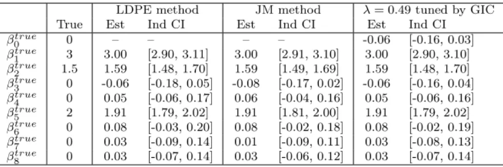
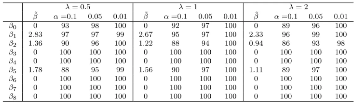
2.6.2 Example 2.6.2: Low dimensional simulation . . . 71
2.6.3 Example 2.6.3: High dimensional simulation . . . 74
2.6.4 Example 2.6.4: Coverage test for confidence bands . . . 76
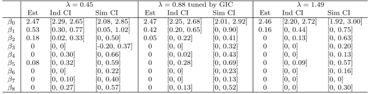
2.6.5 Example 2.6.5: Prostate cancer data . . . 78
2.7 Summary . . . 81
3 INFERENCE FOR GENERAL PENALIZED REGRESSIONS . . . 83
3.1 Introduction . . . 83
3.2 Problem transformations . . . 84
3.2.1 Transformations of the population penalized regression . . . 84
3.2.2 Transformations of the SAA problem . . . 92
3.3 Confidence intervals for population penalized parameters . . . 94
3.3.1 Convergence and distribution of SAA solutions . . . 95
3.3.2 Estimators of Σ0 and LK . . . 96
3.3.3 Confidence intervals for penalized parameters . . . 100
3.4 Confidence intervals for the true parameters in the underlying linear model . . . 101
3.5 Numerical examples . . . 106
3.5.1 Example 3.5.1: Low dimensional simulation . . . 107
3.5.2 Example 3.5.2: High dimensional simulation . . . 109
3.5.3 Example 3.5.3: Prostate cancer data . . . 111
3.6 Summary . . . 112
4 DISCUSSION . . . 114
4.1 Hypothesis testing for sparse penalized regression . . . 114
LIST OF TABLES
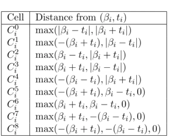
2.1 Cells in the normal manifold ofSi and the associated critical cones . . . 30
2.2 Matrix representations of ψk fork= 0,· · · ,8 . . . 31
2.3 Distances between (βi, ti) and cells in the normal manifold ofSi . . . 32
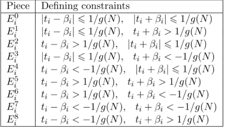
2.4 Ei0,· · ·, Ei8 in the plane (βi, ti) . . . 40
2.5 90% CIs for ( ˜β0,β) in Example 2.6.2. . . 72˜
2.6 90% individual CIs for ( ˜βtrue 0 ,β˜true) in Example 2.6.2. . . 72
2.7 Coverage of the individual CIs for ( ˜β0,β) in Example 2.6.2. . . 73˜
2.8 Coverage of the individual CIs for ( ˜βtrue0 ,β˜true) in Example 2.6.2. . . 73
2.9 Coverage and length of 95% individual CIs for ( ˜β0,β) in Example 2.6.3. . . 75˜
2.10 Coverage and length of 95% individual CIs for ( ˜β0true,β˜true) in Example 2.6.3. . . 75
2.11 95% CIs for ( ˜β0,β) in Example 2.6.5. . . 78˜
2.12 95% individual CIs for ( ˜β0true,β˜true) in Example 2.6.5. . . 79
3.1 Estimates and 95% CIs for ( ˜β0,β) and ( ˜˜ β0true,β˜true) in Example 3.5.1. . . 109
3.2 Coverage and length of 95% individual CIs for ( ˜β0,β) in Example 3.5.1. . . 110˜
3.3 Coverage and length of 95% individual CIs for ( ˜β0true,β˜true) in Example 3.5.1. . . 110
3.4 Coverage and length of 95% individual CIs for ( ˜β0,β) in Example 3.5.2. . . 111˜
3.5 Coverage and length of 95% individual CIs for ( ˜β0true,β˜true) in Example 3.5.2. . . 111
LIST OF FIGURES
1.1 The normal and tangent cones of the polyhedron S. . . . 9
2.1 The normal manifold of Si. . . 30
2.2 Ei0,· · ·, Ei8 in the plane (βi, ti) . . . 40
2.3 Distribution of SAA solutions in Example 2.6.1 . . . 71
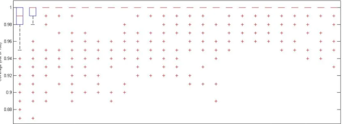
2.4 Boxplot of coverage rates of 95% individual CIs for z0 in Example 2.6.4 . . . 77
2.5 Boxplot of coverage rates of 95% individual CIs for ( ˜β0,β) in Example 2.6.4 . . . 77˜
2.6 95% Confidence bands for ( ˜β0,β) in Example 2.6.5. . . 80˜
CHAPTER 1: INTRODUCTION
1.1 Sparse penalized regression and inference for statistical modeling
In recent years, significant developments have been made in high dimensional data analysis
driven by the great needs in different scientific disciplines. Theory and methodology that
are developed in modern research are generally guided by the following two aspects: (1) It
is desirable for investigators to understand the mechanism in the data with a parsimonious
model, to be found through data-driven model selection; and (2) Investigators often need to
make statistical inference from the model they select. These two aspects, variable selection and
inference, are two central issues in statistical modeling, which are particularly important when
a large set of candidate explanatory variables is available for the model.
Regarding data-driven model selection procedures, traditional statistical methods such as
ordinary least squares regression often give poor prediction accuracy and are weak in model
interpretation for high dimensional problems. With the advantage of simultaneous variable
selection and prediction, sparse penalized regression has been widely used. By introducing
bi-ases on the resulting estimators through sparse penalization, these methods can often produce
estimators with much smaller variances and consequently lower mean square errors than
un-penalized estimators. Furthermore, because of the built-in sparsity on the estimators, model
selection and parameter estimation can be achieved in a single step. There is a large literature
in this area including the L1 regularized technique LASSO [11; 49], as well as many other
ex-tensions with different settings or penalties, see [18; 15; 60; 28; 59; 9; 51; 29; 33; 46; 55; 47],
and many more. Lots of these extensions aim to obtain estimators with better properties such
as lower bias [15; 55] and with structure [5; 53; 57; 58]. For computation, fast implementations
have been proposed to handle data of very high dimensions. For example, the LARS algorithm
by [13], the Coordinate-Descent algorithm by [52], and the Glmnet algorithm by [17] are three
After the data-driven selection, one common practice is to carry out conventional inference
on the selected model. Despite its prevalence, this practice is problematic because it ignores
the fact that the inference is conditional on the model selection that is itself stochastic. The
stochastic nature of the selection process affects and distorts sampling distributions of the
post-selection parameter estimates, leading to invalid post-selection inference. The problems of
post-selection inference have long been recognized and have been discussed recently by [2; 6;
25; 26; 27].
In recent years, many methods have been developed to achieve valid inference after LASSO.
We refer to [8] for a comprehensive review on these developments. We categorize these methods
into the following three types of approaches:
The simultaneous inference approach. This approach is guided by a general heuristic to consider all possible outcomes of the selected model and protect the valid inference for
the worst scenario. Papers along this line include [3; 10; 36].
The bias-correction approach. This approach considers adjusting for the bias that is introduced by the regularization step to achieve valid inference. Papers along this line
include [7; 21; 56; 50].
The conditional sampling distribution approach. This approach aims at understanding the asymptotic or exact distributions of some pivots conditional on the selected model
and developing inference methods based on these distributions. Papers along this line
include [24; 30].
Although so far there have been many methods can do inference after LASSO, the inference for
other penalized regression is still untouched. Fan and Li [15] pointed out three properties for
a good regularization penalty. The first one is sparsity. In order to reduce model complexity,
regularized regression estimators should automatically set small coefficients to zero. Penalties
with singularity at zero, such as LASSO, fulfill this requirement. The second one is the nearly
unbiasedness. Although we must introduce biases for sparsity, we want the resulting estimators
proposed to reduce the model bias, such as SCAD [15] and MCP [55] penalties. These penalties
do not over penalize coefficients when the true coefficients are large. The last property is that
the resulting estimators should be continuous with respect to the tuning parameter to improve
stability in model prediction. A penalty function must be singular at the origin if it satisfies the
first and third conditions. Therefore, the general penalized regressions with sparse penalties
which may have these three properties deserve their own inference method.
1.2 A population penalized approach for inference after penalized regression
In this dissertation, we take a different view of the penalized regression and utilize the
state-of-the-art stochastic variational inequality theory in optimization to construct confidence
regions and confidence intervals. Consider the standard linear regression setting in which the
penalized regression solves
min
β0,β
1
Ny−β01N −Xβ
2 2+
p
∑
j=1
Pλj(|βj|), (1.1)
where y, y1 y2 .. . yN
, X,
x11 x12 · · · x1p
x21 x22 · · · x2p
..
. ... . .. ...
xN1 xN2 · · · xN p
= x1 x2 .. . xN
, 1N =
1 1 .. . 1
∈RN,
and (x1, y1),· · · ,(xN, yN) are independent samples. For each i= 1,· · · , N and j = 1,· · · , p,
xij ∈R,yi ∈Randxi ∈Rp. We use bold font to present data vectors and matrices. β0 ∈Rand
β = (β1,· · ·, βp)T ∈Rp are the regression parameters. Pλj(| · |) is a general penalty forβj with
the regularization parameter λj >0. This general penalty covers the L1 penalty, the adaptive
LASSO penalty [59], or any other nonconvex penalty such as SCAD or MCP. Our interest is
penalized regression by solving
min
β0,β
E[Y −β0− p
∑
i=1
βiXi
]2
+
p
∑
j=1
Pλj(|βj|), (1.2)
where X = (X1,· · ·, Xp)T ∈ Rp is an explanatory random vector, and Y ∈ R is a response
random variable. We refer to (1.1) as the sample average approximation (SAA) problem of the
population penalized problem (1.2). Denote the solution to the SAA problem (1.1) as ( ˆβ0,β),ˆ
which we refer to as penalized estimators. We will make use of the penalized estimators ( ˆβ0,β)ˆ
to derive confidence intervals and regions for the population penalized parameters ( ˜β0,β) as˜
the solution of (1.2).
The population penalized approach is closely related to the traditional least squares
ap-proach. When penalty terms Pλj(|βj|) all take the value of 0, the problem (1.2) becomes the
following population least squares problem:
min
β0,β
E[Y −β0− p
∑
j=1
βjXj]2, (1.3)
which has a unique minimizer (E[XXT])−1E[XY] when E[XXT] is invertible. If additionally X and Y are related by the following linear model
Y =β0true+XTβtrue+ε (1.4)
with E[ε|X] = 0, then this solution to the population least squares problem (1.3) is
ex-actly (β0true, βtrue). When penalty terms Pλj(|βj|) > 0, the solution to (1.2) is not exactly
(βtrue
0 , βtrue), but is related to (β0true, βtrue) in a different way. We will also develop a method
which utilizes that relation to construct confidence intervals for the true parameters above in
the linear model (1.4).
Why could the minimizer from a population penalized regression be a reasonable target for
scientific research? While it is apparent that a selection procedure such as LASSO is necessary
it is well-known that including nearly collinear redundant variables in a regression model can
“adjust away” some of the causal variables of interest (see discussions in Section 2 in [3]).
Moreover, using the full model could be questionable in areas such as social science [1]. In
these areas, it is common that when the question of “which variables should be included in
the regression model” is asked, the scientific theory is not sufficient enough to dictate the
inclusion or exclusion of variables for the inference (even when N > p). In this case, a
data-driven model from sparse penalized regression would be helpful and more compelling. However,
under this situation, the goal of the inference is slightly changed from that of the least squares
approach: The investigator is no longer looking for the least squares coefficients that minimize
the squared error loss in the population. Instead, she wants to find the least squares estimate
subject to certain regularization on the model. Thus, this application of penalized regression
leads naturally to the consideration of the population penalized parameters as the target of
inference. On the other hand, under appropriately chosen nonconvex penalties, the difference
between the population penalized parameters and the least squares regression parameters would
be very small. Therefore in this case the inference for population penalized parameters is
approximately valid for the least squares regression parameters.
The regularization scheme mentioned above relates closely to the regularization terms
Pλj(|βj|).The major difference between the population penalized approach and the least squares
approach is the incorporation of constraint information about the model/parameters. Though
the source of such information can be from different perspectives, they can all be reflected in the
penalty terms withλj as a measure of the strength of such information. Thus, the parameters
in the population penalized approach are both scientifically and statistically meaningful: They
lead to the best approximations to the response when external information is available. This
interpretation is valid both for N < pand for N > p.
1.3 New contributions and key techniques
In the work for this dissertation, the first contribution is to make use of the penalized
(include nonconvex penalization) estimators ( ˆβ0,β) to derive confidence intervals and regionsˆ
penalized parameters is based on study of the asymptotic distribution of penalized estimators
(i.e., solutions to (1.1)), as they converge to the population penalized parameters (solution to
(1.2)). A good understanding of such asymptotics around the population penalized parameters
(as the right asymptotic target) will in turn provide important insights for the inference of
true parameters in the linear model (1.4). We also note here that inferences for the population
penalized parameters are by themselves meaningful probabilistic statements that are of practical
use.
Since penalized estimators are obtained by solving (1.1), they depend on random samples and are subject to uncertainty. Our inference results provide quantitative measures about
the level of such uncertainty, by estimating the distance between the population penalized
parameters and the computed penalized estimators. Sizes of those intervals are jointly
determined by sample variability and sensitivity of penalized estimators with respect to
random samples. Wide intervals indicate low reliability of the estimators, which can be
caused by large sample variability or high sensitivity. Thus, these inference results can
be used as quantitative assessments on the reliability and uncertainty level of penalized
estimators obtained from (1.1).
The inference results of this work can be used to assess the relative importance of pre-dictors. For nonzero penalized estimators, conclusions can be made regarding whether
the corresponding parameters are truly nonzero by checking if the corresponding intervals
contain zero or not. For zero penalized estimators, the inference results can be highly
informative as well. For example, if the confidence intervals of some penalized parameters
are singletons of zero, then we have strong evidence to conclude that the corresponding
population penalized parameters are zero.
Besides inference for the penalized parameters, the second contribution of this work is to
develop an inference method for the true parameters in the linear model (1.4) via the
penal-ized regression. Our method is based on a relationship between ˜β and βtrue as well as their
decomposition:
ˆ
β−βtrue= ˆβ| {z }−β˜
(∗)
+ ˜β| {z }−βtrue
(∗∗)
. (1.5)
In a sense, the decomposition in (1.5) is similar as the bias-variance decomposition. Through the
population penalized approach, we are able to quantify the uncertainty in (∗) (or the “variance”
part). Since the population penalized parameters ˜β is the asymptotic limit of the penalized
estimators ˆβ, the limiting distribution of (∗) characterizes the variation around ˜β. Through
a connection between ˜β and βtrue that corrects the “bias” in (∗∗), we are able to provide
valid inference for the true parameters. This method belongs to bias-correction category and is
especially useful when the biases introduced by the penalization are large. Simulation results
show that under LASSO regression our method performs competitively with existing methods
with some gains on the width of confidence intervals for inactive variables in high dimensions.
In this dissertation, we develop the theories based on the fixed dimension p, although it is
possible to extend this idea to the case of growing dimensions. The development of our method
takes the following steps. First, we transform the problems (1.1) and (1.2) into their
correspond-ingnormal map formulations, which are equations with a (2p+ 1)-dimensional variable vector
z. Next, we obtain the asymptotic distribution of solutions to the normal map formulation
of (1.1), and find reliable estimates for quantities that appear in the asymptotic distribution.
We then provide methods to compute simultaneous and individual confidence intervals for the
solution to the normal map formulation of (1.2). Finally, we convert these confidence intervals
into confidence intervals for the solution to (1.2). Note that our inference method is developed
for fixed penalties Pλj(|βj|). In practice, the tuning parameters in the penalty terms can be
chosen by various criteria or through cross validation.
At last, inspired by existing LASSO path algorithms such as [13], we are interested in the
confidence band constructed by consecutively computing confidence intervals along the LASSO
solution path with respect to tuning parameter λ. The third contribution of this work is
to point out that our confidence intervals for the population LASSO parameters along their
solution path have the “piecewise Lipschitz property” under some mild assumptions (That
Lipschitz continuous inλ), and to propose a linear approximation algorithm to track the entire
confidence band. We only calculate CIs on the two ends of aλinterval on which the boundaries
of the confidence band are Lipschitz, then we link the corresponding boundaries of these two
confidence intervals to make an approximated confidence band on this interval. There are two
key issues for this algorithm: Finding theλknots which are cut-off points for piecewise Lipschitz
property and calculating confidence interval on these knots. According to our experience, the
number of suchλknots is O(p), but unfortunately the computation for confidence intervals at
some knots is very expensive. For the computational reason, we suggest a way to modify this
tracking algorithm into a more efficient version for computing confidence intervals on a grid ofλ
values, by avoiding those computationally expensive λknots. The tracking algorithm provides
computational advantage when the confidence intervals are desired at many values of λ.
1.4 Some preliminaries and notations on variational inequalities
This section introduces some preliminary knowledge about variational inequalities, their
relation with optimization problems, the normal map formulation, and normal manifolds. The
book [14] provides a comprehensive treatment on finite dimensional variational inequalities.
The normal map formulation for variational inequalities and normal manifolds for polyhedrons
were introduced in [39; 40]. Detailed discussions on normal and tangent cones, faces, and
relative interiors are contained in [42] and [43].
We start with definitions of normal cones and tangent cones. Let S be a closed, convex set
inRn, and let x∈S. The normal cone toS atx is denoted byNS(x) and is defined as
NS(x) ={v∈Rn| ⟨v, s−x⟩ ≤0 for each s∈S}.
The tangent cone toS atx is denoted byTS(x) and is defined as
TS(x) ={w∈Rn| ∃{xk} ⊂S and {τk} ⊂Rsuch thatxk→x, τk→0, and (xk−x)/τk→w}.
sequence of points in S, and NS(x) contains all the “normal” vectors to S at x. It is easy to
see that NS(x) and TS(x) are indeed cones (a subset of Rn is a cone if a positive multiple of
any element of it still belongs to it). In fact, NS(x) and TS(x) are the polar cones of each
other, in the sense that the inner product of any element inNS(x) and any element inTS(x) is
nonpositive, see, e.g., Proposition 1.3.2 of [14].
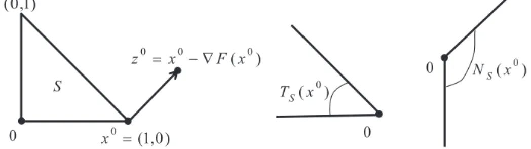
To illustrate these concepts, consider the polyhedron S in Figure 1.1, defined as S ={x∈
R2|x
1+x2 ≤1, x1 ≥0, x2≥0}. Letx0 = (1,0). For the moment, ignorez0 in the figure. The
middle graph shows the tangent cone TS(x0), which is {w ∈R2 |w1+w2 ≤ 0, w2 ≥ 0}. The
right graph shows the normal cone NS(x0) ={v∈R2|v1−v2 ≥0, v1≥0}.
) 0 , 1 (
0 =
x S
0 0
) (x0 T
S
) (x0 N
S
0 )
( 0
0 0
x F x
z = -Ñ
) 1 , 0 (
Figure 1.1: The normal and tangent cones of the polyhedronS.
Given a closed, convex set S ⊂Rn, and a function f :Rn →Rn, the variational inequality
associated with (f, S) is the problem of findingx∈S such that
0∈f(x) +NS(x). (1.6)
Here,f(x) +NS(x) is a set consisting of n-dim vectors of the form f(x) +v forv ∈NS(x). If
the set f(x) +NS(x) contains the origin ofRn, thenx is a solution of (1.6).
To see how a variational inequality is related to an optimization problem, consider the
problem of minimizing a function F :Rn → Rover a closed and convex set S. If x0 ∈ S is a local solution to this minimization problem and F is differentiable at x0, then x0 satisfies the following variational inequality:
To prove (1.7), choose a points∈S and consider the line segment connecting x0 and s. Since x0 is a local minimum of F we have ⟨∇F(x0), s−x⟩ ≥ 0. The latter inequality holds for any s ∈ S, which gives (1.7) in view of the definition of NS(x0). Conversely, if x0 satisfies (1.7)
and F is a convex function, thenx0 is a global minimizer ofF over the setS, because for each s∈S one hasF(s)−F(x0)≥ ⟨∇F(x0), s−x⟩ ≥0.
A variational inequality can be equivalently formulated as an equation using a concept
called thenormal map. To introduce this concept, let us first consider, for a fixed pointz∈Rn,
the problem of minimizing F(x) = 12∥z−x∥2 over the set S. Applying the relation between optimization and variational inequalities, and noting∇F(x) =x−z, we find that the Euclidean
projection ΠS(z) is exactly the solution of the following inclusion
z−x∈NS(x).
Now, we define the normal map induced by f and S, denoted byfS, to be a function from Rn
toRn given by
fS(z) =f(ΠS(z)) + (z−ΠS(z)) for eachz∈Rn, (1.8)
where ΠS(·) denotes the Euclidean projector onto S. One can then show for any solutionx of
(1.6) that the pointz=x−f(x) satisfies ΠS(z) =x and
fS(z) = 0. (1.9)
Conversely, for any solution z of (1.9), the point x= ΠS(z) is a solution of (1.6) and satisfies
z=x−f(x). Equation (1.9) is the normal map formulation of (1.6).
Let us revisit the example in Figure 1.1 to illustrate above concepts. Suppose F(x) =
1
2(x1−1.5) 2+1
2(x2−0.5)
2. It follows that∇F(x0) = (−0.5,−0.5), with−∇F(x0) = (0.5,0.5)∈
NS(x0). Hence, x0 satisfies (1.7). Let z0 =x0− ∇F(x0) = (1.5,0.5). Then ΠS(z0) = x0, and
z0 satisfies
which means thatz0 is a solution to (1.9) with ∇F in place off.
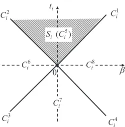
If the setS is a polyhedron inRn(a set defined by finitely many affine constraints), then the
Euclidean projector ΠS is apiecewise affine function fromRntoRn: it coincides with an affine
function on each of finitely manyn-dimensional polyhedrons whose union isRn(the dimension
of a convex set is defined to be the dimension of its affine hull, which is the smallest affine set
containing the set). Those polyhedrons, along with their faces, are called cells in the normal
manifold of S. We call a cell with dimension k a k-cell. The relative interiors of all cells in
the normal manifold form a partition of Rn (the relative interior of a convex set is its interior
relative to its affine hull). For the setS in Figure 1.1, ΠS is a piecewise affine function with 7
pieces. For example, ΠS(z) =zfor pointszbelonging toS, ΠS(z) = (0, z2) for points in the set {z∈R2 |z1≤0,0≤z2≤1}, and ΠS(z) = (0,0) for points in the set {z∈R2|z1 ≤0, z2 ≤0}.
Those sets are 2-cells in the normal manifold of S. The halfline{z∈R2 |z1 ≤0, z2 ≤0} and
the edge {z∈R2 |z1 = 0,0≤z2≤1} are 1-cells. In total, there are seven 2-cells, nine 1-cells,
and three 0-cells (vertices ofS).
Throughout this dissertation, we use ∥ · ∥ to denote the norm of an element in a normed
space; unless explicitly stated otherwise, it can be any norm, as long as the same norm is used
in all related contexts. We use N(0,Σ) to denote a Normal random vector with covariance
matrix Σ. Weak convergence of random variables Yn to Y will be denoted as Yn ⇒ Y. A
function g:Rn → Rm is said to be B-differentiable at a point x0 ∈ Rn if there is a positively
homogeneous functionG:Rn→Rm, such that
g(x0+v) =g(x0) +G(v) +o(v).
The above function G is the B-derivative of g at x0 and will be written as dg(x0). For each
h∈Rn,dg(x0)(h) is exactly the directional derivative ofgatx0 for the directionh. In general,
B-differentiability is stronger than directional differentiability, as it requires dg(x0)(·) to be a
1.5 Outline of the dissertation
In this dissertation, we will discuss how to use variational inequality techniques to compute
confidence intervals for sparse penalized regression based on the penalty term. The main outline
of this dissertation is as follows:
In Chapter 2, we consider the LASSO regression and transform LASSO problems in-to variational inequalities in-to derive confidence intervals and regions for the population
LASSO parameters. In terms of the true parameters in the underlying linear model, we
propose a method to derive confidence intervals and compare them with existing methods
in the literature. Moreover, we study the confidence bands for the population LASSO
parameters along the LASSO solution path. We point out that the entire confidence band
is neither piecewise linear nor continuous with respect to λ, if we construct confidence
band pointwisely by using techniques described in this Chapter. We also propose a linear
approximation tracking algorithm to compute confidence intervals.
In Chapter 3, we consider a general penalized regression with the penalty term satisfying the three properties suggested by [15]. We propose a unified method to construct
con-fidence intervals of the population penalized parameters for these penalized regressions,
such as LASSO and MCP regression. For the true parameters in the underlying linear
model, by correcting the bias introduced by the penalty term, we obtain asymptotic
dis-tribution of the true model estimator to construct the confidence intervals. Technically,
we propose another problem transformation approach for the penalized regression
opti-mization problem with general penalties, and extend those asymptotic results obtained
in Chapter 2.
In Chapter 4, we discuss two possible future directions. For the first direction, we point out that it is not trivial to conduct hypothesis testing and find the corresponding
p-value for the population penalized parameters and the true model parameters using the
CHAPTER 2: INFERENCE FOR THE LASSO
2.1 Introduction
In this Chapter, we discuss the inference after the LASSO regression, which is probably the
most popular method in the family of sparse penalized regression with convex penalties. We
consider the following population version of the random design LASSO problem
min
β0,β
E[Y −β0− p
∑
i=1
βiXi
]2
+λ
p
∑
i=1
|βi|, (2.1)
whereX = (X1,· · · , Xp)T ∈Rp is an explanatory random vector, Y ∈Ris a response random
variable,λ >0 is the regularization parameter, and β0 ∈Rand β = (β1,· · · , βp)∈Rp are the
regression parameters. The random design is commonly used to select a well performed model
for out-of-sample prediction of population, which is of primary concern in many applications.
The solution of (2.1) can be estimated by the solution of the corresponding SAA problem
min
β0,β
1
Ny−β01N −Xβ
2 2+λ
p
∑
i=1
|βi|, (2.2)
where y, y1 y2 .. . yN
, X,
x11 x12 · · · x1p
x21 x22 · · · x2p
..
. ... . .. ...
xN1 xN2 · · · xN p
= x1 x2 .. . xN
, 1N =
1 1 .. . 1
∈RN,
and (x1, y1),· · ·,(xN, yN) are independent samples of (X, Y). For each i = 1,· · ·, N and
population LASSO parameter ( ˜β0,β) (the solution of (2.1)) as the sample size˜ N goes to∞. In
order to indicate the reliability of this LASSO estimator, we construct confidence interval (CI)
for the population LASSO parameter. For the linear model (1.4), we also propose a method to
produce confidence intervals for the true parameters (β0true, βtrue) (which solves (1.3)).
In Section 2.2, one can see how we transform the population LASSO problem (2.1) and its
corresponding SAA problem (2.2) to their normal map formulations. The assumptions needed in
this Chapter are also listed in this section. In Section 2.3, we show the methodology of producing
confidence intervals for the population LASSO parameters at a fixed value of the regularization
parameterλ. Whenλchanges, in Section 2.4 we study the properties of the confidence bands
along the LASSO solution path, and propose sufficient algorithms to construct such bands. In
Section 2.5, we establish a connection between the population LASSO parameters ( ˜β0,β) and˜
the true parameters (β0true, βtrue). We use this connection to give an estimator of (βtrue0 , βtrue), which we denote as ( ˆβ0true,βˆtrue), and obtain the asymptotic distribution of ( ˆβtrue0 ,βˆtrue) with fixed dimension p. Numerical results are presented in Section 2.6 to illustrate the performance
of the proposed methods.
2.2 Problem transformations
In this section, we describe how to transform (2.2) and (2.1) into variational inequalities and
normal map formulations, from where we obtain the asymptotic distribution of SAA solutions.
2.2.1 Conversion to a standard quadratic program
In this subsection, we transform the population LASSO problem into a standard quadratic
programming problem. We need Assumption 2.1(a) below to guarantee the objective function
of (2.1) to be finite valued. We will use the stronger Assumption 2.1(b) in proving convergence
results.
To eliminate the nonsmooth term ∑pj=1|βj|from the objective function of (2.1), we
intro-duce a new variable t∈Rp into (2.1). The transformed problem is
min
β0,β,t
E[Y −β0− p
∑
j=1
βjXj]2+λ p
∑
j=1
tj
tj −βj ≥0, j= 1,· · · , p
tj +βj ≥0, j= 1,· · · , p.
(2.3)
We useS to denote the feasible set of (2.3):
S ={(β0, β, t)∈R×Rp×Rp |tj−βj ≥0, tj+βj ≥0, j= 1,· · · , p}. (2.4)
If we write
(β0, β, t) = (β0, β1, t1, β2, t2,· · · , βp, tp), (2.5)
then we can treat the setS as a Cartesian product:
S=R×
p
∏
i=1
Si, (2.6)
where for eachi= 1,· · · , p the setSi is a subset of R2 defined as
Si ={(βi, ti)|ti−βi ≥0, ti+βi ≥0}. (2.7)
Note that in equation (2.5) two ways of ordering elements in (β0, β, t) are used. We refer to the
ordering on the right hand side in (2.5) as “cross” ordering, and the ordering on the left hand
side as “block” ordering. Unless explicitly stated otherwise, vectors and matrices are ordered
using “block” ordering.
In the next subsection we will transform (2.3) into a variational inequality. This requires
Rp×Rp×R→R2p+1 by
F(β0, β, t, X, Y) =
−2(Y −β0−
∑p
j=1βjXj) −2(Y −β0−
∑p
j=1βjXj)X1
.. .
−2(Y −β0−
∑p
j=1βjXj)Xp
λep , (2.8)
where ep is the p-dimensional vector with all entries being 1. Clearly, F is a continuously
differentiable function, and its derivative with respect to (β0, β, t) at (β0, β, t, X, Y) is given by
d1F(β0, β, t, X, Y) =
2 2XT 0
2X 2XXT 0
0 0 0
. (2.9)
Next, define a function f0 :R×Rp×Rp →R2p+1 by
f0(β0, β, t) =E[F(β0, β, t, X, Y)]. (2.10)
Assumption 1(a) guarantees f0 to be well defined and finite valued. Moreover,f0 is an affine
function, with its Jacobian matrix being
L=E[d1F(β0, β, t, X, Y)] =
2 2E[XT] 0
2E[X] 2E[XXT] 0
0 0 0
. (2.11)
The following lemma is relatively straightforward and its proof is omitted.
Lemma 2.1. Suppose Assumption 2.1(a) holds. Then, the objective function of (2.3)is a finite valued, convex quadratic function onR2p+1, its gradient at each(β
0, β, t)∈R2p+1 isf0(β0, β, t),
and its Hessian matrix isL.
Assumption 2.2. Let ( ˜β0,β)˜ be an optimal solution of (1.2), define t˜∈Rp andq˜∈Rp by
˜
ti =|β˜i|and q˜i =E[−2(Y −β˜0− p
∑
j=1
˜
βjXj)Xi]f or each i= 1,· · · , p.
Let I be a subset of {1,· · ·, p} defined as
I=
{
i∈ {1,· · · , p} | β˜i ̸= 0 or ( ˜βi = 0 and |q˜i|=λ)
} ,
and letLI be the submatrix of Lin (2.11) that consists of intersections of columns and rows of
L with indices in {1} ∪ {i+ 1, i∈I}. Assume that LI is nonsingular.
In the above assumption, the vector ( ˜β0,β,˜ ˜t) is indeed a solution of (2.3), and Q is a
submatrix of the upperleft (p+ 1)×(p+ 1) submatrix ofL. Lemma 2.2 of the next subsection
will show that the non-singularity of Q guarantees ( ˜β0,β) to be the global unique solution of˜
(2.1).
2.2.2 The variational inequality and normal map formulation
In view of Lemma 2.1, we can rewrite (2.3) as the following variational inequality:
−f0(β0, β, t)∈NS(β0, β, t). (2.12)
If we would introduce multipliers for constraints defining S in (2.4), we could write down an
explicit expression for NS(β0, β, t) and accordingly rewrite (2.12) into the well-known
Karush-Kuhn-Tucker conditions. However, that approach would lead to more variables (the multipliers)
in the formulation and we would need additional assumptions to ensure the uniqueness of
multipliers. For this reason, we choose to deal with (2.12) directly.
Let (f0)S be the normal map induced byf0 and S, as defined in (1.8) withf0 in place of f.
The normal map formulation for (2.12) is
wherez is a variable of dimension 2p+ 1.
As noted right below Assumption 2.2, the vector ( ˜β0,β,˜ t) is a solution of (2.3). It is therefore˜
a solution of (2.12) as well. By the relation between variational inequalities and normal maps,
the point z0∈R2p+1 defined as
z0= ( ˜β0,β,˜ ˜t)−f0( ˜β0,β,˜ ˜t) (2.14)
is a solution to (2.13) and satisfies ΠS(z0) = ( ˜β0,β,˜ ˜t). LetKbe thecritical conetoSassociated
withz0, defined as
K ={w∈TS(ΠS(z0))| ⟨z0−ΠS(z0), w⟩= 0}
={w∈TS( ˜β0,β,˜ t)˜ | ⟨f0( ˜β0,β,˜ ˜t), w⟩= 0}.
(2.15)
Using the special polyhedral structure ofS, we will give an explicit expression ofKin the proof
of Lemma 2.2 below. Critical cones are commonly used in optimization to define conditions
on optimality and local uniqueness of solutions, see, e.g., [38]. We use critical cones here for
the same purposes, but also for writing down an expression of the asymptotic distribution of
SAA solutions. Let LK be the normal map induced by the linear function L as in (2.11) and
the cone K, defined as in (1.8) with L and K in place off and S respectively. In Lemma 2.2
below, we show thatLK is a global homeomorphism fromR2p+1 toR2p+1, that is, a continuous
bijective function from R2p+1 toR2p+1 whose inverse function is also continuous. The inverse function of LK will appear in an expression for the asymptotic distribution of SAA solutions.
Lemma 2.2. Suppose that Assumptions 2.1(a) and 2.2 hold. Then the normal map LK is
a global homeomorphism from R2p+1 to R2p+1, and ( ˜β0,β,˜ ˜t) is the unique optimal solution of
(2.3).
Proof of Lemma 2.2. We start by examining the structure ofK. In view of (2.6), the tangent and normal cones toS at ( ˜β0,β,˜ ˜t) can be written as
and
NS( ˜β0,β,˜ t) =˜ {0} ×NS1( ˜β1,t˜1)× · · · ×NSp( ˜βp,˜tp).
Let ˜q be as defined in Assumption 2.2, and let ˜q0 = E[−2(Y −β˜0 −
∑p
j=1β˜jXj)]. Since
f0( ˜β0,β,˜ t) = (˜˜ q0,q, λe˜ p) and −f0( ˜β0,β,˜ ˜t)∈NS( ˜β0,β,˜ ˜t), we have
˜
q0= 0 and −(˜qi, λ)∈NSi( ˜βi,t˜i) for each i= 1,· · ·, p. (2.16)
Now choose an arbitrary v∈TS( ˜β0,β,˜ ˜t), and write it as
v= (v0, v1,· · ·, vp)
withv0 ∈Rand vi ∈TSi( ˜βi,˜ti) for each i= 1,· · · , p. It is not hard to see that v belongs to K
if and only if ⟨−(˜qi, λ), vi⟩= 0 for each i= 1,· · ·, p. We can therefore writeK as
K=R×K1× · · · ×Kp
where
Ki ={vi ∈TSi( ˜βi,t˜i)| ⟨−(˜qi, λ), vi⟩= 0}for each i= 1,· · · , p.
From (2.45), for each i= 1,· · · , pwe have
Ki =
{(0,0)} if ( ˜βi = 0 and|q˜i|< λ), {(βi, ti)∈R2+|βi−ti= 0} if ( ˜βi = 0 and ˜qi=−λ), {(βi, ti)∈R2 |βi−ti = 0} if ˜βi>0,
{(βi, ti)∈R−×R+|βi+ti = 0} if ( ˜βi = 0 and ˜qi=λ), {(βi, ti)∈R2 |βi+ti = 0} if ˜βi<0.
(2.17)
N as follows:
M =
1 0
0 Ip
0 Ip
and N =
1 0
0 Ip
0 −Ip
,
where Ip is the p×p identity matrix. Construct a matrix Ξ by first adding the common first
column of M and N and then adding the i+ 1’th column of M (N) if the condition in the
second or third (fourth or fifth) row of (3.20) is satisfied. Columns of Ξ form a basis of the
affine hull ofK. It is not hard to check that ΞTLΞ =Q, whereQis defined in Assumption 2.2.
The latter assumption ensures Q to be nonsingular, so it is positive definite. It follows from
an application of [39, Theorem 4.3] that LK is a global homeomorphism. By [40, Theorem 3],
( ˜β0,β,˜ t) is a locally unique solution to (2.12). Thus, it is a locally unique solution to (2.3).˜
But the objective function of (2.3) is convex, so ( ˜β0,β,˜ ˜t) is indeed the global unique solution
of (2.3).
In the rest of this chapter, we use Σ0 to denote the covariance matrix of F( ˜β0,β,˜ ˜t, X, Y),
and let Σ10 be the upper left (p+ 1)×(p+ 1) submatrix of Σ0. Since the last p elements of
F( ˜β0,β,˜ ˜t, X, Y) are fixed atλ, we have
Σ0 =
Σ
1 0 0
0 0
. (2.18)
In addition, we make the following non-degeneracy condition
Assumption 2.3. The determinant of Σ10 defined in (2.18) is strictly positive.
2.2.3 Transformations of the SAA problem
So far we have reformulated (2.1) as a quadratic program (2.3), a variational inequality
(2.12), and an equation involving the normal map (2.13). We can reformulate the SAA problem
problem:
min
(β0,β,t)∈S
1
Ny−β01N−Xβ
2 2+λ
p
∑
j=1
tj, (2.19)
whereS is as defined in (2.4). We define theSAA function
fN(β0, β, t) =N−1 N
∑
i=1
F(β0, β, t,xi, yi),
where F is as in (2.8). By noting that fN(β0, β, t) is exactly the gradient of the objective
function of (2.19) at (β0, β, t), we can rewrite (2.19) as a variational inequality
0∈fN(β0, β, t) +NS(β0, β, t). (2.20)
The abovefN is an affine function with its Jacobian matrix given by
LN =dfN(β0, β, t) =
2 2∑Ni=1xi/N 0
2∑Ni=1(xi)T/N 2∑Ti=1(xi)T(xi)/N 0
0 0 0
. (2.21)
Finally, we let (fN)S be the normal map induced by fN and S, and write the normal map
formulation of (2.20) as
(fN)S(z) = 0. (2.22)
In Section 2.3 we will discuss the asymptotic distributions and convergence rates of solutions of
(2.20) and (2.22), and generate confidence regions and confidence intervals for solutions of (2.12)
and (2.13). While Assumptions 2.1 and 2.2 are sufficient for the asymptotic distribution results
to hold, the results on convergence rates require additional assumptions, which are introduced
below. Assumption 2.4(a) imposes conditions on the random variableF(β0, β, t, X, Y) to ensure
the SAA functionfN to converge tof0 in probability at an exponential rate. These conditions
will hold, for example, if (X, Y) is a bounded random variable. The other parts impose the
Assumption 2.4. (a) For each h∈R2p+1 and (β0, β, t)∈R2p+1, let
Mβ0,β,t(h) =E [
exp{⟨h, F(β0, β, t, X, Y)−f0(β0, β, t)⟩}
]
be the moment generating function of the random variableF(β0, β, t, X, Y)−f0(β0, β, t). LetCbe
a compact set in R2p+1 that contains( ˜β0,β,˜ ˜t) in its interior. Assume the following conditions.
1. There exists a constant ζ > 0 such that Mβ0,β,t(h)≤exp{ζ
2∥h∥2/2} for each h∈R2p+1
and (β0, β, t)∈ C.
2. There exists a nonnegative random variable ι(X, Y) such that
∥F(β0, β, t, X, Y)−F(β0′, β′, t′, X, Y)∥ ≤ι(X, Y)∥(β0, β, t)−(β0′, β′, t′)∥
for all(β0, β, t) and (β0′, β′, t′) in C and almost every (X, Y).
3. The moment generating function of ι is finite valued in a neighborhood of zero.
(b) The same conditions as in (a) for d1F(β0, β, t, X, Y) instead of F(β0, β, t, X, Y).
Ac-cordingly, use E[d1F(β0, β, t, X, Y)] to replace f0(β0, β, t) in the conditions.
(c) The same conditions as in (a) for F(β0, β, t, X, Y)F(β0, β, t, X, Y)T. Accordingly, use
E[F(β0, β, t, X, Y)F(β0, β, t, X, Y)T]to replace f0(β0, β, t) in the conditions.
Assumption 2.4(a-b) will enable us to show that solutions of (2.22) converge to the solution
of (2.13) in probability at an exponential rate (see Theorem 2.1 in Section 2.3.1). We need
such an exponential convergence rate to construct reliable estimates for an unknown quantity
in an expression of the asymptotic distribution of solutions of (2.13). Assumption 2.4(c) will be
needed only for the situations in which the matrix Σ10 defined in (2.18) is singular (see Theorem 2.3); for such situations we will use Assumption 2.4(c) to derive the exponential convergence
2.3 Confidence intervals for the population LASSO parameters with fixed λ
This section proposes a method to compute confidence intervals and regions for solutions of
the population LASSO problem (2.1) with fixedλbased on the solutions to the SAA problem
(2.2). Section 2.3.1 below provides convergence properties and asymptotic distributions of
solutions to the variational inequality (2.20) and normal map formulation (2.22) of the SAA
problem. Section 2.3.2 explains more details on how to estimate quantities that appear in
the asymptotic distributions. Following that, Section 2.3.3 shows how to compute confidence
intervals for the solution to the normal map formulation (2.13) of (2.1). Finally, Section 2.3.4
discusses how to convert the latter confidence intervals to confidence intervals for solutions of
(2.1).
2.3.1 The convergence and distributions of SAA solutions
Theorem 2.1 below provides convergence properties and asymptotic distributions of solutions
of the SAA problems (2.20) and (2.22). It shows under Assumptions 2.1 and 2.2 that (2.22)
has a unique solution zN for sufficiently large N, and that zN converges almost surely to z0
defined in (2.14). Correspondingly, the projection ΠS(zN) is the unique solution of (2.20), which
converges almost surely to ( ˜β0,β,˜ ˜t). This theorem also provides asymptotic distributions ofzN
and ΠS(zN), and gives their convergence rate in probability under Assumption (2.4)(a-b).
Theorem 2.1. Suppose that Assumptions 2.1 and 2.2 hold. Then, for almost every ω ∈ Ω, there exists an integer Nω, such that for each N ≥ Nω, the equation (2.22) has a unique
solutionzN inR2p+1, and the variational inequality (2.20)has a unique solution inR2p+1 given
by ( ˆβ0,β,ˆ ˆt) = ΠS(zN). Moreover,
lim
N→∞zN =z0 a.e., Nlim→∞( ˆβ0,
ˆ
β,ˆt) = ( ˜β0,β,˜ ˜t) a.e., (2.23)
√
√
N(ΠS(zN)−ΠS(z0))⇒ΠK◦(LK)−1(N(0,Σ0)), (2.25)
and
√
N LK(zN −z0)⇒ N(0,Σ0). (2.26)
Suppose in addition that Assumption 2.4(a-b) holds. Then there exist positive real numbers
ϵ0, δ0, µ0, M0 and σ0, such that the following inequality holds for each ϵ∈(0, ϵ0] and eachN:
Prob {
∥( ˆβ0,β,ˆ ˆt)−( ˜β0,β,˜ ˜t)∥< ϵ
}
≥Prob{∥zN −z0∥< ϵ} ≥1−δ0exp{−N µ0} −
M0
ϵ2p+1exp
{
−N ϵ2
σ0
} .
(2.27)
Proof of Theorem 2.1. The conclusions will follow from an application of [32, Theorem 7]. First, we verify assumptions of the latter theorem. It can be seen from equations (2.8) and
(2.9) that Assumption 1 in [32] holds under Assumption 2.1 of this paper. Assumption 2 in [32]
holds as a result of Lemma 2.2. Finally, letC be a compact set inR2p+1 that contains ( ˜β0,β,˜ ˜t)
in its interior. If Assumptions 2.4(a-b) of this paper are satisfied for this C, then Assumption
4 in [32] is satisfied.
By [32, Theorem 7], there exist neighborhoodsZofz0 andC0 of ( ˜β0,β,˜ ˜t), and an integerNω
for almost everyω ∈Ω, such that for eachN ≥Nw, the equation (2.22) has a unique solution
zN in Z, and the variational inequality (2.20) has a unique solution in C0 given by ΠS(zN).
Equations (3.27), (3.28), (3.30) and (3.31) follow from this theorem. Because the objective
function in (2.19) is convex, ΠS(zN) is in fact the globally unique solution for (2.19). From the
equivalence between (2.19), (2.20) and (2.22), it follows that zN and ΠS(xN) are the globally
unique solutions to (2.22) and (2.20) respectively.
It remains to prove equation (3.29). Note that the function ΠS is B-differentiable, and its
B-derivative at z0 is exactly ΠK. In view of (3.28), we can apply the Delta theorem (see, for
example, [32, Theorem 6]) to ΠS to obtain (3.29).
the critical cone K in (2.15). Since K is a polyhedral convex cone, the Euclidean projector
ΠK is a piecewise linear function (a function that coincides with a linear function on each of
finitely many polyhedral convex cones whose union is the entire space). The normal mapLK is
therefore a piecewise linear function as well. If K happens to be a subspace, then ΠK and LK
are linear functions. By Lemma 2.2, LK is a global homeomorphism under Assumptions 2.1(a)
and 2.2. The inverse function (LK)−1 is again a piecewise linear function, and it is a linear
function ifK is a subspace. Equation (3.28) implies that √N(zN−z0) asymptotically follows
a normal distribution ifK is a subspace, and that the asymptotic distribution is not normal if
K is not a subspace. Equation (3.29) gives the asymptotic distribution of ( ˆβ0,β,ˆ ˆt) = ΠS(zN),
which is the solution of (2.20) or equivalently (2.19). Equation (3.31) shows thatzN converges
toz0 in probability at an exponential rate, as N goes to∞.
In this section, our objective is to develop a method to compute confidence regions and
confidence intervals for z0 and ( ˜β0,β).˜ After solving the LASSO (2.2) to find its solution
( ˆβ0,β), we let ˆˆ t = |βˆ| so that ( ˆβ0,β,ˆ ˆt) solves (2.19) and equivalently (2.20). We can then
computezN by
zN = ( ˆβ0,β,ˆ ˆt)−fN( ˆβ0,β,ˆ t),ˆ (2.28)
which solves (2.22) and satisfies ( ˆβ0,β,ˆ ˆt) = ΠS(zN). Now thatzN is known, from (3.30) one can
readily write down an expression for the confidence region of z0 by using the χ2 distribution.
That expression contains unknown objects Σ0 and LK, and we describe below how to estimate
those objects.
We will substitute Σ0 by ΣN, the sample covariance matrix of {F( ˆβ0,β,ˆ ˆt,xi, yi)}Ni=1. Let
Σ1N be the upperleft (p+ 1)×(p+ 1) submatrix of ΣN; we have ΣN =
Σ
1 N 0
0 0
.The following
lemma shows that ΣN converges to Σ0 almost surely, and provides a rate of the convergence of
ΣN in probability.
Lemma 2.3. Suppose that Assumptions 2.1, 2.2 and 2.4(a-b) hold. Then ΣN converges toΣ0
µ1, M1 andσ1, such that the following inequality holds for each ϵ >0 and each N:
Prob{∥ΣN−Σ0∥< ϵ} ≥1−δ1exp{−N µ1} −
M1
min(ϵ(2p+1)2
, ϵ2p+1)exp
{
−N ϵ2
σ1
}
. (2.29)
Proof of Lemma 2.3. Define a function Θ :R3p+2 →R(2p+1)×(2p+1) by
Θ(β0, β, t, X, Y) =F(β0, β, t, X, Y)F(β0, β, t, X, Y)T,
letθ0(β0, β, t) =E[Θ(β0, β, t, X, Y)], and for eachN ∈Ndefine the sample average function as
θN(β0, β, t) =
1 N
N
∑
i=1
F(β0, β, t, xi, yi)F(β0, β, t, xi, yi)T =
1 N
N
∑
i=1
Θ(β0, β, t, xi, yi).
Note that entries of Θ(β0, β, t, X, Y) are linear combinations of termsY2XiXj,βiβjXiXjXkXl,
and terms of lower degrees, wherei, j, k, l= 1,· · · , p. Assumption 2.1 guarantees thatθ0is finite
valued. Moreover, applying [32, Theorem 3(a)] to Θ, we see that θ0 is a continuous function
and thatθN converges uniformly toθ0 on compact sets almost surely.
The covariance matrices ΣN and Σ0 are given by
ΣN =θN( ˆβ0,β,ˆ ˆt)−fN( ˆβ0,β,ˆ ˆt)fN( ˆβ0,β,ˆ ˆt)T
and
Σ0=θ0( ˜β0,β,˜ ˜t)−f0( ˜β0,β,˜ ˜t)f0( ˜β0,β,˜ t)˜T.
It was shown in Theorem 3.1 that ( ˆβ0,β,ˆ ˆt) converges to ( ˜β0,β,˜ ˜t) almost surely. Consequently,
θN( ˆβ0,β,ˆ ˆt) converges almost surely to θ0( ˜β0,β,˜ ˜t). Similarly fN( ˆβ0,β,ˆ ˆt) → f0( ˜β0,β,˜ t) almost˜
surely. Consequently ΣN converges to Σ0 almost surely.
Let C be a compact set that contains ˜β0,β,˜ ˜tin its interior. If Assumption 2.4(c) holds, we
M2 and σ2, such that the following holds for eachϵ >0 and each N:
Prob {
sup
(β0,β,t)∈C
∥θN(β0, β, t)−θ0(β0, β, t)∥ ≥ϵ
}
≤δ2exp{−N µ2}+
M2
ϵ(2p+1)2 exp {
−N ϵ2
σ2
} .
(2.30)
Similarly, under Assumption 2.4(a) we can apply [45, Theorem 7.67] to fN to obtain positive
real numbers δ3,µ3,M3 andσ3, such that the following holds for eachϵ >0 and eachN:
Prob {
sup
(β0,β,t)∈C
∥fN(β0, β, t)−f0(β0, β, t)∥ ≥ϵ
}
≤δ3exp{−N µ3}+
M3
ϵ2p+1exp
{
−N ϵ2
σ3
} .
(2.31)
Since ∥ΣN −Σ0∥ is not greater than the sum of ∥θN( ˆβ0,β,ˆ ˆt) −θ0( ˆβ0,β,ˆ ˆt)∥, ∥θ0( ˆβ0,β,ˆ ˆt)−
θ0( ˜β0,β,˜ ˜t)∥,∥fN( ˆβ0,β,ˆ ˆt)fN( ˆβ0,β,ˆ ˆt)T −f0( ˆβ0,β,ˆ t)fˆ 0( ˆβ0,β,ˆ ˆt)T∥ and∥f0( ˆβ0,β,ˆ ˆt)f0( ˆβ0,β,ˆ t)ˆT−
f0( ˜β0,β,˜ t)f˜ 0( ˜β0,β,˜ ˜t)T∥, and θ0 and f0 are Lipschitz continuous on compact sets under the
assumptions, we obtain (2.29) by combining (2.30), (2.31) and (3.31).
Estimation of the normal map LK requires more understanding of its structure. It was
shown in [40] that LK is exactly d(f0)S(z0), the B-derivative of the normal map (f0)S at z0
(recall the definition of B-derivative at the end of Section 1.4). Applying the chain rule of
B-differentiability, one has
LK(h) =d(f0)S(z0)(h) =L dΠS(z0)(h) +h−dΠS(z0)(h) for each h∈R2p+1,
whereL=df0(x0) is defined in (2.11), anddΠS(z0) is the B-derivative of the Euclidean projector
ΠS atz0 and satisfiesdΠS(z0) = ΠK [41]. Note thatdΠS(z) is not continuous with respect toz
at those pointszon the boundary of any (2p+ 1)-cell in the normal manifold ofS. This results
in the discontinuity of d(f0)S(·) at these points. If d(f0)S(z) is not continuous with respect
to z at z = z0, d(fN)S(zN) may not converge to d(f0)S(z0) even though zN converges to z0.
Consequently, in general we need to find another estimator of LK instead ofd(fN)S(zN). The