DOI:10.1214/13-AOS1089
©Institute of Mathematical Statistics, 2013
MULTISCALE METHODS FOR SHAPE CONSTRAINTS IN DECONVOLUTION: CONFIDENCE STATEMENTS FOR
QUALITATIVE FEATURES1
BY JOHANNESSCHMIDT-HIEBER,2AXELMUNK3ANDLUTZDÜMBGEN
Vrije Universiteit Amsterdam, Universität Göttingen and Universität Bern
We derive multiscale statistics for deconvolution in order to detect quali-tative features of the unknown density. An important example covered within this framework is to test for local monotonicity on all scales simultaneously. We investigate the moderately ill-posed setting, where the Fourier transform of the error density in the deconvolution model is of polynomial decay. For multiscale testing, we consider a calibration, motivated by the modulus of continuity of Brownian motion. We investigate the performance of our re-sults from both the theoretical and simulation based point of view. A major consequence of our work is that the detection of qualitative features of a den-sity in a deconvolution problem is a doable task, although the minimax rates for pointwise estimation are very slow.
1. Introduction. We observe Y =(Y1, . . . , Yn) according to the
deconvolu-tion model
Yi=Xi+εi, i=1, . . . , n,
(1)
whereXi, εi, i=1, . . . , nare assumed to be real valued and independent,Xi
i.i.d.
∼
X, εi
i.i.d.
∼ ε and Y1, X, ε have densities g, f and fε, respectively. Our goal is to
develop multiscale test statistics for certain structural properties off, where the densityfεof the blurring distribution is assumed to be known.
Although estimation in deconvolution models has attracted a lot of attention dur-ing the last decades (cf. Fan [15], Diggle and Hall [11], Pensky and Vidakovic [35], Johnstone et al. [26], Butucea and Tsybakov [6] as well as Meister [32] for some selective references), inference about f and its qualitative features is rather less well studied. In fact, adaptive confidence bands would be desirable, but turn out to be very ambitious. First, they suffer from the bad convergence rates induced by the ill-posedness of the problem (cf. Bissantz et al. [4]), making confidence bands
Received March 2012; revised November 2012.
1Supported by the joint research Grant FOR 916 of the German Science Foundation (DFG) and the Swiss National Science Foundation (SNF).
2Supported in part by DFG postdoctoral fellowship SCHM 2807/1-1. 3Supported by DFG Grants CRC 755 and CRC 803.
MSC2010 subject classifications.Primary 62G10; secondary 62G15, 62G20.
Key words and phrases.Brownian motion, convexity, pseudo-differential operators, ill-posed problems, mode detection, monotonicity, multiscale statistics, shape constraints.
less attractive for applications. Second, one would need to circumvent the classical problems of honest adaptation over Hölder scales. To overcome these difficulties the aim of the paper is to derive simultaneous confidence statements for qualitative features off.
Structural properties or shape constraints will be conveniently expressed as (pseudo)-differential inequalities of the densityf, assuming for the moment thatf is sufficiently smooth. Important examples aref≷0 to check local monotonicity properties as well asf≷0 for local convexity or concavity. To give another ex-ample, suppose that we are interested in local monotonicity properties of the den-sityf˜ of exp(aX)for given a >0. Since f (s)˜ =(as)−1f (a−1log(s)), one can easily verify that local monotonicity properties off˜may be expressed in terms of the inequalitiesf−af ≶0.
This paper deals with the moderately ill-posed case, meaning that the Fourier transform of the blurring density fε decays at polynomial rate. In fact, we work
under the well-known assumption of Fan [15] (cf. Assumption 2), which essen-tially assures that the inversion operator, mappingg→f, is pseudo-differential. This combines nicely with the assumption on the class of shape constraints. Our framework includes many important error distributions such as exponential, χ2, Laplace and gamma distributed random variables. The special caseε=0 (i.e., no deconvolution or direct problem) can be treated as well, of course.
1.1. Example:Detecting trends in deconvolution. To illustrate the key ideas, suppose that we are interested in detection of regions of increase and decrease of the true density in Laplace deconvolution; that is, the error density is given by fε=(2θ )−1exp(−| · |/θ ). Letφ be a sufficiently smooth, nonnegative kernel
function [i.e.,φ(u) du=1], supported on[0,1]. Then, since f =g−θ2g in this case, it follows by partial integration that
Tt,h:=
1 h√n
n
k=1
θ2 h2φ
(3)
Yk−t
h
−φ
Yk−t
h (2)
has expectationETt,h=√n
t+h t φ(
s−t
h )f(s) ds. The construction of the
multi-scale test relies on the following analytic observation. Suppose that for a given pair(t, h)there is a numberdt,hsuch that
|Tt,h−ETt,h| ≤dt,h.
(3)
If in additionTt,h> dt,h, then necessarily
ETt,h=
√
n t+h
t
φ s−t
h
f(s) ds >0 (4)
and by the nonnegativity ofφ, f (s1) < f (s2) for some points s1 < s2 in[t, t+
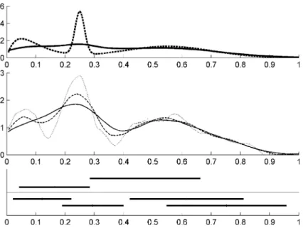
FIG. 1. Simulation for sample sizen=2000and90%-quantile.Upper display:True densityf
(dashed)and convoluted densityg(solid).Middle display:Kernel density estimates forf based on the bandwidthsh=0.22 (“ ”),h=0.31 (“ ”)andh=0.40 (“ ”).Lower display:Confidence statements.Thick horizontal lines are intervals with monotone increase/decrease(above/below the thin line).
For a sequence Nn=o(n/log3n) tending to infinity faster than log3nandun=
1/log logn, define
Bn:=
k
Nn
, l Nn
k=0,1, . . . , l=1,2, . . . ,[Nnun], k+l≤Nn .
Givenα∈(0,1), we will be able to compute boundsdt,hsuch that for all(t, h)∈
Bn, inequality (3) holds simultaneously with asymptotic probability 1−α. Taking
into account that (3) implies (4), this allows us to identify regions of increase and decrease for prescribed probability.
Figure1 shows a simulation result for n=2000, Nn= n3/5, θ=0.075 and
confidence level 90%. The upper panel of Figure1displays the true density off as well as the convoluted density g. Notice that we only have observations with densityg. In fact, by visual inspection ofgit becomes apparent how difficult it is to find segments on whichf is monotone increasing/decreasing.
not yield a contradiction, since the statement is that the monotonicity holds only on a nonempty subset of the corresponding interval. (The way the intervals are piled up in the plot, besides the fact that they are above or below the thin line, is arbitrary and does not contain information.) Recall that we have uniformity in the sense that with confidence 90% all these statements are true simultaneously; cf. also Dümbgen and Walther [13].
To illustrate our approach consider the middle panel in Figure1. Here, we have displayed three reconstructions usingt→Tt,h/(h√n)as kernel density estimator
with the same unimodal kernel as for the test statistic and three different band-widthsh∈ {0.22,0.31,0.40}. Not surprisingly (cf. Delaigle and Gijbels [10]), the reconstructions yield very different answers for what the shape off could be. For instance, focus on the left-hand side of the graph. Forh=0.22 andh=0.31, the density estimators have a mode at around 0.06, which is completely smoothed out under the larger bandwidthh=0.4. As a practitioner, not knowing the truth, we might want to screen for modes by browsing through the plots for varying band-widths and ask ourselves whether there is another mode or not. With the confidence statement in the lower display, we see that the true densityf has to have a mono-tone decrease on[0.02,0.22]with confidence 90% (this is exactly the meaning of the leftmost horizontal line). This rules out the reconstruction without a mode at 0.06, since it is monotone increasing on the whole interval[0,0.25]and thus does not reflect the right shape behavior. The kernel density estimator corresponding to the smallest bandwidth h=0.22 (although it is the best estimator in a pointwise sense) suggests that there could be another mode at around 0.58. However, since the confidence intervals do not support such a hypothesis, this could be merely an artifact. Combining the confidence statements in Figure1, we conclude that with 90% confidence the true density has a local minimum and a local maximum on
[0,1]. Repetition of the simulation shows that often two, three or four segments of increases and decreases are detected, and at most one mode on[0,1]is found (in 69% of the cases). Therefore, sample sizen=2000 is not large enough to detect systematically the correct number of minima and maxima (2 and 3). Numerical simulations for larger sample size and more details are given in Section6.
The derived confidence statements should be viewed as an additional tool for analyzing data, in particular for substantiating vague conclusions or visual impres-sions from point estimators.
1.2. Pseudo-differential operators and multiscale analysis. As mentioned at the beginning of the Introduction, we interpret shape constraints as pseudo-differential inequalities. Let F(f ) = Rexp(−ix·)f (x) dx always denote the Fourier transform of f ∈L1(R)orf ∈L2(R)(depending on the context). Con-sider a general class of differential operators op(p)with symbolp which can be written for nicef as
op(p)f(x)= 1 2π
This class will be an enlargement of (elliptic) pseudo-differential operators by frac-tional differentiation. Given data from model (1) the goal is then to identify inter-vals at a controlled error level on which Re(op(p)f )≤0 or Re(op(p)f )≥0. Here Re denotes the projection on the real part. In Section1.1we studied implicitly al-ready the case of op(p)being the differentiation operatorDf =f(monotonicity). If applied to op(p)=D2[i.e.,p(x, ξ )= −ξ2], our method yields bounds for the number and confidence regions for the location of inflection points off. We also discuss an example related to Wicksell’s problem with shape constraint described by fractional differentiation.
The statistic introduced in this paper investigates shape constraints of the un-known densityf on all scales simultaneously. Generalizing (4), we need to derive simultaneous confidence intervals for φ◦St,h,Re(op(p)f )with the
scale-and-location shiftSt,h=(· −t)/ hand the inner producth1, h2 :=
Rh1(x)h2(x) dx
inL2. If op(p) is the adjoint of op(p)(in a certain space) with respect to ·,·, then
√
nφ◦St,h,Re op(p)f
=√nRe op(p) (φ◦St,h)
(x)f (x) dx (6)
= √
n 2π Re
Fop(p) (φ◦St,h)
(s)F(f )(s) ds,
and the RHS can be estimated unbiasedly by the test statistic Tt,h :=n−1/2×
n
k=1Revt,h(Yk)with
vt,h(u):=
1 2π
Fop(p) (φ◦St,h)
(s) e
isu
F(fε)(−s)
ds.
This gives rise to a multiscale statistic
Tn=sup (t,h)
wh
|T
t,h−ETt,h|
Std(Tt,h)
−wh
,
wherewh andwh are chosen in order to calibrate the different scales with equal
weight, whileStd(Tt,h)is an estimator of the standard deviation ofTt,h.
The key result in this paper is the approximation of Tn by a distribution-free
statistic from which critical values can be inferred. Given the critical values, we can in a second step compute boundsdt,hsuch that a statement of type (3) holds.
1.3. Comparison with related work and applications. Hypothesis testing for deconvolution and related inverse problems is a relatively new area. Current meth-ods cover testing of parametric assumptions (cf. [3, 5, 29]) and, more recently, test-ing for certain smoothness classes such as Sobolev balls in a Gaussian sequence model (Laurent et al. [29, 30] and Ingster et al. [25]). All of these papers focus on regression deconvolution models. Exceptions for density deconvolution are Holz-mann et al. [23], Balabdaoui et al. [2] and Meister [33] who developed tests for various global hypotheses, such as global monotonicity. The latter test has been derived for one fixed interval and allows one to check whether a density is mono-tone on that interval at a preassigned level of significance.
Our work can also be viewed as an extension of Chaudhuri and Marron [7] as well as Dümbgen and Walther [13] who treated the case op(p)=Dm (with m=1 in [13]) in the direct case, that is, when ε=0. However, the approach in [7] does not allow for sequences of bandwidths tending to zero and yields limit distributions depending on unknown quantities again. The methods in [13] require a deterministic coupling result. The latter allows one to consider the multiscale approximation forf =I[0,1]only, but it cannot be transferred to the deconvolution
setting.
One of the main advantages of multiscale methods, making it attractive for ap-plications, is that essentially no smoothing parameter is required. The main choice will be the quantile of the multiscale statistic, which has a clear probabilistic in-terpretation. Furthermore, our multiscale statistic allows us to construct estimators for the number of modes and inflection points which have a number of nice prop-erties: First, modes and inflection points are detected with the minimax rate of convergence (up to a log-factor). Second, the probability that the true number is overestimated can be made small, since it is completely controlled by the quantile of the multiscale statistic. To state it differently, it is highly unlikely that artifacts are detected, which is a desirable property in many applications. It is worth noting that neither assumptions are made on the number of modes nor additional model selection penalties are necessary.
For practical applications, we may use these models if, for instance, the error variableε is an independent waiting time. For example let Xi be the (unknown)
time of infection of theith patient,εi the corresponding incubation time, andYi
is the time when diagnosis is made. Then, it is convenient to assumeε∼(r, θ ); see, for instance, [9], Section 3.5. By the techniques developed in this paper one will be able to identify, for example, time intervals where the number of infections increased and decreased for a specified confidence level. Another application is single photon emission computed tomography (SPECT), where the detected scat-tered photons are blurred by Laplace distributed random variables; cf. Floyd et al. [16], Kacperski et al. [27].
These results are transferred to shape constraints and deconvolution models in Sec-tion3. In Section4we discuss the statistical consequences and show how confi-dence statements can be derived. Theoretical questions related to the performance of the multiscale method and numerical aspects are discussed in Sections5and6. Proofs and further technicalities are shifted to the Appendix and a supplementary part [37].
Notation: We writeT for the set[0,1] ×(0,1]. The expression xmeans the largest integer not exceedingx. The support of a functionφis suppφ,·pdenotes
the norm in Lp:=Lp(R) and TV(·) stands for the total variation of functions onR. As customary in the theory of Sobolev spaces, puts :=(1+ |s|2)1/2. One should not confuse this with ·,·, the L2-inner product. If it is clear from the context, we writexkφandxkφfor the functionsx→xkφ(x)andx→ xkφ(x), respectively. The (L2-)Sobolev spaceHr is defined as the class of functions with norm
φHr:=
s2rF(φ)(s)2ds 1/2
<∞.
For anyqand∈N(Nis always the set of nonnegative integers) defineHq as the Sobolev type space
Hq:=ψ|xkψ∈Hq, fork=0,1, . . . ,
with normψHq :=
k=0xkψHq.
2. A general multiscale test statistic. In this section, we shall give a fairly general convergence result which is of interest on its own. The presented result does not use the deconvolution structure of model (1). It only requires that we have observationsYi=G−1(Ui), i=1, . . . , nwithUi i.i.d. uniform on[0,1]andGan
unknown distribution function with Lebesgue densitygin the class
G:=Gc,C,q :=
G|Gis a distribution function with densityg, (7)
c≤g|[0,1],g∞≤c−1,andg∈J(C, q)
for fixedc, C≥0, 0≤q <1/2 and the Lipschitz type constraint
J :=J(C, q)
:=h|h(x)−
h(y)≤C1+ |x| + |y|q|x−y|, for allx, y∈R.
For a set of real-valued functions (ψt,h)t,h define the test statistic (empirical
process) Tt,h=n−1/2nk=1ψt,h(Yk). If h is small and ψt,h localized around t,
then Std(Tt,h)≈(
ψt,h2 (s)g(s) ds)1/2 ≈ ψt,h2√g(t). It will turn out later on
that one should allow for a slightly regularized standardization, and therefore we consider
|Tt,h−E[Tt,h]|
withVt,h≥ ψt,h2 andgnan estimator ofg, satisfying
sup
G∈G
gn−g∞=OP(1/logn).
(8)
Unless stated otherwise, asymptotic statements refer ton→ ∞. We combine the single test statistics for an arbitrary subset
Bn⊂
(t, h)|t∈ [0,1], h∈ [ln, un]
(9)
and consider forν > eand
wh=
√
1/2 logν/ h log logν/ h , (10)
distribution-free approximations of the multiscale statistic
Tn:= sup (t,h)∈Bn
wh
|T
t,h−E[Tt,h]|
Vt,h
√
gn(t)
−
2 logν
h
. (11)
ASSUMPTION 1 (Assumption on test functions). Given a set Bn of the
form (9), functions(ψt,h)(t,h)∈T, and numbers(Vt,h)(t,h)∈T, suppose that the
fol-lowing assumptions hold:
(i) For all(t, h)∈T,ψt,h2≤Vt,h.
(ii) We have uniform bounds on the norms
sup
(t,h)∈T
√
hTV(ψt,h)+
√
hψt,h∞+h−1/2ψt,h1
Vt,h
1.
(iii) There existsα >1/2 such that
κn:= sup (t,h)∈Bn,G∈G
wh
TV(ψt,h(·)[√g(·)−√g(t)]·α)
Vt,h →
0.
(iv) There exists a constantKsuch that for all(t, h), (t, h)∈T,
√
h∧√h Vt,h∨Vt,h
ψt,h−ψt,h2+ |Vt,h−Vt,h|
≤K
|t−t| + |h−h|.
THEOREM1. Given a multiscale statistic of the form(11),work in model(1)
under Assumption 1, and suppose that lnnlog−3n→ ∞ and un =o(1). If the process (t, h)→√hVt,h−1ψt,h(s) dWs has continuous sample paths onT, then there exists a(two-sided)standard Brownian motionW,such that forν > e,
sup
G∈Gc,C,q
Tn− sup (t,h)∈Bn
wh
|ψ
t,h(s) dWs|
Vt,h −
2 logν
h
=OP(rn),
(12)
with
rn=sup G∈G
gn−g∞
logn log logn+l
−1/2
n n−1/2
log3/2n log logn+
√
unlog(1/un)
log log(1/un) +
Moreover,
sup
(t,h)∈T
wh
|
ψt,h(s) dWs|
Vt,h −
2 logν
h
<∞ a.s. (13)
Hence,the approximating statistic in(12)is almost surely bounded from above.
The proof of the coupling in this theorem (cf. Appendix A) is based on gener-alizing techniques developed by Giné et al. [17], while finiteness of the approx-imating test statistic utilizes results of Dümbgen and Spokoiny [12]. Note that Theorem1can be understood as a multiscale analog of theL∞-loss convergence for kernel estimators; cf. [4, 17–19].
To give an example, let us assume thatψt,h=ψ (·−ht)is a kernel function. By
Lemmas B.12 and B.4, Assumption1holds forVt,h= ψt,h2=
√
hψ2 when-everψ=0 on a Lebesgue measurable set, TV(ψ ) <∞and suppψ⊂ [0,1]. Fur-thermore, by partial integration, we can easily verify that the process (t, h)→
ψ−21ψt,h(s) dWshas continuous sample paths; cf. [12], page 144.
For an application of Theorem1to wavelet thresholding, cf. Example C.1 in the supplementary material [37]. Let us close this section with a result on the lower bound of the approximating statistic.
Theorem1shows that the approximating statistic is almost surely bounded from above. On the contrary, we have the trivial lower bound
Tn≥ − inf (t,h)∈Bn
logν/ h log logν/ h,
which converges to−∞in general and describes the behavior ofTn, provided the
cardinality ofBnis small (e.g., ifBncontains only one element). However, ifBn
is sufficiently rich,Tn can be shown to be bounded from below, uniformly in n.
Let us make this more precise. Assume, that for everynthere exists aKnsuch that
Kn→ ∞and
BK◦n := i
Kn
, 1 Kn
i=0, . . . , Kn−1 ⊂Bn.
(14)
Then the approximating statistic is asymptotically bounded from below by−1/4. This follows from Lemma C.1 in the Appendix. It is a challenging problem to cal-culate the distribution for general index setBnexplicitly. Although the tail
behav-ior has been studied for the one-scale case (cf. [4, 17]) this has not been addressed so far for the approximating statistic in Theorem1. For implementation, later on, our method relies therefore on Monte Carlo simulations.
define pseudo-differential operators in dimension one as well as fractional inte-gration and differentiation. Given a real m, consider Sm the class of functions a:R×R→Csuch that for allα, β∈N,
∂xβ∂ξαa(x, ξ )≤Cα,β
1+ |ξ|m−α for allx, ξ ∈R. (15)
Then the pseudo-differential operator Op(a)corresponding to the symbolacan be defined on the Schwartz space of rapidly decreasing functionsS by
Op(a):S→S,
Op(a)φ(x):= 1 2π
eixξa(x, ξ )F(φ)(ξ ) dξ.
It is well known that for anys∈R, Op(a)can be extended to a continuous oper-ator Op(a):Hm+s→Hs. In order to simplify the readability, we only write Op for pseudo-differential operators and op in general for operators of the form (5). Throughout the paper, we writeιαs =exp(απ isign(s)/2)and understand as usual (±is)α= |s|αι±sα. The Gamma function evaluated atα will be denoted by(α). Let us further introduce the Riemann–Liouville fractional integration operators on the real axis forα >0 by
I+αh(x):= 1 (α)
x
−∞
h(t)
(x−t)1−αdt and
(16)
I−αh(x):= 1 (α)
∞
x
h(t) (t−x)1−αdt.
For β ≥ 0, we define the corresponding fractional differentiation operators (D+βh)(x):= Dn(I+n−βh)(x) and (Dβ−h)(x) =(−D)n(I−n−βf )(x), where n= β +1. For anys∈R, we can extendDβ+andD−β to continuous operators from Hβ+s→Hsusing the identity (cf. [28], page 90)
FDβ±h(ξ )=(±iξ )βF(h)(ξ )=ι±ξβ|ξ|βF(h)(ξ ). (17)
In this paper, we consider operators op(p) which “factorize” into a pseudo-differential operator and a fractional differentiation in the Riemann–Liouville sense. More precisely, the symbolpis in the class
Sm:=(x, ξ )→p(x, ξ )=a(x, ξ )|ξ|γιμξ|a∈Sm, m=m+γ ,
γ ∈ {0} ∪ [1,∞), μ∈R.
Let us mention that we cannot allow for allγ ≥0 since in our proofs it is essential that∂ξ2p(x, ξ )is integrable. The results can also be formulated for finite sums of symbols, that is,Jj=1pj andpj ∈Sm. However, for simplicity we restrict us to
J=1.
(a1, b1), (a1, b2), (a2, b1), (a2, b2), a1< a2, b1< b2 will be denoted by[a1, a2] × [b1, b2].
The main objective of this paper is to obtain uniform confidence statement of the following kinds:
(i) The number and location of the roots and maxima of op(p)f.
(ii) Simultaneous identification of intervals of the form [ti, ti + hi], ti ∈
[0,1], hi >0, i in some index set I, with the following property: For a
pre-specified confidence level we can conclude that for all i ∈ I the functions (op(p)f )|[ti,ti+hi]attain, at least on a subset of[ti, ti+hi], positive values.
(ii) Same as (ii), but we want to conclude that(op(p)f )|[ti,ti+hi] has to attain
negative values.
(iii) For any pair(t, h)∈BnwithBnas in (9), we want to findb−(t, h, α)and
b+(t, h, α), such that we can conclude that with overall confidence 1−α, the graph of op(p)f [denoted as graph(op(p)f )in the sequel] has a nonempty intersection with every rectangle[t, t+h] × [b−(t, h, α), b+(t, h, α)].
In the following we will refer to these goals as problems (i), (ii), (ii) and (iii), respectively. Note that (ii) follows from (iii) by taking all intervals[t, t+h]with b−(t, h, α) >0. Analogously,[t, t+h]satisfies (ii) wheneverb+(t, h, α) <0. The geometrical ordering of the intervals obtained by (ii) and (ii) yields in a straight-forward way a lower bound for the number of roots of op(p)f, solving problem (i); cf. also Dümbgen and Walther [13]. A confidence interval for the location of a root can be constructed as follows: If there exists[t, t+h]such thatb−(t, h, α) >0 and
[t,t+h]withb+(t,h, α) <0, then, with confidence 1−α, op(p)f has a zero in the interval[min(t,t),max(t+h,t+h)]. The maximal number of disjoint inter-vals on which we find zeros is then an estimator for the number of roots.
EXAMPLE 1. In the example in Section1.1we had op(p)=D. In this case we want to find a collection of intervals[t, t+h]such that with overall probability 1−α for each such interval there exists a nondegenerate subinterval on whichf is strictly monotonically increasing/decreasing.
Instead of studying qualitative features of X directly, we might as well be in-terested in properties of the density of a transformed random variableq(X). IfX is nonnegative and a >0, q could be, for instance, a (slightly regularized) log-transformq=log(· +a).
EXAMPLE2. Suppose that we want to analyze the convexity/concavity prop-erties of U =q(X), where q is a smooth function, which is strictly monotone increasing on the support of the distribution ofX. LetfU denote the density ofU.
Then, by change of variables
fU(y)=
1 q(q−1(y))f
and there is a pseudo-differential operator Op(p)with symbol
p(x, ξ )= − 1 (q(x))2ξ
2−q(x)q(x)+2q(x)
(q(x))4 iξ+
3(q(x))2−q(x)q(x) (q(x))5 ,
such thatfU(y)=(op(p)f )(q−1(y)). Therefore,
graphop(p)f∩ [t, t+h] ×b−(t, h, α), b+(t, h, α)=∅
implies
graphfU∩q(t), q(t+h)×b−(t, h, α), b+(t, h, α)=∅.
In particular, ifb−(t, h, α) >0, then, with confidence 1−α, we may conclude that fU is strictly convex on a nondegenerate subinterval of[q(t), q(t+h)].
EXAMPLE 3 (Noisy Wicksell problem). In the classical Wicksell problem, cross-sections of a plane with randomly distributed balls in three-dimensional space are observed. From these observations the distributionH or densityh=H of the squared radii of the balls has to be estimated; cf. Groeneboom and Jong-bloed [21]. Statistically speaking, we have observations X1, . . . , Xnwith density
f satisfying the following relationship (cf. Golubev and Levit [20]):
1−H (x)∝ ∞
x
f (t)
(t−x)1/2dt=
1
2
I−1/2f(x) for allx∈ [0,∞),
where∝means up to a positive constant andI−1/2as in (16). Suppose now that we are interested in monotonicity properties of the densityh=Hon[0,1]. Forx >0,
−h≶0 if and only if the fractional derivative of order 3/2 satisfies(D3−/2f )(x)= D2(I−1/2f )(x)≶0. It is reasonable to assume in applications that the observations are corrupted by measurement errors, which means we only observeYi=Xi+εi
as in model (1). Hence we are in the framework described above and the shape constraint is given by op(p)f ≶0 forp(x, ξ )=ιξ−3/2|ξ|3/2.
In order to formulate our results in a proper way, let us introduce the following definitions. We say that a pseudo-differential operator Op(a)witha∈SmandSm as in (15) is elliptic if there existsξ0 such that |a(x, ξ )|> K|ξ|m for a positive
constantK and allξ satisfying|ξ|>|ξ0|. In the framework of Example2, for in-stance, ellipticity holds ifq∞<∞. It is well known that ellipticity is equivalent to a generalized invertibility of the operator. Furthermore, for an arbitrary symbol p∈Sm, let us denote by Op(p )the adjoint of Op(p)with respect to the inner product·,·. This is again a pseudo-differential operator andp ∈Sm. Formally, we can compute p by p (x, ξ )=e∂x∂ξp(x, ξ ), where p denotes the complex
we have a symbol in Sm of the form a|ξ|γιμξ =a(x, ξ )|ξ|γιμξ with a∈Sm and m+γ =m. Since for anyu, v∈Hm,
opa|ξ|γιμξu, v=Op(a)op|ξ|γιμξu, v=op|ξ|γιμξu,Opa v (18)
=u,op|ξ|γιξ−μOpa v,
we conclude thatF(op(a|ξ|γιμξ) φ)= |ξ|γι−ξμF(Op(a )φ)for allφ∈Hm. In order to formulate the assumptions and the main result, let us fix one sym-bol p∈Sm and one factorization p(x, ξ )=a(x, ξ )|ξ|γιμξ with a, γ , μas in the definition ofSm.
ASSUMPTION 2. We assume that there is a positive real number r >0 and constants 0< Cl ≤Cu<∞such that the characteristic function of ε is bounded
from below and above by
Cls−r≤Ee−isε=F(fε)(s)≤Cus−r for alls∈R.
Moreover, suppose that the second derivative ofF(fε)exists and
sDF(fε)(s)+ s2D2F(fε)(s)≤Cus−r for alls∈R.
These are the classical assumptions on the decay of the Fourier transform of the error density in the moderately ill-posed case; cf. Assumptions (G1) and (G3) in Fan [15]. Heuristically, we can think ofF(fε)as an elliptic symbol inS−r.
Let Re denote the projection on the real part. For sufficiently smoothφconsider the test statistic
Tt,h:=
1
√
n
n
k=1
Revt,h(Yk)=
1
√
n
n
k=1
Revt,h
G−1(Uk)
(19)
with
vt,h=F−1
λμγ(·)FOpa (φ◦St,h)
(20)
and
λ(s)=λμγ(s)= |s|
γι−μ s F(fε)(−s)
. (21)
From (6) and (18), we find that forf ∈Hm,
ETt,h=
√
n
(φ◦St,h)(x)Re
op(p)f(x) dx.
Proceeding as in Section2we consider the multiscale statistic
Tn= sup (t,h)∈Bn
wh
|T
t,h−E[Tt,h]|
√
gn(t)vt,h2
−
2 logν
h
that is, with the notation of (11), we setψt,h:=Revt,handVt,h:= vt,h2. Define
further
Tn∞(W ):= sup
(t,h)∈Bn
wh
|Rev
t,h(s) dWs|
vt,h2
−
2 logν
h
.
THEOREM 2. Given an operator op(p) with symbol p∈ Sm, let Tn be as in(22).Work in model(1)under Assumption2.Suppose that:
(i) lnnlog−3n→ ∞andun=o(log−3n);
(ii) φ∈H4r+m+5/2, suppφ⊂ [0,1],andTV(D r+m+5/2φ) <∞; (iii) Op(a)is elliptic.
Then there exists a(two-sided)standard Brownian motionW,such that forν > e,
sup
G∈Gc,C,q
Tn−Tn∞(W )=oP(rn),
(23)
with
rn=sup G∈G
gn−g∞
logn log logn+l
−1/2
n n−1/2
log3/2n log logn+u
1/2
n log3/2n.
Moreover,
sup
(t,h)∈T
wh
|Rev
t,h(s) dWs|
vt,h2 −
2 logν
h
<∞ a.s. (24)
Hence the approximating statisticTn∞(W ) is almost surely bounded from above by(24).
One can easily show using Lemma C.1, that ifBn contains (14) and the
sym-bolp does not depend ont, then the approximating statistic is also bounded from below. Furthermore, the caseε=0 can be treated as well [we can defineF(fε)=1
in this case]. In particular, our framework allows for the important caseε=0 and op(p)the identity operator, which cannot be treated with the results from [13].
For special choices of p and fε the functions (vt,h)t,h have a much simpler
form, which allows us to read off the ill-posedness of the problem from the in-dex of the pseudo-differential operator associated withvt,h. Let us shortly discuss
this. Suppose Assumption 2holds and additionally sk|DkF(fε)(s)| ≤Cks−r
for alls∈Randk=3,4, . . . .Then(x, ξ )→F(fε)(−ξ )defines a symbol inS−r.
Because of the lower bound in Assumption2,Clξ−r ≤ |F(fε)(−ξ )|, the
corre-sponding pseudo-differential operator is elliptic, and(x, ξ )→1/F(fε)(−ξ )is the
symbol of a parametrix and consequently an element inSr; cf. Hörmander [24], Theorem 18.1.9. Ifφ∈Hr+mandp∈Sm∩Sm, then
vt,h(u)=
1 2π F Op 1
F(fε)(−·)
◦Opp (φ◦St,h)
(s)eisuds
=Op
1
F(fε)(−·)
Pseudo-differential operators are closed under composition. More precisely,pj ∈
Smj forj =1,2 implies that the symbol of the composed operator is inSm1+m2. Therefore, there is a symbol p∈Sm+r such that vt,h=Op(p)(φ◦St,h). Hence,
for fixedh, the functiont→vt,hcan be viewed as a kernel estimator with
band-width h. Furthermore, the problem is completely determined by the composition Op(p), and this yields a heuristic argument as to why (as it will turn out later) the ill-posedness of the detection problem Re op(p)f ≶0 in model (1) is determined by the summ+r, that is,
ill-posedness of shape constraint+ill-posedness of deconvolution problem.
Suppose further thatr andmare integers, and Op(p)is a differential operator of the form
m
k=1
ak(x)Dk
(25)
with smooth functionsakk=1, . . . , mandambounded uniformly away from zero.
If 1/F(fε)(−·)is a polynomial of degreer (which is true, e.g., ifεis Exponential,
Laplace or Gamma distributed), then Op(p) is again of the form (25) but with degreem+r, and hencevt,h(u)is essentially a linear combination of derivatives
ofφ evaluated at(u−t)/ h. However, these assumptions on the error density are far to restrictive. In the following paragraph we will show that even under more general conditions the approximating statistic has a very simple form.
Principal symbol. In order to perform our test, it is necessary to compute quan-tiles of the approximating statistic in Theorem2. Since the approximating statistic has a relatively complex structure let us give conditions under which it can be simplified considerably. First, we impose a condition on the asymptotic behavior of the Fourier transform of the errors. Similar conditions have been studied by Fan [14] and Bissantz et al. [4]. Recall that for any α, a∈R, s=0, Dιαs|s|a = D(is)a1(−is)a2=aiια−1
s |s|a−1witha1=(a+α)/2 anda2=(a−α)/2.
ASSUMPTION 3. Suppose that there exist β0 >1/2, ρ∈ [0,4) and positive
numbersA, Cεsuch that
AιρssrF(fε)(s)−1+Ar−1iιsρ+1|s|r+1DF(fε)(s)−1≤Cεs−β0
∀s∈R.
For instance the previous assumption holds withA=θr andρ≡rmod 4 iffε
is the density of a (r, θ ) distributed random variable. In this case F(fε)(s)=
ASSUMPTION4. Givenm= {0} ∪ [1,∞), suppose there exists a decomposi-tionp=pP +pRsuch thatpR∈Sm
for somem< m, and
pP(x, ξ )=aP(x)|ξ|mιμξ for allx, ξ∈R,
with(x, ξ )→aP(x)∈S0,aP real-valued and|aP(·)|>0.
Fors=0,ι2s= −1. Assume that in the special casem=0 we have|ρ+μ| ≤r. Then, we can (and will) always chooseρandμin Assumptions3and4such that σ=(r+m+ρ+μ)/2 andτ =(r+m−ρ−μ)/2 are nonnegative. The symbol pP is called principal symbol. We will see that, together with the characteristics
from the error density, it completely determines the asymptotics. The condition basically means that there is a smooth functionbsuch that the highest order of the pseudo-differential operator coincides withaP(x)Dm. Note that principal symbols
are usually defined in a slightly more general sense; however Assumption4turns out to be appropriate for our purposes. In particular, the last assumption is verified for Examples1–3.
In the following, we investigate the approximation of the multiscale test statistic
TnP := sup
(t,h)∈Bn
wh
hr+m−1/2|T
t,h−E[Tt,h]|
√
gn(t)|AaP(t)|D+r+mφ2
−
2 logν
h
, (26)
by
TnP ,∞(W ):= sup
(t,h)∈Bn
wh
|Dσ
+D−τφ((s−t)/ h) dWs|
D+r+mφ((· −t)/ h)2 −
2 logν h
.
THEOREM3. Work under Assumptions2,3and4.Suppose further,that
(i) lnnlog−3n→ ∞andun=o(log−(3∨(m−m
)−1) n);
(ii) φ∈H3r+m+5/2, suppφ⊂ [0,1]TV(D r+m+5/2φ) <∞; (iii) ifm=0,assume thatr >1/2and|μ+ρ| ≤r.
Then there exists a(two-sided)standard Brownian motionW,such that forν > e,
sup
G∈Gc,C,q
TP
n −TnP ,∞(W )=oP(1),
and the approximating statisticTnP ,∞(W )is almost surely bounded from above by
sup
(t,h)∈T
wh
|Dσ
+D−τφ((s−t)/ h) dWs|
D+r+mφ((· −t)/ h)2 −
2 logν h
4. Confidence statements.
4.1. Confidence rectangles. Suppose that Theorem2holds. The distribution ofTn∞(W )depends only on known quantities. By ignoring theoP(1)term on the
right-hand side of (23), we can therefore simulate the distribution ofTn. To
for-mulate it differently, the distance between the(1−α)-quantiles ofTnandTn∞(W )
tends asymptotically to zero, althoughTn∞(W )does not need to have a weak limit. The(1−α)-quantile ofTn∞(W )will be denoted byqα(Tn∞(W ))in the sequel.
In order to obtain a confidence band one has to control the bias which requires a Hölder condition on op(p)f. However, since we are more interested in a qual-itative analysis, it suffices to assume that op(p)f is continuous [andf ∈Hm in order to define the scalar product of op(p)f properly]. Moreover, instead of a mo-ment condition on the kernelφ, we require nonnegativity, that is, for the remaining part of this work, assume thatφ≥0 andφ(u) du=1. Theorem2 implies that asymptotically with probability 1−α, for all(t, h)∈Bn,
φt,h,op(p)f
∈
T
t,h−dt,h
√
n ,
Tt,h+dt,h
√ n , (28) where
dt,h:=
gn(t)vt,h2
2 logν
h
1+qα
Tn∞(W )log logν/ h logν/ h
.
Using the continuity of op(p)f, it follows that asymptotically with confidence 1−α, for all(t, h)∈Bn, the graph ofx→op(p)f (x)has a nonempty intersection
with each of the rectangles
[t, t+h] ×
Tt,h−dt,h
h√n ,
Tt,h+dt,h
h√n
. (29)
This means we find a solution of (iii) by setting
b−(t, h, α):= Tt,h−dt,h
h√n , b+(t, h, α):=
Tt,h+dt,h
h√n . (30)
If instead Theorem3holds, we obtain by similar arguments that asymptotically with confidence 1−α, for all (t, h)∈Bn, the graph of x →op(p)f (x) has a
nonempty intersection with each of the rectangles
[t, t+h] × T
t,h−dt,hP
h√n ,
Tt,h+dt,hP
h√n (31)
with
dt,hP :=
gn(t)AaP(t)h1/2−m−rD+r+mφ2
2 logν
h (32)
×
1+qα
TnP ,∞(W )log logν/ h logν/ h
andqα(TnP ,∞(W ))the 1−α-quantile ofTnP ,∞(W ). Therefore we find a solution
with
b−(t, h, α):= Tt,h−d
P t,h
h√n , b+(t, h, α):=
Tt,h+dt,hP
h√n .
Finally let us mention that instead of rectangles we can also cover op(p)f by ellipses. Note that in particular a rectangle is an ellipse with respect to the · ∞ vector norm on R2, that is, (up to translation) a set of the form
{(x1, x2): max(a|x1|, b|x2|)=1}for positivea, b.
4.2. Comparison with confidence bands. Let us shortly comment on the re-lation between confidence rectangles and confidence bands, which for density de-convolution were studied by Bissantz et al. [4] and Lounici and Nickl [31]. Fix one scaleh=hnand consider Bn= [0,1] × {h}. For simplicity let us further restrict
to the framework of Theorem2. From (28), we obtain that
t→
Tt,h−dt,h
h√n ,
Tt,h+dt,h
h√n (33)
is a uniform (1−α)-confidence band for the locally averaged function t →
1
hφt,h,op(p)f. Restricting to scales on which the stochastic error dominates the
bias |op(p)f − 1hφt,h,op(p)f| (e.g., by slightly undersmoothing) we can,
in-flating (33) by a small amount, easily construct asymptotic confidence bands for op(p)f as well. Note that Theorem2does not require thatsrF(fε)(s)converges
to a constant, and therefore we can construct confidence bands for situations which are not covered within the framework of [4]. However, the construction of confi-dence bands described above will not work on scales where we oversmooth or if bias and stochastic error are of the same order. The strength of the multiscale ap-proach lies in the fact that for confidence rectangles, all scales can be used simulta-neously. This allows for another view on confidence rectangles. Figure2displays a band (33) computed for a large scale/bandwidth which obviously does not cover op(p)f. Now, take a point,t0say, then (29) is equivalent to the existence of a point
t0 ∈ [t0, t0+h]such that the confidence interval[A, B]att0shifted tot0 (and
de-noted by [A, B] in Figure 2) contains op(p)f (t0). Thus, confidence rectangles also account for the uncertainty oft→op(p)f (t)along thet-axis.
5. Choice of kernel and theoretical properties of the multiscale statistic.
In this section, we investigate the size/area of the rectangles constructed in the pre-vious paragraphs. Recall that by (6) the expectation of the statisticTt,hdepends in
general on op(p). In contrast, Theorem3shows that the variance ofTt,hdepends
FIG. 2. Obtaining confidence rectangles from bands.
5.1. Optimal choice of the kernel. In what follows we are going to study the problem of finding an optimal functionφ. Ifm+r ∈Nand the confidence state-ments are formulated via the conclusions of Theorem3, this can be done explicitly. Note that for given (t, h) ∈ Bn, the width of rectangle (31) is given by
2dt,hP /(h√n). Further, the choice of φ influences the value of dt,hP in two ways, namely by the factor D+r+mφ2 = Dr+mφ2 as well as the quantile qα(TnP ,∞(W )); cf. the definition ofdt,hP given in (32). Sinceαis fixed, we have
qα
TnP ,∞(W )log logν/ h
logν/ h =o(1).
Therefore,dt,hP depends in first order onDr+mφ2 and our optimization problem can be reformulated as
minimizeDr+mφ2 subject to
φ(u) du=1.
This is in fact easy to solve if we additionally assume thatφ ∈Hq withr +m≤ q < r+m+1/2. By Lagrange calculus, we find that on (0,1), φ has to be a polynomial of order 2m+2r. Under the induced boundary conditionsφ(k)(0)= φ(k)(1)=0 fork=0, . . . , r+m−1, the solutionφm+r is of the form
φm+r(x)=cm+rxm+r(1−x)m+rI(0,1)(x).
(34)
Due to the normalization constraintφm+r(u) du=1, it follows thatφm+r is the
density of a beta distributed random variable with parametersα=m+r+1 and β=m+r +1, implying, cm+r=(2m+2r+1)!/((m+r)!)2. It is worth
the(m+r)th Legendre polynomialLm+r, that is,
φm(m++rr)=(−1)m+r(2m+2r+1)!
(m+r)! Lm+r(2· −1)
(this is essentially Rodrigues’s representation; cf. Abramowitz and Stegun [1], page 785). For that reason, we even can compute
φ(m+r) m+r L2=
(2m+2r)! (m+r)!
√
2m+2r+1.
In the particular case ofr=0, m=1 we obtainφ1(1)(x)∝1−2x. This is known from the work of Dümbgen and Walther [13] who considered locally most power-ful tests to deriveφ1(1).
To summarize, we can find the “optimal” kernel, but it turns out that it has less smoothness than it is required by the conditions for Theorem3 due to its behavior on the boundaries {0,1}. However, if the operator defining the shape constraint and the inversion operatorg→f are both differential operators (for an example see Section1.1), then the theorems can be proved under weaker assumptions onφ including as a special case the optimal beta kernels.
5.2. Theoretical properties of the method. In this part, we give some theoret-ical insights. We start by investigating problem (iii); cf. Section3. After that, we will address issues related to (ii) and (i). It is easy to see thatvt,h2h1/2−m−r,
and thusdt,h and dt,hP are of the same order. We can therefore restrict ourselves
in the following to the situation, where the confidence statements are constructed based on the approximation in Theorem2. In the other case, similar results can be derived.
Problem(iii): Recall that with confidence 1−α, for all(t, h)∈Bn,
graphop(p)f∩ [t, t+h] × T
t,h−dt,h
h√n ,
Tt,h+dt,h
h√n
=∅.
The so constructed rectangles localize op(p)f, where the amount of information is directly linked to the size of the rectangle. Therefore, it is natural to think of the length of the diagonal as a measure of localization quality. This length behaves likeh∨h−m−r−1/2n−1/2√log 1/ h. In particular, if the rectangle is a square, then h∼(logn/n)1/(3+2m+2r), and this coincides with the optimal bandwidth for a kernel density estimator under a Lipschitz assumption onf. This is no surprise, of course, since Lipschitz continuity allows a function to oscillate over an intervalI by an amount that is proportional to the length|I|.
Problem(ii), (ii): The following lemma gives a necessary condition in order to solve (ii). Loosely speaking, it states that whenever
op(p)f|[t,t+h]n−1/2h−m−r−1/2
the multiscale test returns a rectangle[t, t+h] × [b−(t, h, α), b+(t, h, α)]which is in the upper half-plane with high-probability. Or, to state it differently, we can reject that op(p)f|[t,t+h]<0.
In order to formulate the next theorem, recall the definition ofb±(t, h, α)given in (30). Further, set rt,h,n:=2dt,h/(h
√
n) and denote by Mn− the set of tupels (t, h)∈Bn for which op(p)f|[t,t+h] > rt,h,n. Similarly define Mn+:= {(t, h)∈
Bn|op(p)f|[t,t+h]<−rt,h,n}.
THEOREM4. Work under the assumptions of Theorem2.Ifφ≥0,then
lim
n→∞P
(−1)∓b±(t, h, α) >0, for all(t, h)∈Mn±≥1−α.
PROOF. For all(t, h)∈Mn−, conditionally on the event given by (28),
op(p)f|[t,t+h]> rt,h,n⇒
φt,h,op(p)f
> hrt,h,n,
⇒Tt,h> dt,h⇒b−(t, h, α) >0.
One can argue similarly forMn+.
Define
Cα:=
8fε∞hm+r−1/2vt,h2
1+qα
Tn∞(W )2/(2m+2r+1), (35)
and letM±be the set of tupels(t, h)∈Bnsatisfying the pair of constraints
h≥Cα
logn
n
1/(2β+2m+2r+1)
and
op(p)f|[t,t+h]≶
logn
n
β/(2β+2m+2r+1)
(36)
(with>in the last equality corresponding toMn−and<toMn+).
COROLLARY1. Work under the assumptions of Theorem2.Ifφ≥0andβ∈ R,then
lim
n→∞P
(−1)∓b±(t, h, α) >0, for all(t, h)∈Mn±≥1−α.
PROOF. It holds that
dt,h≤ fε1∞/2vt,h2
2 logν/ h1+qα
Tn∞(W ).
For sufficiently largen,h≥ln≥ν/n. Therefore we have for every(t, h)∈Mn−,
rt,h,n≤
8fε∞vt,h2
1+qα
Tn∞(W )h−1/2n−1/2
and similarly for Mn+. Since Mn±⊂Mn±, the result follows directly from Theo-rem4.
Roughly speaking, the last result shows that ifh∼(logn/n)1/(2β+2m+2r+1)and op(p)f|[t,t+h]∼(logn/n)β/(2β+2m+2r+1)=hβ, then with probability 1−α, our
method returns a rectangle in the upper half-plane. We have three distinct regimes,
β >0 : op(p)f|[t,t+h]→0,
β=0 : op(p)f|[t,t+h]=O(1),
−m−r−12 < β <0 : op(p)f|[t,t+h]→ ∞.
It is insightful to compare the previous result to derivative estimation of a density ifm+r is a positive integer. As it is well known, Dm+rf can be estimated with rate of convergence
logn
n
β/(2β+2m+2r+1)
under L∞-risk assuming that op(p)f is Hölder continuous with index β > 0 andh∼(logn/n)1/(2β+2m+2r+1). This directly relates to the first case considered above.
Problem(i): At the beginning of Section3we shortly addressed construction of confidence statements for the number of roots and their location. Note that estima-tors derived in this way have many interesting features. On the one hand, we know that with probability 1−α the estimated number of roots is a lower bound for the true number of roots. Therefore, these estimates do not come from a trade-off between bias and variance, but they allow for a clear control on the probability to observe artifacts. In order to show that the lower bound for the number of roots is not trivial, we need to prove that whenever two roots are well separated (e.g., the distance between them does not shrink too quickly), they will be detected even-tually by our test. This property follows if we can show that the simultaneous confidence intervals for a fixed number of roots, say, shrink to zero.
Therefore, assume for simplicity that the number K and the locations (x0,j)j=1,...,K of the zeros of op(p)f are fixed (but unknown) andx0,j∈(0,1)for
j=1, . . . , K. For example, these roots can be extreme/saddle points if op(p)=D or points of inflection if op(p)=D2.
In order to formulate the result, we need thatBnis sufficiently rich. Therefore,
we assume that for alln, there exists a sequence(Nn), Nnn1/(2m+2r+1)log4n,
such that
k
Nn
, l Nn
k=0,1, . . . , l=1,2, . . . , k+l≤Nn ⊂Bn.
Assume further that in a neighborhood of the rootsx0,j, op(p)f behaves like
op(p)f (x)=γsign(x−x0,j)|x−x0,j|β+o
|x−x0,j|β
for some positive β ∈ (0,1]. Let ρn = (logn/n)1/(2β+2m+2r+1)2/γ1/β and
Cα, Mn± as defined in Corollary 1. There exist integer sequences (kj,n− )j,n,
(k+j,n)j,n,(ln)nsuch that for all sufficiently largen,
ρn≤
kj,n−
Nn −
x0,j≤2ρn, −2ρn≤
k+j,n
Nn −
x0,j≤ −ρn
and
Cαγ1/βρn≤
ln
Nn ≤
2Cαγ1/βρn.
Direct calculations show (kj,n− /Nn, ln/Nn)∈Mn− and((kj,n+ −ln)/Nn, ln/Nn)∈
Mn+forj=1, . . . , K. We can conclude from Corollary1and the construction that forj =1, . . . , K, the confidence intervals have to be a subinterval of
k+
j,n−ln
Nn
,k
−
j,n+ln
Nn
.
Hence, the length for each confidence interval is bounded from above by
4Cαγ1/β+1
ρn∼
logn
n
1/(2β+2m+2r+1)
.
As n→ ∞ the confidence intervals shrink to zero and will therefore become disjoint eventually. This shows that our estimator for the number of roots picks asymptotically the correct number with high probability. Observe, that for local-ization of modes in density estimation (m, r, β)=(1,0,1) the rate (logn/n)1/5 is indeed optimal up to the log-factor; cf. Hasminskii [22]. The rate(logn/n)1/7 for localization of inflection points in density estimation(m, r, β)=(2,0,1) coin-cides with the one found in Davis et al. [8].
For the special case of mode estimation in density deconvolution [here (m, r, β)= (1, r,1)], let us shortly comment on related work by Rachdi and Sabre [36] and Wieczorek [39]. In [39] optimal estimation of the mode under relatively restrictive conditions on the smoothness off is considered. In contrast, Rachdi and Sabre find the same rates of convergencen−1/(2r+5)(but with respect to the mean-square error). Under the stronger assumption that D3f exists they also provide confidence bands which converge at a different rate, of course.
One of the restrictions of our method, compared to other works on multiscale statistics, is that we exclude the coarsest scales, that is, h > un=o(1); cf.
Theo-rem1. Otherwise the approximating statistic would not be distribution-free. How-ever, excluding the coarsest scales is a very weak restriction since the important features of op(p)f can be already detected at scales tending to zero with a certain rate. For instance in view of Corollary1, the multiscale method detects a devia-tion from zero, that is, op(p)f|I ≥C >0, provided the length of the intervalI
is larger than const.×(logn/n)1/(2m+2r+1). This can be also seen by numerical simulations, as outlined in the next section.
6. Numerical simulations. In this section we provide further simulation results and discussion to the example from Section 1.1 (cf. also Example 1, Section 3), that is, studying monotonicity of the density f under Laplace-deconvolution. More precisely, the error density isfε(x)=θ−1e−|x|/θ with θ =
0.075. In this case,
F(fε)(t)= θ t−2 and op(p) f = −Df.
One should notice that for Laplace deconvolution the inversion operator, map-ping g to f, is given by 1−θ2D2 and therefore statistic (19) takes the sim-ple form (2); cf. also the discussion following Theorem 2. The ill-posedness of the shape constraint and the deconvolution problem givem=1, r=2.Together with (34) it is therefore natural to chooseφ as the density of a Beta(4,4)random variable. Further, recall thatun=1/log logn,Nn= [n3/5]and
Bn=
k
Nn
, l Nn
k=0,1, . . . , l=1,2, . . . ,[Nnun], k+l≤Nn .
Note that Assumptions3and4hold for(A, ρ, r, β0)=(θ2,0,2,2)and(μ, m)=
(1,1), respectively. Thus, we might work in the framework of Theorem 3. The multiscale statistics
TnP = sup
(t,h)∈Bn
wh
|T
t,h−ETt,h|
√
gn(t)θ2φ(3)2
−
2 log
ν
h
and
TnP ,∞(W )= sup
(t,h)∈Bn
wh
|φ(3)((s−t)/ h) dW s|
√
hφ(3)2 −
2 log
ν
h (37)
have a particular simple form as well, and the rectangles in (31) can be computed via
dt,hP =h−5/2
gn(t)θ2φ(3)2
2 logν
h
1+qα,n
log logν/ h logν/ h
. (38)
FIG. 3. Boxplots for three different values(n=200, n=1000, n=10,000)of the approximating statistic(37).
well-concentrated with a few outliers only. Although our theoretical results imply boundedness of the multiscale statistic asn→ ∞, Figure3indicates that ifnis in the range of a few thousand,TnP ,∞(W )increases slowly.
In Section1.1we showed confidence statements for a simulated sample of size n=2000. To complement our study, let us now investigate the case of largen, that is,n=10,000. Again we choose the confidence level equal to 90%. The estimated quantile isq0.1(T10P ,,000∞ (W ))= −0.04. For all simulations, we useν=exp(e2)
be-cause then h→√logν/ h/(log logν/ h) is monotone as long as 0< h≤1; cf. Lemma B.11(i). The densityf has been designed in order to investigate Corollary
1numerically. Indeed, on[0,0.35] the signal|f|is large on average, but the in-tervals on whichf increases/decreases are comparably small. By way of contrast, on[0.35,1]the signal|f|is small and there is only one increase/decrease.
The test is able to find all increases and decreases of f besides the increase on [0,0.04], which is not detected; cf. Figure 4. In contrast to the simulation in
FIG. 4. Simulation for sample sizen=10,000and90%-quantile.Upper display:True densityf
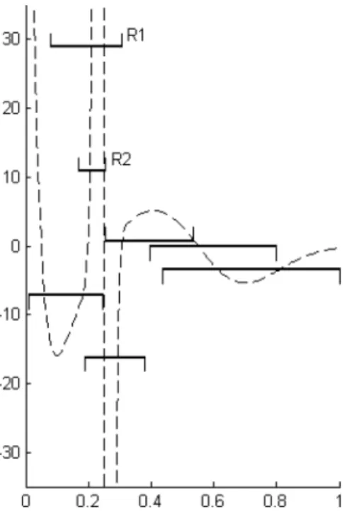
FIG. 5. True(unobserved)derivativef (dashed)and confidence statements for the level off.
Computed for the same data set as in Figure4.
Figure1, we see now a much better localization of the sharp increase/decrease on
[0.2,0.25]and[0.25,0.3].
With the confidence rectangles at hand, we are able to say more aboutf than localizing regions of increase/decrease only. In fact, we also can provide some con-fidence statements about the value offclose to a given point. Instead of plotting all confidence statements, we have displayed in Figure5the most prominent ones, allowing for a good characterization of the derivativef and telling us something about the strength of the increases/decreases off.
A bracket of type “” means thatf has to be above the horizontal line, some-where. To give an example, from the bracket R1 we can conclude that at least on a subset of[0.07,0.3], the derivativefexceeds 29. Similarly, “” means that somewherefhas to be below the corresponding horizontal line. As always, these statements hold simultaneously with confidence 90%.
What we find is that in regions where the derivative does not oscillate much, we can achieve rather precise confidence statements about the value of f. For example, from the rightmost bracket we can infer that with 90% confidence, the minimum off on [0.45,1] has to be below−4, coming close to the true mini-mum, which is approximately−6.