Procedia Computer Science 57 ( 2015 ) 772 – 781
1877-0509 © 2015 The Authors. Published by Elsevier B.V. This is an open access article under the CC BY-NC-ND license (http://creativecommons.org/licenses/by-nc-nd/4.0/).
Peer-review under responsibility of organizing committee of the 3rd International Conference on Recent Trends in Computing 2015 (ICRTC-2015) doi: 10.1016/j.procs.2015.07.474
ScienceDirect
3rd International Conference on Recent Trends in Computing 2015 (ICRTC-2015)
Empirical Validation of Neural Network Models for Agile Software
Effort Estimation based on Story Points
Aditi Panda, Shashank Mouli Satapathy*, Santanu Kumar Rath
Department of Computer Science and Engineering,National Institute of Technology Rourkela, Rourkela, Odisha – 769008, India
Abstract
Now-a-days agile software development process has become famous in industries and substituting the traditional methods of software development. However, an accurate estimation of effort in this paradigm still remains a dispute in industries. Hence, the industry must be able to estimate the effort necessary for software development using agile methodology efficiently. For this, different techniques like expert opinion, analogy, disaggregation etc. are adopted by researchers and practitioners. But no proper mathematical model exists for this. The existing techniques are ad-hoc and are thus prone to be incorrect. One popular approach of calculating effort of agile projects mathematically is the Story Point Approach (SPA). In this study, an effort has been made to enhance the prediction accuracy of agile software effort estimation process using SPA. For doing this, different types of neural networks (General Regression Neural Network (GRNN), Probabilistic Neural Network (PNN), Group Method of Data Handling (GMDH) Polynomial Neural Network and Cascade-Correlation Neural Network) are used. Finally performance of the models generated using various neural networks are compared and analyzed.
© 2015 The Authors. Published by Elsevier B.V.
Peer-review under responsibility of organizing committee of the 3rd International Conference on Recent Trends in Computing 2015 (ICRTC-2015).
Keywords: Agile Software Development; General Regression Neural Network; Probabilistic Neural Network; GMDH Polynomial Neural Network; Cascade Correlation Neural Network; Software Effort Estimation; Story Point Approach
* Corresponding author. Tel.: +91 – 661 – 246 - 4356
E-mail address: [email protected]
© 2015 The Authors. Published by Elsevier B.V. This is an open access article under the CC BY-NC-ND license (http://creativecommons.org/licenses/by-nc-nd/4.0/).
Peer-review under responsibility of organizing committee of the 3rd International Conference on Recent Trends in Computing 2015 (ICRTC-2015)
1.Introduction
Agile methods are used while developing software to enable organizations respond to volatility. They provide chances to evaluate the direction all through the software development life cycle (Fowler1). By emphasizing on the repetition of work cycles along with product the teams yield an additive and iterative development. Instead of promising to market an assemble software that hasn't been developed, agile authorizes teams to repetitively re-plan their release to optimize its value throughout development (Schmietendorf3), in the marketplace making them competitor (Cohen5, PopliISCON23).
Since predictability is the primary goal of project management, we need to be able to estimate the size and complexity of the products to be built in order to determine what to do next (SatapathyFCPASPRINGER20136, SatapathyACMSIGSEN12). For this, requirements need to be collected. Requirements in agile development are jotted down in cards and are called user stories. These stories are estimated using story points. The team defines the relationship between story point and effort. Usually 1 story point is equal to 1 ideal working day. Total no. of story points that a team can convey in a sprint (an iteration in agile software development) is called as “team velocity” or story points per sprint. In the SPA, aggregate number of story points alongside velocity of the project are considered to determine agile software development effort. Now for obtaining better prediction accuracy, four different neural network techniques are used in this study. The results obtained by applying these networks are empirically validated and compared to assess their performance.
2.Related Work
Keaveney et al. (Keaveney7) investigated the pertinence of conventional effort estimation procedures towards agile software development approaches. Coelho et al. (Coelho8) described the steps followed in story point-based method for effort estimation of agile software and highlighted the areas which need to be looked into further research. Andreas Schmietendorf et al. (Schmietendorf3) provided an investigation about estimation possibilities, especially for the extreme programming paradigm. Ziauddin et al. (Zia9) developed an effort estimation model for agile software projects. The model was fine-tuned with the help of the empirical data acquired from twenty one software projects. The test results demonstrate that model has great estimation exactness regarding MMRE and PRED(n). Satapathy et al. used SVR-Kernel methods for optimizing the effort calculated using story point approach in SatapathySPASEKE20142. Out of the four kernels used, the RBF-Kernel is shown to have best accuracy. Popli et al. (PopliICROIT14) proposed a model for effort and cost estimation in agile software development by using regression analysis. This framework is suitable to be used for project planning, execution and monitoring efficaciously. Hussain et al. (Hussain15) made an attempt to propose an approach which helps in removing problems like formalized user requirements and thus apply function points for agile software effort estimation. Hamouda et al. (Hamouda16) introduced a process and methodology that guarantees relativity in software sizing while using agile story points.
Parag C. Pendharkar (PendharkarElSVJ201024) also proposed a PNN approach for predicting a software development parameter and a probability measure which denotes the chances of actual value of the parameter being less than its estimated value at the same time. This PNN approach was then compared with Chi-squared Automatic Interaction Detection (CHAID). Results indicate that PNN performs similar to the CHAID, but provides superior probability estimates. P. Reddy et al. (Reddy21) proposed software effort estimation models based on Radial Basis Function Neural Network (RBFN) and GRNN. Results proved that RBFN performs better than GRNN. P. S. Rao et al. (Rao22) proposes a GRNN to utilize improved software effort estimation for COCOMO dataset. The GRNN model is then compared with various other techniques, i.e., M5, Linear regression, SMO Poly-kernel and RBF kernel. Fahlman et al. (fahlman19) first proposed the cascade-correlation learning architecture for artificial neural networks. They are self-organizing networks, starting only with input and output neurons and adding hidden-layer neurons during the training process. The GMDH neural networks are illustrated by Farlow et al. in (farlow20) but they were first developed in the Combined Control Systems (CCS) group of the Institute of Cybernetics in Kyiv (Ukraina) in 1968. They are also self-organizing, starting only with input neurons and adding hidden units during training based on some criteria.
3.Evaluation criteria
The performance of the various models is accessed by employing criteria outlined below (Menzies13): x The Mean Square Error (MSE) is calculated as:
ܯܵܧ ൌ ሺσ
்ୀଵሺܣܧ
െ ܲܧ
ሻ
ଶሻ ܶܦ
Τ
(1)Where AEi = Actual Effort of ith test data, PEi = Predicted Effort of ith test data and TD = Total number of data in the test set.
x The squared correlation coefficient (R2), otherwise called as the coefficient of determination is calculated as:
ܴ
ଶൌ ͳ െ ሺሺσ
்ୀଵሺܣܧ
െ ܲܧ
ሻ
ଶሻ ሺσ
Τ
்ୀଵሺܣܧ
െ ܣܧሻ
ଶሻሻ
(2)Where AE = Mean of Actual Effort Value.
x The Mean Magnitude of Relative Error (MMRE) is calculated by summing MRE values over N observations:
ܯܯܴܧ ൌ σ
்ሺȁܣܧ
െ ܲܧ
ȁ
ୀଵ
Τ
ܣܧ
ሻ
(3)
x The Prediction Accuracy (PRED) is calculated as:
ܴܲܧܦ ൌ ሺͳ െ ቀሺσ
்ୀଵሺȁܣܧ
െ ܲܧ
ȁ
ሻ ܶܦ
Τ
ሻቁሻ כ ͳͲͲ
(4)
4.Proposed work
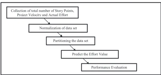
The proposed approach is implemented using the twenty one project data set developed by six software houses (Zia9). The data set is three-dimensional. The first dimension indicates the number story points required to complete the project, the second represents the velocity of the project, and the third represents the actual effort required to complete that project. This data is used by (Zia9) for predicting effort using regression. In this study, in order to enhance the effort estimation accuracy, neural networks are employed. The block diagram, demonstrated in figure 1, shows the proposed steps applied to predict effort with the help of various neural network models.
The steps taken to determine the effort of a software product are described below:
x Collection of Total Number of Story Points, Project Velocity and Actual Effort: The total number of story points, project velocity values and actual effort are collected from (Zia9).
x Normalization of Data Set: This step deals with generating the normalized values of the total number of story points and project velocity within the range [0,1]. Let Y be the complete data set and y is an element of the data set, then the normalized value of y can be calculated as:
ݕᇱൌ ሺݕ െ ሺݕሻሻ ሺሺݕሻ െ ሺݕሻሻΤ (5)
where y' = Normalized value of y in the range [0,1], min(Y) = minimim value of Y and max(Y) = maximum value of Y. When max(Y) = min(Y), y' = 0.5.
x Partitioning the Data Set: The complete data set is partitioned into training set and test set.
x Predict the effort value: The GRNN and PNN algorithms are run to get effort values. No network building is involved as everything is decided before making the effort prediction. In case of self-organizing
networks, the values of learning parameters are assigned and the algorithm is run until an optimum network configuration is obtained.
x Performance Evaluation: In this step, the models are accessed in order to evaluate their performance using MSE, R2, MMRE, Prediction Accuracy (PRED) values obtained using test samples. The model giving
lower estimations of MSE, R2, MMRE and higher estimations of PRED is considered as best model.
After the neural network implementation is completely done, the results obtained are compared to see which network performs better. A comparison with the results of models existing in literature is also done to see if the proposed work improved the prediction accuracy.
Fig. 1. Proposed Steps to Apply Neural Network Models for Agile Software Effort Estimation 5.Experimental details
For implementing the proposed approaches, the data set given in (Zia9) is used. The detailed description about the
data set has as of now been given in the proposed approach section. The inputs to the neural network models are total number of story points and project final velocity and the output is the effort i.e., the completion time. All the models are tested and validated using leave-one-out validation for achieving better accuracy.
5.1 Model design using general regression neural networks
General Regression Neural Networks (GRNN) were first proposed by Donald F. Specht (Specht199117) in
1990. It consists of four layers. Input layer comprises of one neuron for every input variable. The yields of this layer are sustained to all the hidden layer neurons. The hidden layer has the same number of neurons as there are lines in the training set. Hidden neurons find the Euclidean distance of the input from the center of the neuron and afterward apply the RBF kernel function. Then, the result obtained from this is given to the pattern layer, which has two neurons, namely the numerator summation unit and the denominator summation unit. Results obtained from all the hidden layer neurons are summed up and given to the denominator summation unit. For the numerator summation unit, the yields from hidden layer neurons are multiplied by the actual effort and after that summed up. The last layer (Decision layer) divides the estimation of the numerator summation unit by the estimation of the denominator summation unit. This value is the estimated effort value for that input. For improving the accuracy, unnecessary
Normalization of data set Partitioning the data set
Predict the Effort Value
Performance Evaluation Collection of total number of Story Points,
neurons are removed from the network and then the network is retrained (called model optimization and simplification). Three different criteria can be used for carrying out this i.e., Minimize error, Minimize number of neurons, Fixed number of neurons.
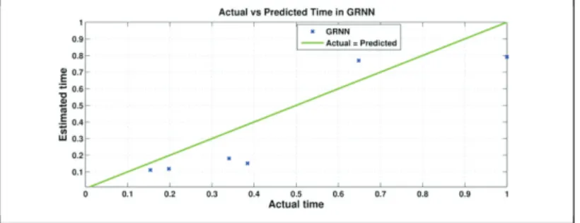
Fig. 2. Effort estimation model using GRNN
Figure 2 shows the deviation of predicted effort value from actual effort for General Regression Neural Networks. Nearer the points to the actual = predicted line in the figure, better is the prediction accuracy. In this study, the following values are used:
x Type of Kernel function: Reciprocal
x Minimum Sigma: 0.001
x Maximum Sigma: 0.5
x Model optimization and simplification Criteria: Minimize the error
The minimum and maximum values of sigma were chosen by taking the suitable combinations of values to generate best possible result. The values which gave the best results were chosen for testing. The network is trained using different sigma values (from 0.001 to 0.5) and the value of sigma which gives the best accuracy and least error is chosen as the final sigma value.
5.2 Model design using probabilistic neural networks
Probabilistic networks are mostly used for classification (Specht199018). For regression analysis i.e. employing PNN
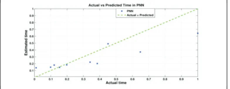
for prediction, first of all the number of classes in the dataset need to be found out. This can be done using any clustering mechanism. In this paper, k-means clustering technique is used. After finding out the number of classes and the inputs included under each class, some input vectors from each class are taken as example vectors and the dot product of example vectors and input vectors is found out. Then after applying the function mentioned above in section 3, the class node's activations were found out. The class node with highest activation was considered to be the predicted class for the current input and the numerical value (activation value) was used for performance evaluation. Figure 3 shows the deviation of predicted effort value from actual effort for PNN. The points nearer to the ideal prediction line shows more accurate prediction of effort. The lower prediction accuracy is reflected by the points scattered away from actual = predicted line.
It employs a supervised learning algorithm, which is bit different from back propagation algorithm. It has a feed forward architecture. There are no weights in its hidden layer. An example vector is associated with each hidden node, which acts as the weights to that hidden node. A PNN is comprised of an input layer, which is basically the input vector. This input layer is entirely connected with the hidden layer. Finally, an output layer depicts each of the conceivable classes for which the input data may be grouped. The hidden layer is not so much associated with this output layer. The example nodes for a specific class are joined with just that class's output node. For every class node, the sum of example vector (E) activations is figured out. Each hidden node's activation is the product of E and the input vector (F).
ܪൌ ܧכ ܨ (6) The class output activation is found out as:
ܥൌ σ ݁ఊమ ுିଵ ே
ୀଵ Τܰ (7)
where N is the number of example vectors for this class, Hi is the hidden node activation and gamma is the
smoothing parameter. The class, for which the input layer fits is dead set through a winner-takes-all methodology (i.e., the winning class is the output class node having the maximum class node activation).
Fig. 3. Effort estimation model using PNN
In this study, the following values are used:
x Type of Kernel function: Reciprocal
x Minimum Sigma: 0.001
x Maximum Sigma: 0.5
x Model optimization and simplification Criteria: Minimize the error.
The minimum and maximum values of sigma were chosen by taking the suitable combinations of values to generate best possible result. The values which gave the best results were chosen for testing. The network is trained using different sigma values (from 0.001 to 0.5) and the value of sigma which gives the best accuracy and least error is chosen as the final sigma value.
5.3 Model design using GMDH polynomial neural networks
GMDH networks date back to 1968 (first originated by Prof Alexey G. Ivakhnenko in Ivakhnenko11). They are
self-organizing networks i.e., the network's connections are not defined initially; instead, they are determined when the network is trained, with the objective of optimizing the network. Maximal accuracy is obtained by restricting the number of layers to be added to the network. This also helps prevent over-fitting. Initially a GMDH network starts with input layer only. This layer contains one unit for each input variable. The successive layer neurons derive their inputs from any two units of the previous layer. The final layer i.e., the output layer derives two of it's inputs from the previous layer and gives rise to one value (output of the network). Neurons in any layer can take input(s) from any of the previous layers. Two variable-quadratic polynomials are used as transfer functions in the neurons. These polynomials have the form:
ݕ ൌ ݔͲ ݔͳ כ ܽͳ ݔʹ כ ܽʹ ݔ͵ כ ܽͳଶ ݔͶ כ ܽʹଶ ݔͷ כ ܽͳ כ ܽʹ (8)
The training data is partitioned into two parts: training data and control data. Latter is used to halt the training process as soon as over-fitting starts. The algorithm adopted in this network works as follows: The transfer functions are used for defining all possible functions by combining inputs from the previous layer. Then, least
squares regression is applied for calculating ideal parameters for the transfer function in every neuron of the candidate list so that it best fits the training data. Then for every neuron, the MSE value is ascertained by employing it to the control data. Finally, the candidate neurons are arranged in ascending order of error and neurons with least error are picked up to be used in the next layer. In this work, following values are used for network parameters:
x Maximum no. of layers = 5
x Number of neurons per layer = 10 (fixed)
x Control data amount = 20\% of training data
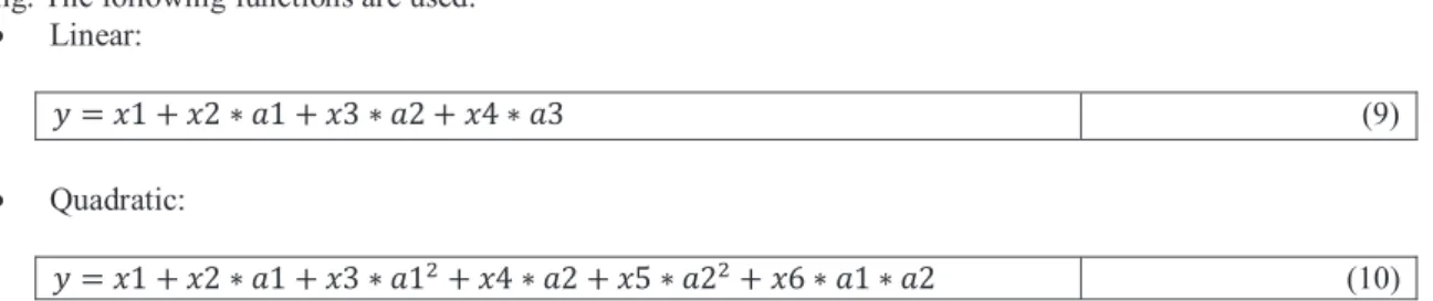
x Network layer connections: Connections from the former layer as well as the input layer are allowed. The parameters are self-explanatory. Values for parameters in this as well as the next model are fixed by taking the suitable combinations of values to generate best possible result, i.e. values which yield best results are chosen for testing. The following functions are used:
x Linear:
ݕ ൌ ݔͳ ݔʹ כ ܽͳ ݔ͵ כ ܽʹ ݔͶ כ ܽ͵ (9)
x Quadratic:
ݕ ൌ ݔͳ ݔʹ כ ܽͳ ݔ͵ כ ܽͳଶ ݔͶ כ ܽʹ ݔͷ כ ܽʹଶ ݔ כ ܽͳ כ ܽʹ (10)
Figure 4 shows the deviation of predicted effort value from actual effort for GMDH polynomial neural network. Nearer the points to the actual = predicted line in the figure, better is the prediction accuracy.
Fig. 4. Effort estimation model using GMDH Polynomial NN 5.4 Model design using Cascade Correlation neural networks
Cascade correlation neural networks (fahlman19) are also “self-organizing”. These networks initially have only an
input layer and an output layer. While training the network, neurons are chosen from a list of neurons and included in the hidden layer. The new neurons get their inputs from all the existing neurons of the network, hence it is called cascade. The training algorithm attempts to increase the amount of correlation between the newly added and the network's residual error (which has to be minimized). In this study, Gaussian kernel function is applied. The following network training parameters are used:
x Minimum neurons = 1
x Maximum neurons = 8
x Candidate Neurons = 8
x Maximum steps without improvement = 10
x Over-fitting protection control = 3-fold cross validation
Candidate neurons are the list of neurons from which hidden units are successively chosen and added to the network. Minimum number of neurons show how many hidden neurons must be added to the network. Maximum
number of neurons shows the maximum number of hidden neurons that can be added to the network. It is same as the number of candidate neurons, we can add one or more (even all) the candidate neurons to the network. The training process is continued till the results don't improve for a certain number of times, denoted by the maximum steps without improvement parameter. Cascade-correlation networks have this disadvantage of over-fitting the training data. Due to this, the accuracy values are quite high in case of training data, but low in testing data. So, for preventing this, the model is validated as it grows (3-fold cross validation is used). As stated earlier, the values which yield the best results are taken for testing.
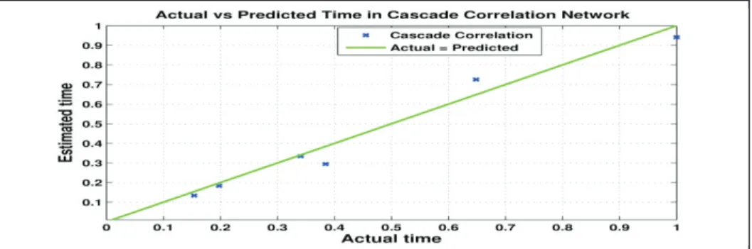
Figure 5 shows the deviation of predicted effort value from actual effort for cascade correlation neural network. Nearer the points to the actual = predicted line in the figure, better is the prediction accuracy.
Fig. 5. Effort estimation model using Cascade Correlation NN 6.Comparison
On comparing the results, it is observed that cascade correlation network performs better (gives better values of MSE, R2, MMRE and PRED) than other networks. Cascade correlation network is the best among the proposed
models and GRNN is the worst.
Table. 1. Comparison of our results with Existing work
Name of Technique Cascade Correlation NN General Regression NN Regression\cite{Zia}
PRED (%) 94.76 85.92 57.14
Table. 2. Comparison of Results obtained using three different types of neural networks
Name of metric MSE R2 MMRE PRED (%)
General Regression Neural Networks 0.0244 0.7125 0.3581 85.9182
Probabilistic Neural Networks 0.0276 0.6614 1.5776 87.6561
GMDH Polynomial Neural Network 0.0317 0.6259 0.1563 89.6689
Cascade Correlation Neural Network 0.0059 0.9303 0.1486 94.7649
Table 2 demonstrates the comparison of MSE, R$^2$, MMRE and PRED values for four different types of neural networks. Probabilistic neural network solves the optimization problem in an off line manner, hence it has low accuracy of prediction. GRNN also performs the prediction in an off line manner i.e. there is no real training of the network. The network parameters don't get optimal values, so the accuracy of prediction is lower than others. The self-organizing networks perform well because proper training is done for obtaining optimal network configuration with the objective of achieving maximum accuracy. Thus, the network built at the end of training best fits the data set and yields high values of accuracy when used on testing. Among the two self-organizing networks, Cascade-Correlation network performs better. The learning process in Cascade-Cascade-Correlation network is quick. The size and topology of the network are decided by the network itself. Moreover, error signals need not be back-propagated
through the network connections and the training is quite robust. The main advantage of GMDH networks is that they find weights using least squares fitting, which guarantees locally good weights. Back-propagation may be applied for obtaining globally-optimal weights. GMDH networks have this demerit of searching a polynomial network structure by only exploiting small neighborhoods. Alternative nodes are discarded when growing the network and not considered later in the learning process, which leaves chance for sub-optimal network structure, and hence the lesser prediction accuracy. But this particular problem doesn't exist in cascade-correlation networks.
7.Threats to validity
There are some areas which still remain un-addressed. This section aims to highlight those.
x All the effort estimation models proposed in this work have been developed by assuming that the initial project velocity value is given. This value is taken from the past projects developed by the same team in similar working conditions. But when a team is new, the company won't be having any past record for it. In that case, no clear assignment to initial project velocity can be done. However, the average velocity value of all the teams working in similar conditions can be taken and with nearly same size and assign it to initial project velocity and then proceed to use different neural network models to estimate the effort.
x In this study, data from Zia9 is used for implementation. It has records of twenty-one projects developed by six software houses. One shortcoming is there is no information about the type of projects taken for study. For our results to be valid for the general software engineering paradigm, the work should be based on data which covers all categories of software developed by agile methods. If it contains data of only one type of software, then the results of this work also apply to that particular type of software. Due to unavailability of details, this problem arises. However, since the data is about software developed by companies, it can be counted among the various effort estimation models developed so far.
x Due to small size of dataset, the testing data is very small in size. The data set size is 21 * 3, hence not much data is left for testing. Only six data points are used for testing. Thus optimal accuracy of the model's performance cannot be guaranteed.
8.Conclusion
The story point approach is one of the methods that can be used for developing mathematical models for agile software effort estimation. In this study, first the total number of story points and velocity of the project are considered in order to estimate the effort required during development of agile software. The resultant values are then optimized using various neural networks such as GRNN, PNN, GMDH networks and cascade networks. Toward the end of the study, the results obtained from various neural network models are empirically validated and compared in order to measure their performance. It is seen that cascade network outperformed other networks. The computations for above methodologies were executed, and results were obtained using MATLAB. Extension to this procedure might be made by implementing other machine learning techniques such as Stochastic Gradient Boosting (SGB), Random Forest etc. along with SPA.
References
1. Martin Fowler and Jim Highsmith. The agile manifesto. Software Development. San Francisco, CA: Miller Freeman, Inc; 2001. p. 28-35.
2. Shashank Mouli Satapathy and Aditi Panda and Santanu Kumar Rath. Story Point Approach based Agile Software Effort Estimation using Various SVR Kernel Methods. 2014 International Conference on Software Engineering \& Knowledge Engineering July 1-3, 2014 Hyatt Regency, Vancouver, Canada: 2014. p. 304-307.
3. Andreas Schmietendorf, Martin Kunz and Reiner Dumke. Effort estimation for Agile Software Development Projects. 5th Software Measurement European Forum: 2008. p. 113-123.
4. Pekka Abrahamsson, Outi Salo, Jussi Ronkainen, and Juhani Warsta. Agile software development methods: Review and analysis. VTT Finland: 2002.
5. David Cohen and Mikael Lindvall and Patricia Costa. An introduction to agile methods. Advances in Computers, Elsevier: 2003. p. 1-66.
6. Shashank Mouli Satapathy, Mukesh Kumar and Santanu Kumar Rath. Fuzzy-class point approach for software effort estimation using various adaptive regression methods. CSI Transactions on ICT, Springer: 2013. p. 367--380.
7. Siobhan Keaveney and Kieran Conboy. Cost estimation in agile development projects. ECIS: 2006. p. 183-197.
8. Evita Coelho and Anirban Basu. Effort Estimation in Agile Software Development using Story Points. Development: 2012.
9. Ziauddin Khan Zia, Shahid Kamal Tipu and Shahrukh Khan Zia. An Effort Estimation Model for Agile Software Development. Advances in Computer Science and its Applications: 2012. p. 314-324.
10. Scott E Fahlman and Christian Lebiere. The cascade-correlation learning architecture. 1989.
11. AG Ivakhnenko. Heuristic self-organization in problems of engineering cybernetics. Automatica, Elsevier: 1970. p. 207-219.
12. Shashank Mouli Satapathy, Barada Prasanna Acharya and Santanu Kumar Rath. Class Point Approach for Software Effort Estimation Using Stochastic Gradient Boosting Technique. ACM SIGSOFT Softw. Eng. Notes,ACM : 2014. p. 1-6.
13. Tim Menzies and Zhihao Chen, Jairus Hihn and Karen Lum. Selecting best practices for effort estimation. Software Engineering, IEEE Transactions, IEEE: 2006. p. 883-895.
14. Rashmi Popli and Naresh Chauhan. Cost and effort estimation in agile software development. Optimization, Reliabilty, and Information Technology (ICROIT), 2014 International Conference, IEEE: 2014. p. 57-61.
15. Ishrar Hussain, Leila Kosseim and Olga Ormandjieva. Approximation of COSMIC functional size to support early effort estimation in Agile. Data & Knowledge Engineering, Elsevier: 2013. p. 2-14.
16. Alaa El Deen Hamouda. Using Agile Story Points as an Estimation Technique in CMMI Organizations. Agile Conference (AGILE), IEEE: 2014. p. 16-23.
17. Donald F Specht. A general regression neural network. Neural Networks, IEEE Transactions, IEEE: 1991. p. 568-576.
18. Donald F Specht. Probabilistic neural networks. Neural networks, Elsevier: 1990. p. 109-118.
19. Scott Fahlman Christian and Christian Lebiere. The Cascade-Correlation Learning Architecture. Advances in Neural Information Processing Systems. 1990.
20. Stanley J Farlow. Self-organizing methods in modeling: GMDH type algorithms. CrC Press: 1984.
21. PVGD Reddy, KR Sudha, P Rama Sree and SNSVSC Ramesh. Software effort estimation using radial basis and generalized regression neural networks. 2010.
22. Parasana Sankara Rao and Reddi Kiran Kumar. Software Effort Estimation through a Generalized Regression Neural Network. Emerging ICT for Bridging the Future-Proceedings of the 49th Annual Convention of the Computer Society of India (CSI) Volume 1, Springer: 2015. p. 19-30.
23. Rashmi Popli and Naresh Chauhan. Estimation in agile environment using resistance factors. Information Systems and Computer Networks (ISCON), 2014 International Conference, IEEE: 2014. p. 60-65.
24. Parag C Pendharkar. Probabilistic estimation of software size and effort. Expert Systems with Applications, Elsevier: 2010. p. 4435--4440.