THE GEOMETRY OF DOUBLE AFFINE HECKE ALGEBRA SUPERPOLYNOMIALS
Ian Philipp
A dissertation submitted to the faculty at the University of North Carolina at Chapel Hill in partial fulfillment of the requirements for the degree of Doctor of Philosophy in the Department of Mathematics in
the College of Arts and Sciences.
Chapel Hill 2018
Approved by:
Ivan Cherednik
Prakash Belkale
Jiuzu Hong
Lev Rozansky
c
2018 Ian Philipp
ABSTRACT
Ian Philipp:
The Geometry of Double Affine Hecke Algebra
Superpolynomials
(Under the direction of Ivan Cherednik)
We formulate a conjecture which interprets DAHA superpolynomials colored by fundamental weights to
the Borel-Moore cohomology of Jacobian factors and their flagged and higher rank generalizations. To study
the generalized Jacobian factors we use a certain stratification derived from the valuation semi-group of the
singularity and in special cases show that the components of the stratification of the flagged Jacobian factors
and higher rank Jacobian factors are affine spaces. Once these results are in place it is easy to check the main
conjecture. In the last section, we are able to check the conjecture for more sophisticated examples where the
stratification does not consist of affine cells and study for a particular example which types of varieties may
TABLE OF CONTENTS
LIST OF TABLES . . . vii
CHAPTER 1:
INTRODUCTION
. . . 1CHAPTER 2:
BACKGROUND
. . . 32.1
DAHA superpolynomials
. . . 32.1.1
DAHA of type
GLn . . . 32.1.2
DAHA-Jones theory
. . . 62.2
Jacobian factors
. . . 8CHAPTER 3:
MAIN CONJECTURE
. . . 123.1
Spaces of Flags
. . . 123.2
Spaces of Higher Rank Modules
. . . 133.3
Main Conjecture
. . . 23CHAPTER 4:
A FAMILY OF ITERATED TORUS KNOTS
. . . 274.1
Dimensions of Spaces of Rank 1 Flags
. . . 274.2
Basic Definitions
. . . 284.3
The cells for flagged Jacobian factors are affine
. . . 294.4
Calculating dimensions
. . . 31CHAPTER 5:
HIGHER RANK MODULES AND TORUS KNOTS
. . . 345.1
Main claims
. . . 345.1.1 Basic definitions . . . 34
5.1.2 Theorems 5.1.1,5.1.2 . . . 35
5.1.3 Reduction algorithm. . . 36
5.2
Proof of Theorem 5.1.1
. . . 365.2.1 Syzygies ofk[Γ]-modules . . . 36
5.2.2 Jrk(∆)is affine . . . 38
5.3.1 Computingµ∆,g . . . 40
CHAPTER 6:
NUMERICAL SIMULATIONS
. . . 436.1
Uncolored Computations
. . . 436.1.1 Two simplest cables . . . 44
6.2
Colored by Columns
. . . 466.2.1
Numerical simulations
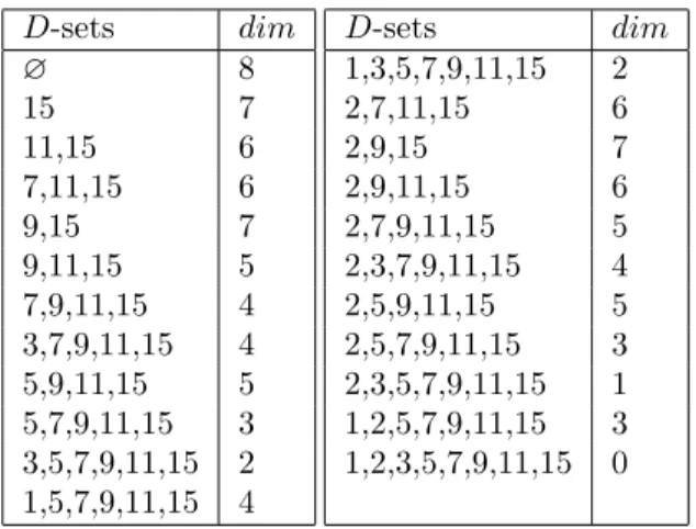
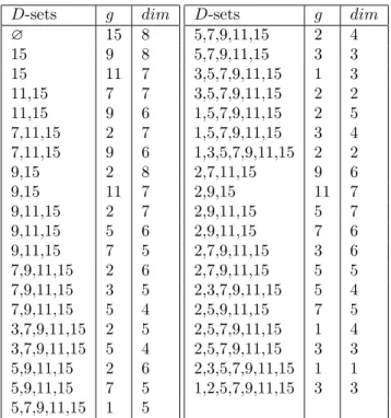
. . . 466.2.2 Non-affine cells forv= 9,15 . . . 50
6.2.3 R=C[[z4, z6+z7]], `= 0The case v=7, length=0 . . . 53
LIST OF TABLES
6.1 Dimensions for Γ =h4,6,13i, m= 0 . . . 44
6.2 Dimensions for Γ =h4,6,13i, m= 1 . . . 45
6.3 Dimensions for Γ =h4,6,13i, m= 2 . . . 45
6.4
Types of cells for
R=C[[z4, z6+z9]]when
`= 0,1:
. . . . 506.5 Non-affine types forrk= 2, Γ =h4,6,6 +vi . . . 52
6.6
Types of cells for
R=C[[z4, z6+z15]]when
`= 0:
. . . 52CHAPTER 1
Introduction
Given a plane curve singularity C at the origin inC2, one may associate a linkL toC by intersecting
the boundary ofS3 with sufficiently small radius with C and we call such linksalgebraic links. It is then
interesting to study whether invariants ofL have an algebraic geometric interpretation. For example, the
intersection multiplicity of the branches ofC is equal to the linking number of L and also the Alexander
polynomial ofL is given by the semi-group of the singularity.
In [Ch2], Cherednik used double affine Hecke algebras (DAHA) to introduce deformations of the Jones
polynomial of torus knots and present some conjectures concerning their stabilizations known as DAHA
superpolynomials. Building upon this work, in [ChD1] this definition was expanded to iterated torus knots
and in particular all algebraic knots.
In this thesis we continue this tradition by giving a conjecture which interprets DAHA superpolynomials,
new invariants of knots conjecturally related to Khovanov-Rozansky homology, to the Borel-Moore cohomology
of Jacobian factors and their new generalizations. Jacobian factors are local versions of the compactified
jacobian of singular curves. Instead of locally free rank 1 sheaves on the curve, we consider the moduli space
of modules over the complete local ring ofC.
Let us briefly summarize each chapter below: Chapter 2 introduces the definition of DAHA
superpolyno-mials for algebraic knots and the relevant basics on Jacobian factors. Note that our study focuses only on
DAHA of typeGLn although DAHA superpolynomials themselves are defined for all colors and root systems.
However, the geometry for types besidesGLn remains mysterious.
In chapter 3, we introduce the main new objects in this work, the flagged Jacobian factors and their
higher rank counter parts. The main conjecture states that the Borel-Moore cohomology of these objects
categorifies the DAHA superpolynomial in a certain sense.
In chapter 4, we prove that for the family of singularitiesk[[z4, z2u+zv]] withv >2u,v odd, the rank 1
flagged Jacobian factors are affine spaces and we calculate their dimensions in terms of the semi-group of the
singularity.
In chapter 5, we show that for all torus knots the flagged Jacobian factors in all ranks are affine spaces
Finally, in chapter 6 we supply a large number of calculations that provide ample evidence for the main
conjecture. Very important here are cases when the stratification used in chapters 4 and 5 do not supply a
CHAPTER 2
Background
2.1
DAHA superpolynomials
In this section we will briefly summarize the necessary theory for the reader to understand the definition
of DAHA superpolynomials forGLn. Note that DAHA-Jones polynomials are well defined for all simple root
systems and weights (see [ChD1]). The theory of DAHA superpolynomials, however exists only in typeA
although there are some developments (mostly conjectures) for classical root systems and even a couple of
examples in typeE; see [Ch2, ChP].
2.1.1
DAHA of type
GLnLet us begin with the definition of DAHA itself. See [Ch1] for details.
Definition 2.1.1. The double affine Hecke algebra HH(referred to as DAHA) of GLn is an algebra over
Cq,t ==defC(q1/2, t1/2)generated by Ti±1, X ±1
j and π, where1≤i≤n−1, 1≤j≤n, which are subject to the
following relations:
(i) (Ti−t1/2)(Ti+t−1/2) = 0, TiTi+1Ti =Ti+1TiTi+1,
(ii) TiTk =TkTi if |i−k|>1,
(iii) XjXk=XkXj (1≤j, k≤n), TiXiTi =Xi+1 (i < n),
(iv) πXi =Xi+1π(1≤i≤n−1) and πnXi=q−1Xiπn (1≤i≤n),
(v) πTi=Ti+1π (1≤i≤n−2) and πnTi =Tiπn (1≤i≤n−1).
The subalgebra ofHHgenerated byTi for 1≤i≤n−1iis isomorphic to the (non-affine) Hecke algebra
of typeGLn. The followingself-duality is the key in DAHA theory. Let us define pairwise commutativeYi
(1≤i≤n) inductively as follows:
to the extended affine Hecke algebra of typeGLnand the aforementioned duality is given by an anti-involution ofHH, sending
ϕ:Xj ↔Yj−1(1≤j≤n), Ti7→Ti(1≤i < n) and fixing q1/2, t1/2.
Braid group action onHH. Along withϕ, the symmetries ofHHinclude an action of the braid groupB3 on
three strands. Its two generators act as follows:
τ+(Xi) =Xi, τ+(Y1· · ·Yi) =q−i/2(X1· · ·Xi)(Y1· · ·Yi), (2.1)
τ−(Yi) =Yi, τ−(X1· · ·Xi) = qi/2(Y1· · ·Yi) (X1· · ·Xi),
where τ+, τ− fixTi and q1/2, t1/2. They satisfy τ+τ−−1τ+ =τ−−1τ+τ−−1, the defining relations of B3. This
group is naturally a central extension ofP SL2(Z); the covering map is
τ+7→
1 1
0 1
, τ−7→
1 0
1 1
. (2.2)
See [Ch1], Section 3.7 for details. We note thatτ+ is the conjugation ofYi by theGaussian γ=qPni=1x 2 i/2,
where we put formallyXi =qxi.
Polynomial representation We will use the standard basis{j,1≤j ≤n} inRn, supplied with the inner
product (i, j) =δij. Letαi=i−i−1 be simple roots forgln, {α=i−j, i < j}the set of positive roots, ρ= (1/2)P
α>0α, W=S
n the symmetric group,si = (i, i+ 1) simple reflections. The fundamental roots
areωi=1+2+...+i. Note that (ρ, i) = (n−(2i−1))/2, (ρ, ωi) =i(n−i)/2, (ρ, i−j) =j−i. The
latticesQ, P are correspondingly formed by integer linear combinations of{α},{ωi}. Dominant weights are b=Pb
iωi bi∈Z+; we use the notation isb∈P+.
Affine Weyl group. LetRe={[α, j], α∈R, j∈Z} be the affine root system of typeA. Affine positive roots
are forj >0 or withα >0 ifj= 0. Theextended Weyl group Wc is the semidirect productW
n
P, wherethe action inCn+13[z, ζ] is:
(wb)([z, ζ]) = [w(z), ζ−(z, b)] for w∈W, b∈P. (2.3)
It containsfW
def
==hsi,0≤i≤n−1iwhereα0= [1,−θ], and where θ=1−n is the maximal positive root.
c
W is naturally isomorphic toWf
o
Π for Πdef
==P/Q. Setting wb=πm
e
w∈Wcfor m∈Z,we∈fW, the length
is the subgroup ofcW of the elements of length 0. Coinvariant. For wb = πm
e
w ∈ Wc and a reduced decomposition we = si`· · ·si1 of length ` = `(wb), we set
T
b
w=πmTi`· · ·Ti1. There is a unique presentation of anyH ∈ HHas a sum of (
Q
Xjuj)Tw(Q
Yjvj), where
uj, vj∈Z, w∈W; this is a DAHA counterpart of the PBW Theorem. We use this to define thecoinvariant
{·}ev:HH →Cq,t, {Xj}ev=t−(ρ,j),{Yj}ev=t(ρ,k),{Ti}ev=t1/2. (2.4)
By construction: {ϕ(H)}ev={H}ev forH ∈ HH.
The coinvariant factors through the polynomial representation X of HH. Let χ be the following
one-dimensional character of the affine Hecke algebra HY: χ(Ti) = {Ti}ev = t1/2, χ(Yj) = {Yj}ev. Then
X def
== IndHHYH(χ). We will use the following projection ofHHontoX:
HH 3H7→H⇓def== Hb(1)∈X, (2.5)
whereHb is the image ofH in End(X). Thecoinvariant is then{H}ev={H⇓}ev, where the latter evaluation
sendsXj 7→ {Xj}ev.
Macdonald Polynomials The polynomial representation is given explicitly by theDemazure-Lusztig operators:
Ti = t1/2si + (t1/2−t−1/2)(Xαi−1)−1(si−1), 0≤i≤n. (2.6)
The elementsXbbecome the multiplication operators inX;πm∈Π act via the general formulawb(Xb) =Xw(b)b
forwb∈Wc, whereX[b,j] def
==qjX
b. The starting point of the DAHA theory was addingT0here forα0= [1,−θ],
where θ=1−n is the maximal positive root.
The E andP polynomials. The nonsymmetric Macdonald polynomials Eb for b∈P are eigenvectors of cYj
(the images of Yj in End(X)). This definition fixes them uniquely up to proportionality for genericq, t; the
normalization is to make the coefficient of Xb equal to 1. Thesymmetric Macdonald polynomials Pb are
defined fordominant b=Pb
iωi,bi∈Z+. In terms ofEb, one has: Pb=PEb, where
Pdef== X
w∈W
t`(w)−1 X
w∈W
t`(w)/2Tw is thet-symmetrizer.
See [Ch1], (3.3.14). The coefficient ofXb is 1 inPb as well.
The following evaluation formula (the Macdonald Evaluation Conjecture) is important for DAHA
super-polynomials:
Pb(t−ρ) =t−(ρ,b)Y α>0
(α,b)−1
Y
j=0
1−qjtXα(tρ)
1−qjX α(tρ)
, (2.7)
where X[b,j](tc) def
==qjt(b,c). The evaluation can be herePb(t±ρ), but the corresponding evaluation formulas
forEb must be exactly att−ρ; see (3.3.16) from [Ch1].
2.1.2
DAHA-Jones theory
Algebraic knotsIn this section, we briefly review the necessary aspects of algebraic knots. See e.g. [EN]
for details.
Let Cbe the germ of a unibranch plane curve singularity at 0∈C2. The intersection ofCwith a smallS3
centered at 0 is the correspondingalgebraic knot LC, called the link ofC. We will use the notationLwhen
there is no ambiguity. All algebraic knots areiterated torus knots, but generally iterated torus knots are not
algebraic.
The Newton-Puiseux presentation ofC is as follows:
y=x s1 r1(c1+x
s2
r1r2 c2+. . .+x sl
r1r2···rl) centered at 0. (2.8)
The pairs {ri,si} are known as Newton pairs. They are positive integers such that gcd(r,s) = 1. The
parameterscj here are assumed sufficiently general.
The torus knot T(r,s) is for one pair{r,s}. Topologically, it lies on the surface of a torus and wrapsr
times around the torus longitudinally andstimes around latitudinally. Due to the isotopyT(r,s) =T(s,r), we may assumer>s. For anyl, let
~r={r1, . . .rl}, ~s={s1, . . .sl}, (2.9)
a1=s1,ai=ai−1ri−1ri+si (i= 2, . . . , l).
The pairs {aj,rj}are topological invariants ofLC, the Newton pairs are not.
The knot LC can be described topologically as follows:
Hereis the unknot andCabis thecabling procedure defined as follows. For any oriented knotK embedded
in the 3-sphere consider a small torus aroundK which does not intersect itself. ThenCab(a,b)(K) is the knot created by placingT(a,b) on this torus. We omit details, but let us remark that we can assume now thatr1>s1 only for the first pair of indices.
Main construction Now we will review DAHA-Jones polynomials and DAHA superpolynomials. The main
source for this content is [ChD1].
Generally, for any polynomialF in fractional powers ofqandt, itstilde-normalizationFeis the result ofF
divided by the lowestq, t-monomial, assuming it is well defined. We will use the notationq•t•for a monomial
factor (possibly with fractional exponents) in terms of q, t. We will also use the tilde-normalization for
superpolynomials, where the lowestq, t-monomial is chosen from the those terms without the third parameter
a(i.e. ata= 0).
The following theorem is from [ChD1] and is stated there for arbitrary root systems. Recall (2.4) and
(2.5), the definitions of the coinvariant and the projection ontoX.
Theorem 2.1.2. (i) Given two strictly positive sequences~r,~sof lengthl as in (2.9), letγi∈P SL2(Z)be the
element whose representative is the matrix with first column(ri,si)tr (tr indicates transpose). Let γib be a lift
ofγi to theB3 via the homomorphism (2.2). For a dominant weight bofGLn, theDAHA-Jones polynomial is
JDGLn
~r,~s (b; q, t) = JD~r,~s(b;q, t) def
== (2.11)
n
b
γ1· · ·γl−1b bγl(Pb)/Pb(t−ρ)
⇓⇓· · ·o ev
.
It does not depend on the particular choice of the lifts γi and bγi. Thetilde-normalizationJDf~r,~s(b;q, t)is well
defined and is a polynomial in terms of q, twith the constant term 1. (ii) Now consider a given dominant b=Pn
i=1biωi from (i) as a (dominant) weight for anyglm provided
m≥n−1. We make the convention thatωn = 0upon the restriction togln−1.
Given sequences~r,~sas above, there exists a DAHA superpolynomial H~r,~s(b;q, t, a)belonging toZ[q, t, a]
satisfying the relations
H~r,~s(b;q, t, a=−tm+1) =JDf
GLm
~r,~s (b;q, t) for anym≥n−1; (2.12)
its a−constant term is automatically tilde-normalized. The formula 2.12 uniquely determines H~r,~s. This
It is important (theoretically and practically) that one may use non-symmetricEbin place of the symmetric
Pb; this results in the same super-polynomial. TheE polynomials do not occur in classical Lie theory; so
usingE polynomials is an advantage for the theory of DAHA superpolynomials, and a clear challenge for
other approaches. Computationally, the programs written in terms ofEpolynomials are much faster.
Khovanov-Rozansky homology Concerning the topological invariance of H~r,~s(b;q, t, a), it is expected from
[ChD1] thatH~r,~s coincides with thereduced stable Khovanov-Rozansky polynomial of the corresponding knot;
see [KhR1], [KhR2], [Kh]. To be precise, it is conjectured that
H~r,~s(ω1;q, t, a)st=KhRstabg (qst, tst, ast). (2.13)
The subscriptstindicates that we have made the substitution to thestandard topological parametersgiven by
t=qst2, q= (qsttst)2, a=a2sttst, qst2 =t, tst=
p
q/t, a2st=a
p
t/q. (2.14)
g
KhRstabis thereduced KhRstab polynomial divided by the smallest power ofast and then byqst•t•st such that
g
KhRstab(ast= 0)∈Z+[qst, tst] and the constant term of this polynomial equals 1.
The stable KhR-polynomials are sufficiently understood only in the uncolored case, so the DAHA
construction must be restricted tob=ω1here. The minuscule weights may be managed in thecategorification theory, though explicit formulas (to compare with our ones) are still not available. The reduced setting is
also a problem. Generally, formulas for KhR polynomials are quite a challenge; for uncoloredtorus knots,
there is recent progress based on Soergel modules [Mel].
2.2
Jacobian factors
Jacobian factors are local analogues of the compactified Jacobians of singular curves. In this section we
provide the necessary background in jacobian factors following [GP].
Rank one torsion-free modules Letkbe any field;k its algebraic closure,O=k[[z]],K=k((z)),Rbe any
k−subalgebra ofOcontaining some principle ideal (zm) =zmO ⊂ O. We willnot assume for now thatRis
a ring of a plane curve singularity, which is by definition an algebra with two generators overk(this is due to the Newton-Puiseux theorem mentioned above).
δ−invariant (the arithmetic genus) of R is thenδ =δR def
== dimC(O/R) =|Z+\ΓR|, where | · | is the
cardinality. We will call Z+\ΓR theset of gaps and denote itGR. Letc=cR be theconductor ofR, the
smallest integer such that (zc) =zcO ⊂ R. One has, c≤2δ, where the equality holds exactly for Gorenstein
R(including plane curve singularities and this result is due to Gorenstein himself); this equality is equivalent toδ=|ΓR\(c+Z+)|.
Standard modules For any nonzeroR−submodule M ⊂ O, its O−degree, the degree with respect toO is degO(M)==dimdef k(O/M). One has degOR=δ. For arbitrary submodulesM ⊂ K, we set:
degO(M)== dimdef C(O/(O ∩M))−dimC(M/(O ∩M)). (2.15)
Thedeviation ofM overRis
dev(M)==def−degR(M) =δ−degO(M). (2.16)
Let ∆M = ∆(M)
def
== ν(M); it is a Γ−module, i.e. by definition Γ + ∆ ⊂∆. The conductor cM of M is
naturally the smallestc∈Z+such that zcO ⊂M. Equivalently, it is the smallestcsuch that ∆
M ⊃c+Z+.
We call ∆M standard if Γ⊂∆M, i.e. M contains somex∈1+zO. For standardM: degO(M) =|Z+\∆M|, dev(M) =|∆M\Γ|. We will use the notations degO(∆) anddev(∆) for the right-hand sides here when ∆ = ∆M
and for any standard Γ-module ∆ (not necessarily the set of valuations of a module overR).
Invertible modules are standard ones with one generator (thus the generator must be an element of
1 +zO). Accordingly, 1) ∆M = Γ, 2)dev(M) = 0 and 3)cM =cfor invertibleM; vice versa, any standard M satisfying one of these three conditions is invertible. The latter implication is obvious for the first two equalities and the invertibility follows fromcM =cdue to the following general lemma.
Lemma 2.2.1. For any standardR−module M,cM ≤c−dev(M).
Proof. We follow [PS], but need a bit different form of their condition (ii) from Section 1. Also, we provide the proof since this lemma is an important particular step of the generalization (below) to arbitrary
ranks. SincecM −1 is missing in ∆M (so missing in Γ too), all cM−1−γ for anyγ∈Γ are not in ∆M, and
one has:
δ−dev(M) = |Z+\∆M| ≥ |{γ∈Γ | ν(γ)<cM}|
Any module M can be canonically transformed to a standard one M◦ as follows: M◦ = z−nM for n =min ∆M. Indeed, degO(znM) = degO(M) +n and dev(znM) = dev(M)−n for any M, n. We set
∆◦M = ∆(M◦) = ∆−nand writedev◦(M) =dev(M◦),c◦M =cM◦.
Using the mapπ:M =M◦7→zdev(M)M, the space of standardR−modules can be identified with the
set of allR−modules of degreeδ=δR (equivalently, of deviation 0). The latter modules have conductors at
leastc(and therefore at least 2δ). Indeed,cπ(M)=c◦M+dev(M)≤cdue to the lemma. Respectively, we set π(∆)== ∆ +def dev(∆) for any standard ∆.
This observation readily identifies the space of standard modules considered under πwith theprojective
variety ofall R−invariant subspaces of co-dimensionδin O/zcO, calledMin [PS]. They actually consider O/z2δO, but this results in the same variety. Recall thatc= 2δ for GorensteinR.
We will denote this projective variety byπJ
Rand identify it when necessary with the space of all standard
modules denoted byJ =JR.
For standard ∆, let
J(∆)==def{M =M◦ | ∆(M) = ∆}; also we represent: (2.17)
π(∆) = ∆ +dev(∆) ={d1< d2< . . . < dδ} ∪ {2δ+Z+}. (2.18)
Using the theory of Schubert varieties and following [PS],
Closure (πJ(∆))⊂S
∆0 πJ(∆0) for ∆0 such that d0i≥di, (2.19)
where 1≤i≤δ.
By the closed fiber of an R−module M, we mean M = M/mM for the maximal ideal m ⊂ R. Its
dimension overkwill be called theNakayama rank. The Γ−rank of ∆ = ∆M is the number of generators bi
of ∆ over Γ. These generators are exactly all primitive (indecomposable) elements, i.e. those not in the form
a+γ fora∈∆ and 0< γ∈Γ. Equivalently, they can be introduced by the following conditions: ∆\ {bi}
are Γ−modules. The Γ−rank of ∆ is no greater than$ == mindef {γ >0 | γ ∈Γ}, themultiplicity of the singularity associated withR.
Lemma 2.2.2. The Nakayama rankdimkM of any M is no greater than theΓ−rank of∆M, and no greater
than$. If the primitive elements of ∆ = ∆M are all smaller than the first non-primitive element in∆, then
Proof. The images of the elementsmi ∈M such thatν(mi) are primitive generateM. If the primitive elements of ∆M are all smaller than the first non-primitive element in ∆ then the images of themi will form
a basis forM.
Example 2.2.3. The simplest example of a moduleM with maximal possible Nakayama rank $ isM=O. Then∆M =Z+,{0,1, . . . , $−1} are primitive elements. For any0≤i < $, one can diminish this module
M =O as follows. LetOhii= ⊕i−1j=0ke0j
⊕zi+1Ofor e0
j =zj+λjzi, where λj ∈k(0≤j≤i−1)are any
(free) parameters. Then ∆(Ohii) =Z+\{i} and the primitive elements are {0,1, . . . , $−1} \ {i}; so the
Nakayama rank of Ohiiis$−1 and it depends oni (free) parameters.
Admissibility. A Γ−module ∆ is calledadmissible if there existsM such that ∆M = ∆. All Γ−modules are
admissible formonomial R(quasi-homogeneous singularities); see [PS]. MonomialRarek−subalgebras in
Ogenerated by pure monomialsza. This is a significant simplification of the general theory of ∆ andM;
CHAPTER 3
Main Conjecture
In order to state the main conjecture we need to define certain spaces of flags of modules over the
curve singularity. We start by providing the definition for rank 1 modules and then we will generalize this
construction to higher rank modules.
3.1
Spaces of Flags
Standard flags These were first defined in [ChP]. A flag−M→={M0 ⊂M1 ⊂. . . ⊂M`} of R−modules
Mi ⊂ Oas above is calledfullν−increasing if the corresponding ∆−flag−→∆ = ∆(M−→) ={∆0⊂∆1⊂. . .⊂∆`}
for ∆i= ∆(Mi) is full increasing, i.e. satisfies the following:
∆i = ∆i−1∪ {gi}, g1< g2< . . . < g`, 1≤i≤`. (3.1)
It is called standard if it is fullν−increasing and M0 is standard (i.e. ∆0 ⊃Γ), which automatically
implies that allMi are standard. We will call such (standard) flags simply`−flags and define the length of
−→
M byl(−M→) =`.
The setJ` of all standard`−flags−M→is called theflagged Jacobian factor in [ChP]. It can be supplied with a natural structure ofquasi-projective variety. This requires the following proposition, which is actually
Proposition 2.3 from [ChP] (somewhat related to [ORS], Section 2.1). Its proof there did not use thatRis of planar (with 2 generators), so we will omit it.
For an arbitrary module M, we setM{i}=M ∩(zi), which is obviously anR−module,M{i}the image
ofM{i} in M. One has: dimM{g}/M{g+1}= 1 for g∈∆M and 0 otherwise. These dimensions can drop to 0
upon taking the closed fiber, which is the reduction modulom.
Proposition 3.1.1. (i) For a full increasing ∆−flag −→∆ =
∆0⊂ ∆1= ∆0∪ {g1} ⊂ · · · ⊂ ∆`= ∆0∪ {g1, . . . , g`} , all∆0∪ {gi} for1≤i≤`are Γ−modules. This implies that for any standard flag
−→
M of length
`, one has: mM`⊂Mi for 0≤i≤`. The Mi are uniquely determined by their imagesM0i ==defMi/mM` in
M`, which follows from Nakayama’s Lemma.
of Nakayama rank. Given−→∆ andM`, all possible M0 are in one-to-one correspondence with k−subspaces M006⊂M{1}` of codimension `such that
dimk(M 0 0+M
{gi} ` )/(M
0 0+M
{gi+1}
` ) = 1 for 1≤i≤`. (3.2)
(iii) Given−→∆ and a standardM`, the corresponding`−flags −M→exist if and only if
dimkM{g` i}/M {gi+1}
` = 1 for 1≤i≤`. (3.3)
These flags can be identified via Nakayama’s Lemma with full`−flags ofk−subspaces M00⊂. . .⊂M0i⊂. . .⊂ M` such that
M0i+M{gi+1}` =M` for 1≤i≤`−1. (3.4)
Provided (3.3) and givenM0, this space is biregular to A`(`−1)/2.
Example 2.2.3 can be interpreted as follows. All 1-flags (for`= 1) withM1=O are{M0=Ohii ⊂ O=
M1}. Giveni, the corresponding subspaces ofO/z$O ∼=k$ of codimension 1 must contain (zi+1) but not
(zi). Thus the space of such flags is biregular toAi, which matches Example 2.2.3. Herei≥1; note that the
removal ofi= 0 fromZ+makes the corresponding module non-standard.
Proposition 3.1.1 identifiesJ` with the space of pairs
M`∈Jh`i,{M 0
i,0≤i≤`} ,
where (a) Jh`i ⊂J is a projective subvarietyπJ of modules of Nakayama rank no smaller than`considered
under the map πabove, (b) M00⊂M` is ak−subspace of codimension `such that M06⊂M
{1}
` , and (c)
{M0}isany full flag inM`/M00. Following the notation forrk= 1 above, we will denote this variety byπJ`
or simply byJ`.
3.2
Spaces of Higher Rank Modules
Let us consider now R−submodulesM ⊂ Ork ofrk≥1 such thatK · M=Krk. From now on, we fix an
Basic definitions As in the case ofrk= 1, theO−degree ofM ⊂ Orkis naturally deg O(M)
def
==dimk(Ork/M);
for arbitrary submodulesM ⊂ Krk of rankrk overK, we set:
degO(M)== dimdef k(Ork/(Ork∩ M))−dimk(M/(Ork∩ M)). (3.5)
Thedeviation ofMfromRrk isdev(M)==def rk·δ−deg O(M).
Theprojections ofMontoi, their Γ−modules and the corresponding deviations are:
Mhii == (def M, i),∆hii= ∆hii(M) = ∆(Mhii),
devhii(M) =dev(∆hii) for 0≤i≤rk−1. (3.6)
These definitions significantly depend on the choice of the basis{i}.
∆−Components. There is another way to associate a sequence of Γ−modules toM; it will be the main tool for us. It requires a choice ofcumulative valuation υ:Krk→
R, extending the valuationν above:
υ(X
i
mii) = min
i {ν(mi)+υ(i)} for mi∈ K, 0≤i≤rk−1, (3.7)
where υi ==def υ(i) can generally be arbitrary real numbers. The conditions 0≤υi 6=υj <1 for i6=j are sufficient below and will be imposed unless stated otherwise. Generally, one needs the following weaker
relationsυi−υj 6∈Zfori6=j. A convenient choice will beυi=i/rk.
For suchυand 0≤i≤rk−1, the ∆−components are Γ−modules defined as follows. Let ∆(M)==defυ(M) so that we may define,
∆(i)(M) ={a∈Z+|a+υi∈∆(M)}, dev(i)=dev(∆(i)(M)). (3.8)
We will also use the notation ∆(i)M = ∆(i)(M) or simply ∆(i) when there is no fear of confusion. It is
immediate to check that ∆(i)⊂∆hii.
Our definition of Piontkowski-type cells will be based on{∆(i)}; the modules{∆hii}are needed to define
the map stbelow. Importantly,Prk−1
i=0 dev
(i)=dev(M), as well as the analogous formula Prk−1
i=0 deg (i)
=
degO(M), where deg(i)= deg ∆(i)=|
Z+\∆(i)|and degO(M). These relations generally do not hold for ∆hii.
It is interesting to examine the dependence of{∆(i)}upon the change of basis{i} 7→ {bi}without varying the numbersυi.
M ⊂ Ork be an R-module such thatK · M = Krk. Define an upper-triangular linear substitution on M
as follows: i 7→ bi=i+ P
j<ic j
ij, where c j
i ∈ k (apart from some finite set of affine hyperplanes). If
c
M==def{Prk−1
i=0(y, i)bi | y∈ M}, thenν(Mc)has the following components:
b
∆(0)= ∆(0)∪. . .∪∆(rk−1), ∆b(1)=Si6=j{∆(i)∩∆(j)}, . . . ,
b
∆(rk−2)=S
i
∩j6=i∆(j) , ∆b
(rk−1)
= ∆(0)∩. . .∩∆(rk−1).
If kis infinite, kis not needed here: cji ∈k. Also, lower-triangular substitutions i7→bi=i+ P
j>ic j ij, do
not influence ∆(i).
Proof. The case of upper-triangular transformations involving two neighboring i, i+1 is sufficient
to consider for both claims. Suppose y = tm
i +ctmi+1 +tmPj>i+1ajj mod (tm+1)O2, and y0 = tn
i+1+tnPj>i+1bjj mod (tn+1)O2 wherec, aj, bj are constants. The corresponding valuations are then m+υi andn+υi+1. It suffices to consider elements only in the form ofyand y0.
Obviously lower-triangular substitutions will not change the valuationsy andy0. Let us justify the first claim. Giveny, let’s first assume that elements of the form ofy0 appear only forn6=m. Then a single change
i+17→i+1+αi forα∈k∗ will preserve the valuation of yifα+c6= 0 and will change the valuation ofy0
ton+υi. Thusnwill be added to ∆(i) and will disappear from ∆(i+1) in this case.
Note that ifα+c= 0 here, thenm∈∆(i)andn∈∆(i+1)will be transposed, so a different transformation
will occur. Therefore for k =F2, moving n from ∆(i) to ∆(i+1) is not possible over k ifc = 1 and more
general substitutions (not only upper-triangular) must be considered or, as in the lemma, one may usek.
Now giveny, supposey0 exists withn=m, which means that m∈∆(i)∩∆(i+1). Then mremains in
both, ∆(i)and ∆(i+1), upon the substitution above for anyα.
We see that the resulting components forα+c6= 0 become ∆(i)∪∆(i+1),∆(i)∩∆(i+1). Then we will
iterate by considering another pair of neighboring indices and so on. A sufficiently large extension ofk is generally necessary here for finitek.
Note that the sum of cardinalities of ∆b(i)\(N +Z+) for sufficiently large N coincides with that for
∆(i)\(N+Z+) calculated for ∆(i). It is clear combinatorially and because this sum is the dimension of M/(zN)Ork.
Conductors. Accordingly, we have two different sequences of conductors{chii} and{c(i)}, those forMhiiand,
We have thatc(i) is no smaller thanchiiand we define:
C({∆(i)})==def
rk−1
X
i=0
(zc(i)O)i⊂C({∆hii}) def
==
rk−1
X
i=0
(zchiiO)i. (3.9)
The simplest examples of modulesMare direct sums. Let ∆(i)= ∆(Mi) for some Mi⊂ O(i.e. ∆(i)are
admissible). Then ∆(i)(M) = ∆hii(M) for M=⊕rk−1 i=0Mi
def
== Prk−1
i=0 Mii, and
Prk−1
i=0(zc(i)O)i=c(M). The
coincidence ∆(i)= ∆hii for alliis a special feature of direct sums.
Letc(υ) be the smallest number csuch that (c+R+)∩υ(Ork) belongs toυ(M) andC(υ) def
== {v∈ Ork| υ(v)≥c(υ)}. Theusual conductor C(M) of a moduleMextends C(υ):
C(υ)⊂C(M)==def{y∈ M | yO ⊂ M}. (3.10)
Indeed,C(υ) is anO−module insideMand therefore inside C(M).
Definition 3.2.2. We call an R−submodule M pure with respect to {i} if C(M) =⊕rk−1i=0 (zniO) i for n0≤n1≤. . .≤nrk−1. Any submoduleM becomes pure upon a proper substitution{i7→bi}in y∈ Mfor
some basis{bi} ofOrk. The numbersni are uniquely defined by M.
Upper-triangular substitutions from Lemma 3.2.1 do not alter C(M) and transform pure modules to
pure ones (for a fixed basis{i}); the numbers n0, . . . , nrk−1 remain unchanged. Recall that upon sufficiently general substitutions, we have:
b
∆(0)⊃∆b(1)⊃ · · · ⊃∆b(rk−1). (3.11)
Note that∆b(i)are standard for standard ∆(i).
These embeddings readily give thatc(i)≤c(j) fori < j,c(i)≤ni; also,c(rk−1) =nrk−1. Combining
(3.10) with Lemma 2.2.1, we conclude that for standard{∆(i), i= 0, . . . , rk−1}one has:
ni ≤nrk−1=c(rk−1) =c(υ)≤c− |∆b(rk−1)\Γ| ≤c=cR. (3.12)
Note thatυ(C(M)) is aZ+−module inside υ(M) =∪rk−1
i=0∆(i).Thus it belongs to∪ rk−1
i=0 (c(i) +Z+), but
they do not generally coincide.
Standard modules We callMstandard (orrk−standard) ifMgeneratesOrk overO, equivalently, the image
This gives thatMis standard if and only if all ∆(i)(M) are standard (i.e. contain 0) for any choice of the valuationυ. It is always assumed to satisfy the conditionsυi−υj 6∈Z fori6=j, and we impose relations
0≤υ0< . . . < υrk−1<1 unless stated otherwise.
Recall that degO(M) = degO(∆M) =|Z+\∆M|, dev(M) =dev(∆M) =|∆M\Γ| for standard modules
M ⊂ O. We set for standardM:
dev(M)==defrk·δ−dimOrk/M= rk−1
X
i=0
dev(∆(i)M).
A generalization of the inequality from Lemma 2.2.1, the key for makingJR a projective variety, is as
follows:
Lemma 3.2.3. For a standard R-moduleM, rk·c≥dev(M) +Prk−1
i=0 ni, whereC(M) =⊕ rk−1 i=0 (z
niO)0 i for n0≤n1≤ · · · ≤nrk−1 and some O−basis{0i}. Also, ni≤c=cR, which is due to (3.12).
Proof. We can assume thatMis pure and relations (3.11) hold. Observe that z−1C(M)∩ M=C(M) because ify ∈z−1C(M)∩ M, theny(1 +zO)⊂ Mand this meansy∈C(M). The reverse inclusion is clear.
For everyj∈Γ, we choose an arbitraryxj∈ Rsuch thatν(xj) =j. Then ⊕i,jk(zni−1/xj)i
∩ M=
{0}, where 0≤j≤ni, j∈Γ.
Indeed, for any y in this intersection, letxj be the element with maximalj in its decomposition; it can
appear with severali. Thenxjy∈z−1C(M)∩ M=C(M) and dimOrk/M ≥Prk−1
i=0 |Γ3γ < ni|. However, |{Γ3γ < n}| ≥δ−c+nas in the proof of Lemma 2.2.1, and
rk·δ−dev(M) = dimOrk/M ≥ rk−1
X
i=0
(δ−c+ni),
which gives the required inequality.
Generalizinginvertible modules inrk= 1, we now introduceminimal modules M, which by definition are
standard and have exactly rk generators overR. Equivalently, ∆(i)(M) = Γ for all 0≤i≤rk−1. These
modules form a “big cell” in the variety of all standard ones, to be introduced below.
There is a natural action ofA∈GL(rk,K) on any modulesMdefined via the corresponding substitutions:
A:M 3y=X
i
cii 7→X i
ciai, Ai= (a0, . . . , ark−1), (3.13)
i.e. i are replaced by the corresponding columns of A. If A ∈GL(rk,O), thenA(M)⊂ On (we always
For any submodule M0∈ Ork, we set
d0hii== min ∆def hii= min ∆((M0)hii), (3.14)
st: M0 3y0 = X
i
cii 7→ y=st(y0) = X
i
z−d0hiicii ∈ M, π{d0hii}:M 3y=
X
i
cii7→X i
zd0hiicii∈ M0, st◦π{d0hii}=id.
Here the image ofstis anR−submoduleM= diag(z−d0hii)(M0) inOrk; it is generally not standard.
Definition 3.2.4. (A) A submodule M ⊂ Of rk is called liftable if there exists A ∈ GL(rk,O) such that
M0=A(
f
M)and relations(a, b)hold:
(a) M0 is pure with respect to the basis{i}, which means that its conductor is in the form C(M0) = ⊕rki=0−1(zn0i)i and also the inequalities0≤n0
0≤. . .≤n0rk−1 are imposed;
(b) M=st(M0)isstandard and pure for{i}, which includes the inequalitiesn
0≤. . .≤nrk−1, and also d0h0i ≥d0h1i ≥. . .≥d0hrk−1i ≥0, where{d0hii}forM0 are from(3.14).
(B) One has that d0hii=n0i−ni due to M= st(M0) in (b) for all i. If there exists σ ∈
N such that
d0hii=σ−ni fori < i∗, 0≤d0hi∗i+ni∗< σ, andd
0hii= 0fori > i∗ for some0≤i∗≤rk−1, thenM0 and the
correspondingMffrom its GL(rk,O)−orbit are calledσ−minimal liftable.
(C) Vice versa, given a standard pure M, some∂≥dev(M)andσ≥c, there exists a uniqueσ−minimal sequence{d0. . . drk−1} such thatn0i=ni+di are non-decreasing (as for{ni}), andd0+. . .+drk−1=∂. Then
pure M0 of deviation dev(M)−∂ is defined as the image of the mapπd:M 3y=P
cii7→y0=P
cizdii.
The moduleMis then st(M0) from(b).
Actually,σ=cis sufficient in this paper. An important particular case is whenn00=· · ·=n0rk−1=cin (a), i.e. MfandM0 are with the conductor (zc)Ork. Thenc−minimal liftable modules for these{n0i}are simply
all liftable ones. Indeed,M=st(M0) is standard andd0hii=c−n
i. We need only to check thatd0hrk−1i ≥0,
which holds automatically due to (3.12). The inverse of stisπ:M 3y=Pcii7→y0=Pcizc−nii in this
case.
Generallyst−1 isπd:M 3y =P
cii7→y0=P
cizdii fordi=d0hii; the inequalities for{di} mean that
itflattens the conductor ofMtoward making it totally flat, i.e. towardzconstOrk for some
const
.Concerning the σ−minimality, the inequalities for{di} alone may be insufficient to ensure that there is only one such set for a given Msubject todev(Mf) =dev(M)−∂=dev(M0) from (C). The minimality
condition there means that we are supposed to do fullflattening up toσof the conductor consecutively for
Jacobian factors and cells Let us fix a valuationυ. Recall that ∆(M)==defυ(M) =∪i{υi+∆(i)}forυi=υ(i),
and degO(M) = deg{∆(i)}=P rk−1 i=0deg (∆
(i)), which is the codimension ofMinOrk. Here deg ∆ =| Z+\∆|
for Γ−modules ∆⊂Z+.
Given a collection {∆(i),0≤i≤rk−1}of standard Γ−modules, the corresponding ∆−cell J {∆(i)}=
JR,rk{∆(i)}is a set of allstandard modulesM ⊂ Ork with ∆(M) ={υ
i+ ∆(i)}. If ∆ =∪i{υi+ ∆(i)}, then
we will sometimes use the notationJrk(∆) instead ofJ {∆(i)}It has a natural structure of a quasi-projective
variety. Indeed, suchMcan be identified withR−invariant subspaces inOrk/zcOrkof co-dimension deg{∆(i)}
satisfying the following “jump-conditions”:
We set M{r} def
== {y ∈ M | υ(y)≥r} for r ∈R+, which are R−submodules of M. Let ε >0 be a
real number smaller than any|υi−υj| fori 6=j. Then the spacesM{r}/M{r+ε} modulozcOrk must be
one-dimensional exactly atr∈∆(M)\υ(zcOrk) and{0}otherwise.
The following spaces do not depend on the choice of the valuation:
J[d] =JR,rk[d] ==def{M |dev(M) =d},J=JR,rk def==∪dJ[d], (3.15)
dev(M) =
rk−1
X
i=0
dev(∆(i)), ∆(M) ={υi+ ∆(i),0≤i≤rk−1}.
For our Main Conjecture the definition ofJR,rkas a disjoint union of quasi-projective varieties is sufficient.
However it is important to extend the interpretation of the rank-oneJR above as a “single variety” to any
ranks, including the description of the boundaries of the ∆−cells. This is what we proceed to do now.
Jacobian factor as a single variety. For a submoduleM ⊂ Ork, letM
O=M⊗RO={PjOyj, yj∈ M}and
AutO(M) def
=={A∈GL(rk,O) | A(M) =M}. Then
A(MO) =MO, A(C(M)) =C(M) for A∈AutO(M). (3.16)
See e.g. [Ar] for constructible sets and algebraic spaces.
Proposition 3.2.5. (i) Forσ=c=cR, letJR,rkcond be a set of allc−liftable modulesMfof conductor (zc)Ork.
Then the set of corresponding pureM0 can be identified with all pure standard Mvia the map st and its
inverseπ:M 3y=Pcii7→y0=Pcizc−nii.
Let M=st(M0)for such M0. Then Aut
O(M0) =πAutO(M)π−1 and the union of GL(rk,O)−orbits of
pure standardM, which isJR,rk, can be identified with the union of GL(rk,O)−orbits of their π−images,
which is Jcond
R,rk. The latter is a union of connected constructible sets corresponding to Mf with the same
of the spacesJR,rk[d] ford=dev(M).
(ii) For σ = c = cR, let JR,rkδ·rk be a set of all c−minimal liftable modules Mf such that dev(Mf) = 0,
equivalently, dimO(Ork/Mf) =δ·rk. Then Prk−1
i=0 d0hii=dev(M)for the corresponding pureM=st(M0)from
Definition 3.2.4, where the inverse of st(for pureM,M0) is now πd:M 3y=P
cii7→y0=P
cizd0hiii. As above, AutO(M0) =πdAutO(M)πd−1 and the union ofGL(rk,O)−orbits of pure standardM, which is JR,rk, can be identified as a set with the union orbits of theGL(rk,O)−orbits of their πd−images, which is Jδ·rk
R,rk. The latter is a constructible subset in the projective variety of allR−invariantk−vector subspaces in
(O/(zc))rk of co-dimension δ·rk, which is compatible with the quasi-projective structure of JR,rk[d].
Proof. For (i), we need to check that AutO(M0) =πAutO(M)π−1, whereM=st(M0), M0 =π(M),
the first is standard and both modules are pure. The problem is that π GL(rk,O)π−1 does not generally
belong toGL(rk,O). It is the same problem for (ii) with πd instead ofπ. However, if the stabilizers are
identified, then the correspondingGL(rk,O)−orbits will be identified too. Uponπ, πd, the images ofJR,rk
become constructible sets, which is compatible with the natural quasi-projective structure of the strata
JR,rk=∪dJR,rk[d].
Let us begin with π. Using (3.16), C(M) = zcπ−1(Ork), which implies that A π−1(Ork) = π−1(Ork)
and π A π−1(Ork) = Ork. This gives the required identification. The set Jcond
R,rk is naturally a union of
projective spaces minus some their quasi-projective subspaces formed by non-liftable submodules, which are
constructible sets. This gives (i).
This argument (the usage of the conductors) becomes a bit more technical for (ii). As above, we
need to check thatπdA π−1d ∈ GL(rk,O), explicitly, d0hii −d0hji+ν(aij)≥0 for A= (aij). The indices are arbitrary here, but it suffices to assume that i > j because aij ∈ O. Since d0hii −d0hji+ν(aij) = (nj−ni) + (n0i−n0j) +ν(aij), the following inequalities are needed for the proof: ν(aij)≥(ni−nj)−(n0i−n0j).
The invariance of C(M) gives thatν(aij)≥ni−nj forA∈AutO(M), and the inequalitiesn0i−n0j ≥0 are
imposed in (ii) fori > j.
We did not use theminimality in this argument. It is needed only for theuniqueness of the passage from
standard pureMto liftable pure M0 of deviation δ·rk, i.e. for making this in termsdev(M) only. The
identification ofJR,rkwithJδ·rk
R,rkas sets. The latter makes the former a constructible subset in the projective
variety ofR−invariant vector subspaces in (O/(zc))rk of co-dimension δ·rk. Here we need to remove all
non-c-liftable ones, which form a certain quasi-projective subvariety. There is nothing to remove in the case
ofrk= 1; all modules ofdev= 0 are liftable to standard ones.
this is now less canonical.
First, we need to impose thepurity of the conductors with respect to the basis{i}, and the resulting
identification is only due to the isomorphism of the correspondingGL(rk,O)−orbits.
Second, we need to impose thec−minimality condition to make the passage fromMtoM0depending only
onM. Third, and the most important,Jδ·rk
R,rkis anconstructible set now, not a projective or quasi-projective
variety.
As far as the count of points over finite fields is concerned, JR,rk and JR,rkδ·rk give the same. However
generally, we have two different definitions, which can be identified only “orbit-wise”. In contrast to the
former (the main in this particular paper),Jδ·rk
R,rkopens a road to an important theory of (relative) boundaries
of the natural cells there (for instance, Piontkowski cells), similar to the Schubert calculus.
The spaceJcond
R,rk is quite interesting too. It is not a “single space” even forrk= 1 in contrast to JR,rkδ·rk.
The conductor of modules is fixed there, which iszcOn, but the deviations are not fixed. Correspondingly,
the closure here isrelative, restricted only to the modules with coinciding conductors. InJδ·rk
R,rk, conductors
generally change upon taking the limits, which cannot be seen inJcond
R,rk. However the mapπ:JR,rk7→ JR,rkcond
is simpler thanπd and is given entirely in terms of the (pure) conductors ofM; πd requires some special
choice of{di}.
The simplest cases of stable modulesMareminimal ones andO−invariant modules. There is only one
standardO−invariant module, which isOrk. Accordingly, its image inJcond
R,rk iszcOrk and itsπd−image in Jδ·rk
R,rk iszδOrk. Minimal modules remain unchanged under both projections.
Following [PS], let us outline the proof of the connectivity of the closure Jδ·rkR,rk of Jδ·rk
R,rk in Gr(δ· rk,(O/zcO)rk) over the field k of zero characteristic (though the latter is not strictly necessary). Any GL(rk,O)−invariantclosed subset inJδ·rkR,rkcontains at least oneR−module fixed by the action of the upper triangle unipotent group
U= exp{a= (ai,j)∈Mat(rk,O)|ai,j= 0 fori > j, ai,i∈(z)}.
We use that the orbits ofU are affine spaces. Note that this action preserves conductors ofpure modules
because they are of the form⊕zn0iOrk fornon-decreasing {n0
i}. So it preserves the space of pure modules
and its closure inJδ·rkR,rk. We consider pureM0 ∈ Jδ·rk
R,rk only withnon-increasing {d0hii}in Lemma 3.2.4, (b).
Sufficiently general elementsA∈U transform M0 to pureM00with pairwise equald00hii. Recall thatdhiiis
The simplest example. Let R = k[[z2, z3]], rk = 2. Then δ = 1,c = 2 and R−invariant 2−dimensional subspaces in 4−dimensionalO2/z2O2formGr(2, k4), since theR−invariance here holds automatically. It is
a quadric in P5 overk, and is a disjoint union of the cells
A4, A3, 2A2, A1andA0=pt. Using these cells, Jδ·rk
R,rk is an constructible set obtained by removingA2∪A1 from it, i.e. JR,rkδ·rk =P4\A1, which is not a
quasi-projective variety.
Indeed, we need to remove one GL(2,O)−orbit of non-liftable V00 =0O+z0O modz2O2, which is
naturally a union of the following two families of modules for λ1,20 ∈ k: V1e = (1+λ10z0)O+z1O and e
V2= (0+λ1
01+λ20z1)O+ (z0+λ10z1)O. ForV00, which is pure:
n00= 0, n01= 2, d0h0i= 0, d0h1i= 2, st(V0) =0O+1O.
It is non-liftable, because the inequalityd0h0i ≥d0h1irequired for the liftability is violated. Recall that π d
mustflatten the conductor (zn0)e
0+ (zn1)e1, which is not the case. Indeed,V00 coincides with its conductor, n0= 0 =n1 and therefored0h0imust coincide withd0h1ifor the liftability.
The modules V1,2e are z−invariant too, so they coincide with their conductors. However they are not
pure and must be first transformed toV00 before applyingst. Recall that{d0hii}andstwere defined forany
modules. For instance,d0h0i= 1, d0h1i= 0 forV1e andst(V1e) = (1+λ100)O+z0O+z1O. This module is
not standard and cannot be standard because the initial pureV00 is not. Generally, applyingstdoes not make much sense before the passage to pureM0.
Let us give an example of a liftable family. LetV3e = (0+λ101+λ20z1)O+ (z0+λ11z1)Owithλ116=λ10.
If λ1
1 =λ10, then we arrive at Ve2. The substitution is 00 =0+λ101, 01 =0+λ111. The corresponding
pureV30 is (00+λ2 0z
00−0
1 λ1
0−λ11
)O+z01Owithn00= 0, n10 = 1,d0h0i= 0, dh1i= 1. Itsst−lift to a standard one is (00+λ2
0z 00−0
1/z λ1
0−λ11
)O+01O.
Flagged Jacobian factors The definitions closely follows those in the case of rk = 1. We need to choose a valuation υ, but will later see that this actually does not influence flagged Jacobian factors up to some canonical identifications. As above, we assume that
0≤υ(0) =υ0< . . . < υ(rk−1) =υrk−1<1.
Recall that ∆(M) ==defυ(M). A flag−M→={M0⊂ M1⊂. . .⊂ M`}of standardR−modulesMi⊂ Ork is
for ∆i def
== ∆(Mi), i.e. by definition satisfies the following:
∆i= ∆i−1∪ {gi}, g1< g2< . . . < g`, 1≤i≤`, gi∈υ(Ork). (3.17)
It is called a standard flag if it is fullυ−increasing andM0 is standard, which automatically implies that allMi are standard. We will call such standard flags simply`−flags and writel(−M→) =`.
The setJ`=J`
R,rk of all standard`−flags −→
Mwill be calledrank-rk flagged Jacobian factor. One has:
J`=∪dJ`[d], J`[d] def
=={−M ∈ J→ ` | dev(M0) =d}, (3.18) J`[d] =∪→−
∆, dev(∆0)=dJ `(−→∆),
J`(−→∆)==def{M |−→ ∆(−M→) =−→∆}.
For fixeddand/or−→∆, these spaces are naturally quasi-projective varieties. One can extend Proposition 3.2.5 to introduce a counterpart ofJδ·rk
R,rk for arbitrary ` >0 as a “single space”, which is set-theoretically
isomorphic toJ`
R,rk. We will omit details; a proper generalization of Proposition 3.1.1 is needed here.
3.3
Main Conjecture
We will now state the Main Conjecture. The definition of J`
R,rk and all constructions above were for any
R, however the geometric interpretation of DAHA superpolynomials is conjectured (and known in quite a few
examples) only for plane curve singularities. Though see [ChD1] concerningpseudo-algebraic knots, where
the geometric superpolynomials can be expected too.
Plane curve singularities Let us restrict ourselves to subringsR ⊂ O with two (algebraic) generators over the base fieldk. For suchplane curve singularities,Ris Gorenstein,c= 2δ and also there is an isomorphism
Z+\Γ3g7→c−g∈Γ\ {c+Z+}. We mention that this relation provides an explicit formula for ∆(M∗),
where M∗ ==def {y ∈ K | yM ∈ R}. It is given in terms of ∆(M). The simplest example is for invertible
modules; thenM∗ is invertible and “∗” is the involutionx7→ −xof the corresponding generalized Jacobian. We will not use the dual modules in this paper; see e.g. [GM1]. However this is an important feature and
let us provide here at least their definition in the case of any ranks.
We need a non-degenerate form inkrk; the natural choice is (i, j) =δi,j. It was already used in (3.6) in
a similar context: Mhii= (M, i). Then we extend (·,·) to Krk and setM∗={
e
y∈ Krk | (
e
y,M)∈ R}. This module contains⊕rk−1i=0 (Mhii)∗i and its conductor is exactly Ork for any standardM. Assuming thatMis
pure withC(M) =⊕rk−1i=0 (z
ni)i, one has: M∗⊂ ⊕rk−1
e
K=K((z1/rk)). Then naturally,
i =zi/rk, υ(i) =i/rk, 0≤i≤rk−1. (3.19)
This interpretation is not really necessary in this particular paper. However it clarifies sometimes the nature
of our considerations. For the∗−duality, one can take (x,e ye) =trK(exye), the trace ofK/Ke , wherex,e ey∈Ke.
For such a choice of the form (·,·), the definition ofM∗ generalizes the classical definition of thedifferent
ideal of an extension of local fields.
Changing the valuation As above, k will be an arbitrary field (unless stated otherwise). We fix a basis
{i,0≤i≤rk−1} inkrk and the evaluation υ extendingν (z−valuation) in K, uniquely determined by
υi =υ(i). As in the previous sections, we always assume that 0≤υ0 < . . . < υrk−1 <1. Obviously, the
modules ∆hii (projections ontoei) are simply permuted accordingly. However the transformations of the
corresponding Γ−modules ∆(i) upon such permutations can be nontrivial. This actually does not influence
rank-rk flagged Jacobian factors too much; they can be identified for different choices of the valuation. We will provide the following lemma, which explains how this can be done.
Lemma 3.3.1. The construction of the flagged Jacobian factors does not depend on the particular choice of
{υi}chosen as above. Furthermore, any flag −M→of modules satisfying inequalities (3.17) forgi only within
Z−orbits (i.e. only whengi−gj ∈Z) can be canonically transformed to anincreasing flag, where gi< gj for
anyi < j.
Proof. The first claim is obvious. Let us justify the second. As above, −→∆ will be the ∆−flag of −M→:
∆i = ∆i−1∪ {gi}. However now we allow gi to be added to the corresponding ∆ with respect to some
permutationw={i1, i2, . . .}of their indices, assuming that the initial (increasing) order is preserved inw
within all Z−orbits.
LetI be a setI={i◦, . . . , i•}of consecutive indices inwsuch thatgi−gj6∈Zfori6=j∈I and maximal
in the following sense. Letiin=i◦−1, iout=i•+1,gin=giin, gout =giout. We assume thatgi−ginand gout−gj are inNfor somei, j∈I. Given suchI, let us transform−M→ro make gi increasing.
We changeυi (they can become beyond [0,1]) to ensure the inequalities|gi−gj|<1 for alli, j∈I. Then automaticallygin< I < gout.
Let us now sort the indices ofI:
Accordingly, ∆0i0
◦= ∆in∪ {gi0◦}, ∆
0
i0= ∆0(i−1)0∪ {gi0}, ∆0i0 •= ∆i•.
We are going to modify −M→ to obtain −M→0 with−→∆0 ={∆0
i0}. The modules Min andMout foriin, iout
(and those before the former and after the latter) will remain unchanged. Using that|gi−gj|<1 inI, let us
switch from{υi=υ(i)}to the opposite one{υ op
i =υrk−i−1}. I.e. the valuationυis changed by the opposite
one; nowυopi > υjopifi < j. We will useυopi only withinI.
Then filtration in Mout corresponding toυopis as follows: M{g}op
out ={y∈ Mout|υop(y)≥g}. Using it,
we set:
M0i0
def
==M{gi0}op out for i
0
◦≤i0≤i0•.
This first module here is M0
i0
◦. It is a one-dimensional R−submodule in Mout/Min with the ∆−set
∆0 i0
◦= ∆in∪ {gi 0
◦}. The existence of such modules for any ∆0∪ {gi}is a general fact; cf. ∆0∪ {gi} from
Proposition 3.1.1, (i). However generally they are not unique such. Usingυop, we define them canonically,
which is possible only because gi here are all from differentZ−orbit.
Then we go to the resulting flag −M→0, find there anotherI and proceed by induction. Strictly speaking,
this procedure depends on the way we pickI−sets, but it can be made canonical upon some combinatorial
considerations, which we omit.
Bad reduction One of the key corollaries of our Main Conjecture is that the geometric superpolynomials are
actuallytopological invariants of plane curve singularities. Analytic classification of such singularities is much
more involved than the topological classification (and is not finished). This triggers important questions
concerning the topological invariance of various constructions here and in the related theory of affine Springer
fibers. The theory of bad reductions of plane curve singularities modulo prime numbers up to topological
invariance is an important example.
Considering plane curve singularities topologically, i.e. up to isotopy of their links, one can always find
the corresponding ringRto be defined overZ. Furthermore, forany primep, there existsRoverZin the
same topological class such that the corresponding Γ ofR ⊗ZFp coincides with that overC. Classically, the
places of good reduction are prime numberspwhere a given manifold remains smooth. This definition is of
course not applicable as such, but at least Γ must remain unchanged modulop.
This is the weakest possible definition of good reduction. We call a primep a place ofgood reduction in the strong sense if there existsR0 over
Ztopologically equivalent toR ⊗RCsuch that all Piontkowski cells J`
R0,rk{
− →
∆}do not change their bi-regular type when going fromCto Fp (viaZ). This is what we use (and
We note that [Ch4] hints that the weak definition can be insufficient for flags. Heuristic (indirect)
arguments there indicate thatp= 2 can be a place of bad reduction forR= Z[[z4, z6+z7]] for 1−flags
(`= 1) andrk = 1, but we have not checked this so far. Actually, the ring R has bad reduction modulo
p= 2, but R0 =
Z[[z4+z5, z6]] of the same topological type has a good reduction atp= 2. Presumably, p= 2 is always a place of bad reduction for 1−flags for anyR0 over
Zof the same topological type asR.
Actually, this example is more important for [Ch4] than for our present paper; we simply stick to the strong
understanding of bad reduction in the following conjecture.
Geometric superpolynomials The notation is from this and previous sections;R ⊂ O =C[[z]] is a ring of a
given unibranch plane curve singularityC, which will be considered overZin (ii) below.
The corresponding link of C is given by the sequence of Newton pairs~r,~s. In terms of the latter,
H~r,~s(ωrk;q, t, a) is the DAHA superpolynomial for the Young diagram corresponding to ωrk, therk−column,
which is a topological invariant of the link ofC. For standard submodules,rk is their rank and`= 0,1,· · · is the length of the flags of such modules, which are−M→={M0⊂. . .⊂ M`} satisfying conditions (3.17).
Conjecture 1. Let R ⊂ O be defined overZ. The corresponding rank-rk flagged Jacobian factorJR,rk` is a
union of quasi-projective varieties J`
R,rk[d], wheredisdev(M0)for standard flags −→ M. (i) Considering J`
R,rk[d]over C, byHBMj (JR,rk` [d])we meanBorel-Moore homology, i.e. relative singular
homology ofJ`
R,rk[d] compactified by one pointpt(relative with respect to pt).
We conjecture that the odd homology HBM2i+1(J`
R,rk[d]) vanishes for alli, d≥0and thatH~r,~s(ωrk;q, t, a)
coincides with thesingular superpolynomial defined as follows:
HsingR,rk(q, t, a) def==X
d,i,`
dim
R H
BM 2i (J
` R,rk[d])
qd+`tδ·rk2−ia`. (3.20)
(ii) Let prime pbe a place of good reduction in the strong sense forR ⊂ O overZ. Accordingly, J` R,rk[d]
will be now considered as reduced schemes overF=Fpl forl∈N. The number ofF−points of a schemeX
overFwill be denoted by |X(F)|. Themotivic superpolynomial is:
Hmot R,rk(q, t, a)
def
==tδ·rk2X d,`
| J`
R[d](F)| qd+`a`. (3.21)
Letting 1/t=pl, we conjecture thatHmot
CHAPTER 4
A Family of Iterated Torus Knots
4.1
Dimensions of Spaces of Rank 1 Flags
It is shown in [Pi] that the varietiesJR(∆) are isomorphic to affine spaces for the familyR=C[[z4, z2u+zv]],
where (uv,2) = 1,v >2uand their dimensions are computed. We will generalize these claims to admissible
`−flags and the corresponding varietiesJR`(−→∆). Recall that the notation means only the rank 1 case. None ofJR(−→∆) cells are affine for this family in the higher rank case. The space of length 1 flags associated to
{∆,∆∪g} will be denotedJR1(∆, g).
To write our formula for the dimensions we will need a few definitions. Let
µ∆,g def
== dim JR1(∆, g)
−dim (JR(∆))
be thedimension change. Also, we write
γ∆(`)==def |[`,∞)\∆|
for thegap counting function.
Theorem 4.1.1. LetR=C[[z4, z2u+zv]], where (uv,2) = 1,v >2u, and −→∆ be an admissible`-flag. Then J`
R( − →
∆)(with the notation as above) is isomorphic to an affine spaceAN with
N = dim (JR(∆0)) + m−1
X
i=0
µ∆i,gi+1, where:
µ∆,g=
γ∆∪{g}(g)−γ∆∪{g}(g+ 4) forg≡1 or3 mod 4, γ∆∪{g}(g)−γ∆∪{g}(g+ 4)
−(γ∆∪{g}(g+n)−γ∆∪{g}(g+ 4 +n))
forg≡2 mod 4,
n=n(∆)is the smallest odd number in(∆∪v)∩[2u,∞). Here∆ = ∆i, g=gi+1 or∆ is any admissible
4.2
Basic Definitions
Before we proceed with the proof, we will briefly summarize and adjust the approach taken in [Pi] to prove
that theJR(∆) are affine; our argument relies heavily on his method. Let ∆ be a Γ−module and begin by
choosinga0, a1, a2 anda3such thatai = min{k∈∆|k≡i mod 4}. Consider the following elements inO:
m0= 1 + X
k∈N\∆
λ0kzk, m1=za1+ X
k∈[a1,∞)\∆
λ1k−a1zk, (4.1)
m2=za2+
X
k∈[a2,∞)\∆ λ2k−a
2z k, m
3=za3+
X
k∈[a3,∞)\∆ λ3k−a
3z k,
where theλ−coefficients are treated as variables. The valuation Γ-module of the moduleMgenerated by
{mi}will then contain ∆, since any element of ∆ has the formai+ 4nfor somen∈Nand because z4∈ R.
Thus{ai}form abasis forυ(M) in a natural sense.
An important component of Piontkowski’s method is the observation thatυ(M) = ∆ if and only if the
relations among the elementsmi do not produce elements with valuation not in ∆. Thus thesyzygiesof the
set{mi} as well as the syzygies of the set of their leading terms are of importance. Lemma 11 of [Pi] uses
this basic idea to give an equivalent condition forυ(M) = ∆; it will be provided. We need the notion of
initial vector, which is also from [Pi], to state the aforementioned lemma:
Definition 4.2.1. For~r= (r0, . . . , r3)∈ R4, letσ= min{υ(rj) +aj}. Theinitial vectorin(~r)is as follows: in(~r) = (ζj) withζj equal to the monomial of lowest degree in rj if υ(rj) +aj =σ and 0 otherwise.
Lemma 4.2.2. Let Mbe anR-module generated by{m0, m1, m2, m3}, V anR−submodule in ⊕3
j=0Rsuch
that the initial vectors {in(~r)|~r∈V}of V linearly generate the syzygiesof the set(zaj)of
C[∆]. Here C[∆]
is the vector space generated by the elements{zk} for k∈∆. We useσ= min{υ(r
jmj)}= min{υ(rj) +aj}
from Definition 4.2.1.
Then υ(M) = ∆ if and only if for each ~r = (rj) ∈ V the initial terms in P3
j=0rjmj cancel, i.e., υ(P3
j=0rjmj)> σ and for everyj, there exists pj ∈ Rsuch thatυ(pjmj)> σ and
P3
j=0rjmj=
P3
j=0pjmj.
If such pj exist, then the elementP3
j=0pjmj ∈ Mis called ahigher order expression for
P3
j=0rjmj ∈ M,
which is generally not uniquely determined by the latter element.
We will need the following reduction procedure from [Pi] for series y ∈ O. Lety0 = y. Then define
inductively,yi+1=yi ifi6∈∆ and we also setsi= 0 in this case. Ifi∈∆, then find the monomial,cizi, with
power iinyi and the elementsi∈ R such thatsimji =cizi+... for one of the generatorsmj
i (it can be
non-unique). Then we letyi+1=yi−simji. The sequence of elementsyi∈ Oconverges to an element y∞,
which has the form P
k∈N\∆dkz
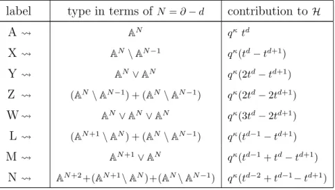
![Table 6.8: Dimensions and deviations for R = C[[z4 , z6 + z7]] , ` = 0 :](https://thumb-us.123doks.com/thumbv2/123dok_us/8276290.2191849/61.918.232.683.384.1085/table-dimensions-deviations-r-c-z-z-z.webp)
