Modeling oxygen dynamics and predicting hypoxic conditions in the
Neuse River Estuary, North Carolina
By
Nathalie H. Eegholm
Senior Honors Thesis Department of Biology
University of North Carolina at Chapel Hill
December 5th, 2018
Abstract
1. Introduction
Bodies of water all over the world are plagued by oxygen depletion, a problem that has been increasing in recent years (Testa et al. 2014). These conditions are known as hypoxia for dissolved oxygen (DO) concentrations below 2 mg/L. Once concentrations reach 0 mg/L, the conditions are classified as anoxic. Both conditions have severe consequences for aquatic vegetation and wildlife that need oxygen to survive (Testa et al. 2014). Often, low DO conditions arise due to the inhibition of oxygen supply from more oxygenated surface waters to the bottom waters due to suppression of vertical mixing by density stratification. If the rate of consumption of oxygen exceeds the rate of reoxygenation, hypoxic conditions are common (Diaz 2001). The complex interactions of various biogeochemical and physical processes work together to cause hypoxia (Fig. 1).
Figure 1. Diagram detailing factors that cause hypoxia, including density stratification and
eutrophication.
productivity could initially be beneficial for the food web by supplying energy and nutrients to lower trophic level organisms, there is a point at which the balance of the ecosystem is altered (Diaz 2001). Algal blooms often lead to hypoxia because the decomposition of the algal biomass and other organic matter by bacteria is an oxygen-intensive process (Paerl et al. 1998; Borsuk et al. 2001). Hypoxia will likely become a much greater and more widespread problem as a result of human impacts, including an increase in anthropogenic nutrient loading which will intensify eutrophication. Strong variations in DO that occur over short timescales of just a few hours are especially devastating to many organisms (Reynolds-Fleming & Luettich 2004). While some organisms may able to relocate to avoid low DO conditions, oftentimes in wind-driven systems, they are caught in low DO water that has been rapidly and recurrently upwelled as a result of episodic and sudden changes in wind direction and speed (Reynolds-Fleming & Luettich 2004). Sessile organisms, such as bivalves, are unable to avoid these conditions and may perish if exposed to prolonged hypoxic conditions. The entrapment of fish and sessile organisms within hypoxic water can cause physiological stress that results in lowered growth and reproduction rates (Breitburg 2002). Additionally, oysters subjected to diel-cycling hypoxia have been shown to be more subject to diseases such as Perkinsus marinus, otherwise known as “Dermo” (Breitburg et al. 2015). Another impact of hypoxia is mass die-offs of fish that can impair recreation and fishing. In the Neuse River Estuary (NRE) of North Carolina, fish kills usually impact species such as menhaden, striped bass, croaker, and flounder. Of the fish kills investigated in 2016, most were attributed to hypoxic conditions experienced in the summer (Young 2016). Such changes in habitat, predator-prey dynamics, and stress on various aquatic organisms can have detrimental cascading effects. The growing problem and relative unpredictability of hypoxia has made it a topic of focus for many modeling studies, the models of which can be implemented to help determine whether nutrient reduction goals and policies will be effective in supporting water quality, including the availability of DO (Scavia et al. 2006).
separates the bottom water column from the more oxygenated upper water column (Lowery 1998). Elevated temperatures during the summer increase metabolic rates and respiration of organisms, such as phytoplankton and microbial bacteria (Stanley & Nixon 1992; Buzzelli et al. 2002). However, increased hypoxia prevalence during summer is not necessarily the case for all systems, as stratification in salinity-stratified systems may depend more on wind speed, direction, and fetch, as well as freshwater inflow (Codiga 2012). In estuaries, density stratification of the water column is mostly the result of a vertical salinity gradient. This gradient can become intensified during periods of weaker winds or winds of a direction that force fresher water over more saline water, thus increasing vertical salinity stratification (Scully 2013; Geyer 1997). The salinity and density gradients also strengthen in the event of large freshwater inflows to the system. Scully (2013) created a three-dimensional circulation model linked to a biogeochemical model that assumed constant biological oxygen consumption. The model demonstrated clear seasonal and interannual cycling of hypoxia and reproduced observed DO levels well, indicating that physical forcing is very important in driving patterns in hypoxia and must be included in models.
of a simple model to predict variations in DO concentrations that occur over short timescales, specifically in the wind-driven Neuse River estuary (NRE). The goal of the creation of a simpler and more accessible model is to increase the basic understanding of mechanisms that drive hypoxia and to help make policy and management decisions surrounding this issue.
The basis and starting point for the study was a simple box model, which was developed to simulate DO levels over seasonal and yearly timescales using biweekly data (Borsuk et al. 2001). We applied the model to the NRE and compared the results with depth profiles of salinity, temperature, and DO data collected every 30 minutes to understand DO variability in the NRE and to assess the ability of the Borsuk model to describe DO variations on shorter timescales, on the order of hours to days. Understanding the limitations of the model will allow us to improve upon the model, with the goal of being able to forecast hypoxic events and potential fish kills that can impact ecosystem health as well as ecosystem services, including recreation and fishing.
2. Methods
2.1Study Site
The Neuse River originates in Durham, NC and flows almost 320 km to the Pamlico Sound (Borsuk et al. 2001). The estuary reaches around 70 km from the sound to just north of New Bern. Although long, the estuary is shallow, with an average water depth of just under 4 m (Luettich et al. 2001). As the presence of barrier islands off the coast of North Carolina limit tidal influence (Fig. 2a), most of the vertical mixing of the water columns is due to wind forcing (Borsuk et al. 2001). While the NRE is usually classified as a partially-mixed estuary, in reality, the system is quite variable, as wind forcing, depending on direction, speed, and duration, can mix the water column thoroughly or cause extreme stratification (Luettich et al. 2001).
2.2 Dataset
dataset includes vertical profiles of dissolved oxygen, temperature, and salinity measured by a multi-parameter sonde (YSI EXO2) mounted on a floating Autonomous Vertical Profiler (AVP) platform, and time series of salinity, temperature, and dissolved oxygen at fixed heights from a nearby conductivity, temperature, and depth (CTD) device (Seabird SBE37-SMP-ODO) chain. The AVP data used for this part of the project consists of vertical profiles of key variables (salinity, temperature, and DO) measured once every 30 minutes, at 10 cm depth intervals from the surface of water down to 6 m depth. These same variables were measured at fixed heights above bottom by three CTDs at the approximate top, middle, and bottom of the water column. The average depths for the CTDs top, middle, and bottom measurements were 1.61 m, 3.46 m, and 5.32 m, respectively.
Figure 2a, b. a) Overview of eastern North Carolina. The Neuse River Estuary is highlighted in
2.3 Data analysis
The CTDs provide stable, accurate conductivity, temperature, and depth measurements, while sonde measurements are less accurate and more susceptible to drift. The AVP and CTD data were compared to assess whether the sonde was well calibrated. This was done by plotting the measurements for variables for each dataset, at comparable heights above bottom, against each other. Linear regressions were performed and the slope of the regression lines and R2 values were used to assess the quality of the sonde calibration. There was a strong correlation between the AVP data and the CTD data, for all three variables: salinity, temperature, and dissolved oxygen concentration. The majority of the data points fell close to the 1:1 line. The slopes were close to 1.0, suggesting that the sonde was well calibrated. This validation justified the use of the AVP data throughout the rest of the project. This was beneficial because the AVP data contained more data points and greater vertical depth resolution than the CTD data.
Statistical relationships between DO and other variables were assessed to obtain a better understanding of what drives DO dynamics within the NRE. This was done by plotting DO versus key parameters that affect dissolved oxygen levels. The water column during the time period studied was strongly stratified and showed two distinct layers throughout most of the measurements. Therefore, the profiles were split into two layers for analysis. For the bottom layer, DO was plotted against water temperature and against the difference in salinity between the two layers, which is a measure of the strength of the density stratification. We then performed linear regressions on the data to determine if there were any relationships between these variables.
2.4 Model
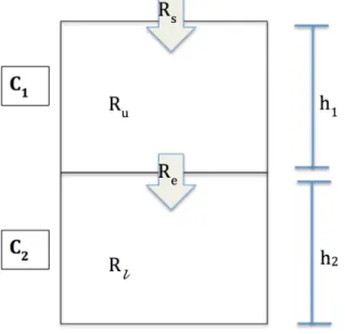
The dissolved oxygen model was based on the two-layer box model introduced by Borsuk et al. (2001). The model aims to calculate the evolution of the DO concentration in the upper layer, C1, and in the bottom layer, C2 (Fig. 3) as the result of consumption in the lower
oxygen consumption and the effects of physical reoxygenation (Borsuk et al. 2001). The model assumes that horizontal advection of oxygen is negligible compared with atmospheric exchange, exchange via mixing between the two layers, and consumption by biogeochemical processes.
Figure 3. A diagram of the model and its parameters. C1 and C2 are the concentrations of DO in
the upper and lower water layers, whose heights are represented by h1 and h2, respectively. Ru
and Rl are the sources of DO in the upper and lower water layers, respectively. The Rs term is
the surface water-air exchange of DO. The Re term is the vertical exchange rate between the two
layers. The directions of the arrows indicate the directions for which Rs and Re were defined as
positive.
The differential equations 1 and 2, express the concentrations of DO in the upper and lower water layers, respectively, in terms of the model shown in Figure 3.
!!!
!"
=
𝑅
!+
!!!!
−
!!
!!
!!!
!"
=
𝑅
!+
!!!!
(1)
In the Borsuk model, the DO concentration of the top layer is assumed to be equal to the DO concentration at saturation, and is a function of temperature, T:
𝐶
!=
13
.
686
∗
0
.
34663
𝑇
+
0
.0045
𝑇
!Equation 3 assumes an average salinity of 10 PSU. The DO concentration in the lower layer was computed from the conservation equation:
!!!
!"
=
−𝑘
!𝐶
!+
!!!
!!!∆! !!
(
𝐶
!−
𝐶
!)
The two terms on the right side of Equation 4 represent the rate of consumption of DO in the lower water layer and the exchange rate between the two layers, respectively. In this parameterization, kd is the rate constant (d-1), k’v is the vertical exchange coefficient (d-1), ΔS is
the difference in salinity between the top and bottom layer (PSU), and b is a constant.
2.5 Application of model to Neuse dataset
In this project, the model described by Equations 1-4 was implemented in MATLAB and applied to the dataset from June to July of 2016. Measured DO concentrations in the top layer were compared to values predicted by Equation 3. As agreement was poor at the timescales of interest in this study, we used the top layer DO concentrations measured by the AVP for C1 in the
model to predict the bottom layer concentration, C2.
The focus of the project was to understand the Borsuk model for the bottom water DO concentration because it was biologically the more interesting problem. The lower layer DO concentration at the beginning of each time period of interest (the initial condition) was set to equal the measured concentration at that time. The ordinary differential equation in Eq. 4 was
then solved numerically using a forward difference in time (Euler method). The measured salinity difference between the two layers at each timestep was used for ΔS.
We wanted to see how well the model performed at reproducing higher frequency data, and data that had been smoothed (time-averaged) to different degrees. In order to reduce the noise in the data, we performed a 4-hour moving average and to remove diurnal cycling, we performed a 24-hour smooth moving average on the data for DO, temperature, and salinity.
To investigate the behavior of the model in more detail, we selected three distinct events from the time period. Event 1 was defined as the period from June 22-25, 2016, and Event 2 was defined as the period from June 17-20, 2016. Event 1 was a stratification event, where the water column changed from well mixed to stratified. Event 2 was a mixing event, in which the water column transitioned from stratified to well-mixed. Using these events, we conducted sensitivity analyses to understand how the Borsuk model would respond to varying different parameters. This allowed us to explore the consumption and vertical mixing terms separately to understand the effect of each term on the prediction of bottom DO.
We began by assessing the model’s accuracy using the parameter ranges outlined in Borsuk et al. 2001. The median estimated values for kd, k’v, and b were 0.113, 0.052, -0.012,
respectively (Borsuk et al. 2001). In our sensitivity analysis, we plotted consumption and vertical mixing terms calculated from values of kd and k’v that were doubled these median values. In
addition, we plotted consumption and vertical mixing terms calculated for values of kd and k’v
that were 0.5, an arbitrary value.
3. Results
3.1 Conditions during the measurement period
Periods of moderate winds to the northeast are correlated with strengthening water column stratification. This is reasonable, as winds toward the northeast would force fresher water over the saline Pamlico Sound water and increase the stratification, creating conditions that prevent mixing and cause low concentrations of DO in the lower water column. Winds to the southwest coincide with periods of decreasing stratification, consistent with increased mixing as denser more saline water is forced up the estuary in the upper water column. Of the 27 days in the time period between June 8 and July 4, 2016, 16 unique days experienced some bottom water hypoxia. Of all the time points in the data set, bottom water was hypoxic 24.33% of the time.
Figure 4a, b, c, d. Variation of a) salinity, b) temperature, and c) DO vertical profiles over time
3.2 Statistical relationships between variables
Bottom layer temperature and bottom water DO were not correlated (Fig. 5a), indicating that there was not a significant increase in biological oxygen demand with increasing temperature over the observed bottom temperature range (25.3-28.5 °C). There is, however, a moderate correlation between salinity stratification, defined as the salinity difference between the upper and lower layers, and bottom layer DO (Fig. 5b). Generally, as salinity stratification increases, bottom layer DO decreases.
Figure 5a, b. a) Relationship between bottom water layer DO and bottom layer temperature and
b) difference in salinity between the two layers. The orange line in panel b is the linear regression of DO against salinity difference. At the top right corner of each plot is an R2 value indicating goodness of fit.
25 25.5 26 26.5 27 Bottom Water Temperature (C)
0 1 2 3 4 5 6 7 8
Bottom Water Dissolved Oxygen (mg/L)
-2 0 2 4 6 8 10 Delta Salinity (PSU)
-2 -1 0 1 2 3 4 5 6 7 8
R-squared: 0.636 R-squared: 0.097
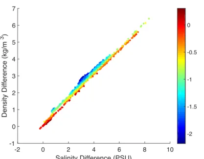
Figure 6. Layer density difference as a result of the layer salinity difference, where each point is colored by the layer temperature difference.
Differences in density between the two layers can be attributed mostly to differences in salinity. Differences in density and salinity between the two water layers were strongly related, with an R2 value of 0.989. The slight variations in density that are not accounted for by salinity are attributed to temperature differences (Fig. 6). For greater differences in layer temperature, there were greater density differences between the layers.
3.3 Application of the Borsuk Model
The Borsuk model was not able to reproduce observed patterns in top layer DO concentration (Fig. 7). The equation given in the Borsuk paper to calculate the top water layer DO concentration (Eq. 3) assumes DO to be at saturation, calculated from temperature values, and assumes an average salinity of 10 PSU. The values computed using Equation 3 have peaks and valleys in the opposite direction from the actual AVP top layer DO data, suggesting that the assumption that the upper layer DO concentration is in equilibrium with the atmosphere over the resolved timescales is poor. Given this, we used the upper layer DO concentrations measured by the AVP for C1 in the model to predict the lower layer concentration C2.
-2 0 2 4 6 8 10
Salinity Difference (PSU)
-1 0 1 2 3 4 5 6 7
Density Difference (kg/m
3 )
Figure 7. Time series of upper water layer DO concentration (mg/L). The blue line is the actual upper layer DO concentration, and the red line represents C1, the upper layer DO concentration modeled using Equation 3.
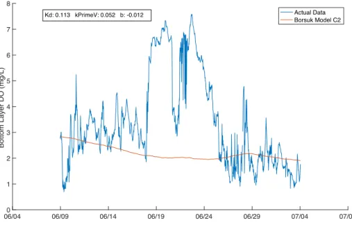
Figure 8. Time series of bottom water layer DO concentration (mg/L). The blue line is the actual
bottom layer DO concentration, and the red line represents C2, the bottom layer DO concentration modeled using Equation 4 using the median values for the parameters as stated in
06/040 06/09 06/14 06/19 06/24 06/29 07/04 07/09 1
2 3 4 5 6 7 8
Bottom Layer DO (mg/L)
Actual Data Borsuk Model C2 Kd: 0.113 kPrimeV: 0.052 b: -0.012
06/045 06/09 06/14 06/19 06/24 06/29 07/04 07/09 5.5
6 6.5 7 7.5 8 8.5 9
Top Layer DO (mg/L)
Our implementation of the bottom layer model for C2 indicates that the modeled and
measured bottom layer DO concentration were not in agreement for the median parameter values proposed in Borsuk (2001) (Fig. 8). The model does not capture the DO variations that are present in the data. The model does not capture the increase in bottom DO that occurs between June 19, 2016 and June 24, 2016. This information led us to look at the data on smaller timescales, for the three events defined in Methods.
Figure 9a, b, c, d. DO concentrations over time for Event 1 (a) and Event 2 (c). Salinity difference over time for Event 1 (b) and Event 2 (d). In plots a, and c, the top layer DO concentrations are plotted in dark blue, red, and yellow, indicating non-smoothed data, 4-hour smooth moving average, and 24-hour smooth moving average, respectively. In plots a and c, the bottom layer DO concentrations are plotted in purple, green, and light blue, indicating non-smoothed data, 4-hour smooth moving average, and 24-hour smooth moving average, respectively. In plots b and d, the salinity difference between the layers is plotted in dark blue, red, and yellow, indicating non-smoothed data, 4-hour smooth moving average, and the 24- hour
a
06/220 06/23 06/24 06/25 06/26 1 2 3 4 5 6 7 8 9 DO (mg/L)
non-smoothed Top DO 4 hr SMMA Top DO 24 hr SMMA Top DO non-smoothed Bottom DO 4 hr SMMA Bottom DO 24 hr SMMA Bottom DO
06/220 06/23 06/24 06/25 06/26 1 2 3 4 5 6 7 8 9
Salinity Difference (PSU)
non-smoothed 4 hr SMMA 24 hr SMMA
06/170 06/18 06/19 06/20 06/21
1 2 3 4 5 6 7 8 9 DO (mg/L)
06/170 06/18 06/19 06/20 06/21
1 2 3 4 5 6 7 8 9
Salinity Difference (PSU)
c d
Figure 10a, b, c, d. Plots of rate of change of bottom water DO concentration (dC2/dt) over time for Event 1 (a, b) and Event 2 (c, d). The blue line on each plot represents the dC2/dt for each event. The yellow, purple, and green lines in panels a and c show the effects on dC2/dt for different values of kd, the consumption coefficient (Eq. 4), for a k’v (vertical exchange coefficient,
denoted in plots as “kv”) value equal to the median value proposed in the Borsuk model. The yellow, purple, and green lines in panels b and d show the effects on dC2/dt for different values of k’v, for a kd value equal to the median value proposed in the Borsuk model. In all cases, the
constant b was the median Borsuk value of -0.012. 06/22 06/23 06/24 06/25 06/26 -4 -3 -2 -1 0 1 2 3 dC2/dt dC2/dt
vertical mixing, kv=0.052 kd=-0.113
kd=-0.226 kd=-0.5
06/22 06/23 06/24 06/25 06/26 -4 -3 -2 -1 0 1 2 3 dC2/dt dC2/dt consumption, kd=-0.113 kv=0.052 kv=0.104 kv=0.5
06/17 06/18 06/19 06/20 06/21 -4 -3 -2 -1 0 1 2 3 4 5 dC2/dt dC2/dt
vertical mixing, kv=0.052 kd=-0.113
kd=-0.226 kd=-0.5
06/17 06/18 06/19 06/20 06/21 -4 -3 -2 -1 0 1 2 3 4 5 dC2/dt dC2/dt consumption, kd=-0.113 kv=0.052 kv=0.104 kv=0.5
c d
The values for the sensitivity analysis for the parameters kd and kv were chosen by
doubling the Borsuk median value for each parameter and arbitrarily assigning both values to be 0.5 for a third run (Fig. 10a-d). For increasingly negative values of kd, we saw a larger
consumption term, which was expected (Figs. 10a, c). Increasing the value of k’v increased the
magnitude of the vertical mixing term (Figs. 10b, d). In the case of increasing both parameter values, we noticed that there was still no parallel between the runs and the actual rate of change of C2, as the patterns of each did not match. It appears that the vertical mixing term varies with
(C1-C2), as in Equation 4, so the vertical mixing term is larger when the water column is
stratified. Likewise, it is smaller when the water column is well-mixed. This does not capture the pattern of decreasing mixing with increasing stratification.
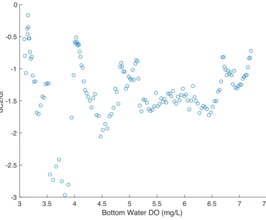
Figure 11. The rate of change of bottom DO for Event 1 vs. bottom DO concentration (C2).
3 3.5 4 4.5 5 5.5 6 6.5 7 7.5
Bottom Water DO (mg/L)
-3 -2.5 -2 -1.5 -1 -0.5 0
Because the consumption term of Equation 4 is dependent on the bottom DO concentration, we plotted the rate of change of C2 versus the bottom DO values for Event 1, a
stratification event, in which the effects of consumption of DO is more profound than the replenishment by vertical mixing. The form of the consumption term in Equation 4 assumes that the rate of consumption (dC2/dt) varies linearly with C2. From our analysis this is not the case,
and instead dC2/dt appears to have a constant value independent of C2 (Fig. 11). There is
therefore no constant value of the kd rate coefficient that would be suitable for modeling changes
in bottom DO during this event.
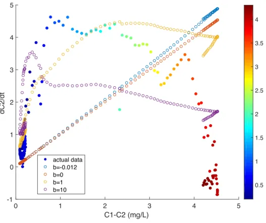
Figure 12. Rate of change of bottom DO concentration vs. layer DO concentration difference
(mg/L), with each point colored by bottom water salinity (PSU), for Event 2 (mixing event). The blue line represents the vertical mixing term for the median Borsuk value, b=-0.012 and k’v =1.
The red line represents the vertical mixing term for b=0 and k’v= 1. The yellow line represents
the vertical mixing term for b=1 and k’v = 10. The purple line represents the vertical mixing
term for b=10 and k’v = 100.
0 1 2 3 4 5
C1-C2 (mg/L)
-1 0 1 2 3 4 5
dC2/dt
actual data b=-0.012 b=0 b=1
b=10 0.5
Similarly, we studied the vertical mixing term separately. Because the vertical mixing term of Equation 4 is dependent on the difference in DO concentration between the top and bottom layers (C1-C2), we plotted the rate of change of C2 versus C1-C2 for Event 2, a mixing
event. We expect in Event 2 that the effects of vertical mixing of DO dominate over consumption. Instances of greater DO difference between the layers are strongly correlated with a greater salinity gradient. The rate of change of bottom DO concentration is low when the concentration difference between layers (C1-C2) is small, which also corresponds to small
salinity gradient (ΔS). The rate of change of bottom DO increases as C1-C2 and ΔS increase, until
a certain point, beyond which it then decreases again for highly stratified systems (Fig. 12). The form of Equation 4, however does not take this into account, as the value of dC2/dt should increase linearly for larger values of k’v, and does not eventually decrease for increasing
conditions of stratification.
4. Discussion
4.1 Dissolved Oxygen Dynamics in the NRE
While temperature did not vary a great deal over the data utilized in this study, the water column was intermittently mixed and stratified due to salinity differences. Bottom water hypoxia occurred approximately a quarter of the days in the dataset, indicating that this is a fairly severe issue in the NRE. Because the NRE is often stratified, we divided the system into two distinct layers in our analysis. We saw large variations in DO differences between the layers, which we were able to attribute to periods of large and small salinity gradients (Fig. 5b). We saw a strong relationship between bottom water DO and difference in salinity between the two layers, suggesting that physical processes, especially stratification, are major factors in controlling bottom water DO.
4.2 Borsuk Model, C1
equation used to predict the DO concentrations in the top water layer was not able to reproduce the DO variations observed in our dataset. While we expected that the model would not be able to completely predict the DO variations, we found that it showed quite different trends (Fig. 7). The difference in the peaks and troughs suggests that biological drivers, such as respiration and photosynthesis, have a larger effect on upper water column DO than saturation does. This information led us to use the upper layer DO concentrations measured by the AVP for C1 in the
model to predict the lower layer concentration C2. Further work is needed to develop a model
that can predict upper water column DO variations, and our work suggests that any such model would need to include representations of the biological processes of photosynthesis and respiration, which may depend on salinity, which is currently unaccounted for in Equation 3.
4.3 Borsuk Model, C2
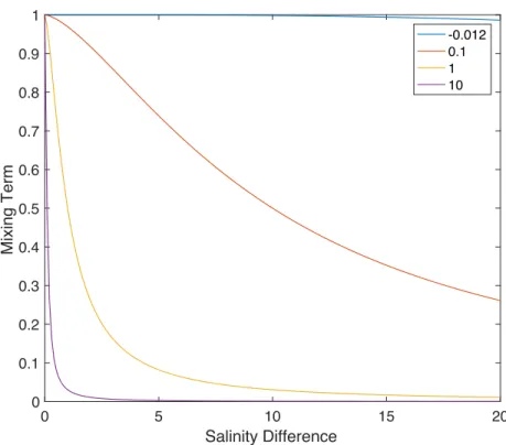
From our sensitivity analysis, it is evident that the patterns in the vertical mixing terms do not follow the pattern in the dC2/dt data (Figs. 10 c, d). The term seems to increase as a result of the difference in DO between the layers, and seems to be relatively unaffected by the decrease in density stratification that we see over the course of Event 2. This prompted investigation into the behavior of the vertical mixing term further. We look at an important constant that as defined as b, which is related to a constant of proportionality related to the ratio between a simple relationship between buoyancy and shear (Borsuk et al. 2001). The range of salinity differences between the top and bottom water layers for this study was between 0 and 8.3 PSU. Over this range, the chosen median value for b, -0.012, in the Borsuk study would not have any effect on the mixing term of Equation 4 (Fig. 13). One way to estimate the salinity difference at which mixing would be suppressed is to consider the bulk Richardson number, Rib, which represents
the ratio of energy needed to mix the water column to energy available in the flow to generate turbulence (Kundu 1990).
(5)
In Equation 5, g is acceleration due to gravity, ρ0 is average density, Δz is interface
2 0
b
i
u
g z
R ρ
ρ
Δ Δ
Δ
critical value of 0.25, there is sufficient energy to mix the water column and shear dominates over stratification (Kundu 1990). For the highest shears in this study (Δz ~ 1 m, Δu = 0.3 m/s),
Rib = 0.25 when Δρ ~ 2 kg/m3. This corresponds to a ΔS of approximately 3 PSU (Fig. 6). For
smaller shear values observed in this study (Δz ~1 m, Δu ~ 0.1 m/s), Rib = 0.25 when Δρ ~ 0.25
kg/m3, which corresponds to a ΔS of about 0.3 PSU (Fig. 6). We varied the parameter b and
examined the resulting dependence of the vertical mixing term on the salinity difference between the two layers (Fig. 13). To achieve suppression of the mixing term at ΔS between 0.3-3 PSU,
the parameter b should be between 1 and 10, and would vary depending on shear, which is variable in this system (Fig. 13).
Figure 13. Mixing term for constant C1-C2 vs. salinity difference (PSU) for different values of b.
The median value of b used in the Borsuk model, -0.012, has no effect on the vertical mixing term of Equation 4 over the salinity gradients that occurred in the NRE between June and July of 2016. By varying the values of b, we were able to see that higher orders of magnitude (i.e. 1 and 10) did have an impact on the vertical mixing term (Fig. 13). The vertical mixing term
0 5 10 15 20
Salinity Difference 0
0.1 0.2 0.3 0.4 0.5 0.6 0.7 0.8 0.9 1
Mixing Term
of Equation 4 could be improved by the use of a more representative b value to better model the changes in DO that occur in the stratification conditions we see in the data.
4.4 Future Directions
Our analysis has shown that the Borsuk model does not accurately portray DO variations at the timescales of the data we utilized. This is likely due to the aforementioned model being designed to predict the average over many conditions, to show broad patterns at seasonal and interannual timescales. This does not translate well in terms of predicting high frequency processes. The model should be further developed by analyzing individual events. This will aid in the development of terms that can accurately represent the processes occurring over these shorter timescales and describe DO variability in this system. Then the model could potentially be applied to larger datasets that span longer periods of time. It will be necessary to work with high frequency data for more months of the year and over multiple years in order to take this study further. In addition, future models must take into account flow, which is important at these timescales of hours and days, because it can vary greatly even within the same system. For example, wind conditions are important in dictating flow and mixing conditions. This model would be useful to combine with other models that detail biogeochemical oxygen demand to get a better view of the factors that control DO variability in the NRE, which could help assess the impact of nutrient management techniques to reduce eutrophication. Subsequently, this model could be applied to the rest of the data that was collected from 2016 in order to see if the model proves to be effective in hindcasting hypoxia in the NRE for that period. This would pave the way for using the model to forecast shorter frequency variation in DO.
Acknowledgements
I would like to thank my research advisor Dr. Johanna Rosman for all her expertise and help and invaluable guidance throughout the project. I want to recognize Dr. David Marshall for his assistance, as well as the Luettich Lab at UNC IMS for collecting the AVP data. I would also like to thank Dr. Amy Maddox of UNC for serving as the Biology Sponsor for this project. Furthermore, I would like to acknowledge Sarah McQueen for providing helpful feedback and being a great writing partner.
References
Borsuk ME, Stow CA, Luettich RA, Paerl HW, Pinckney JL. 2001. Modelling oxygen dynamics in an intermittently stratified estuary: estimation of process rates using field data. Estuarine, Coastal and Shelf Science, 52. doi:10.1006/ecss.2000.0726.
Breitburg DL. 2002. Effects of hypoxia, and the balance between hypoxia and enrichment, on coastal fishes and fisheries. Estuaries, 25.
Breitburg DL, Hondorp D, Audemard C, Carnegie RB, Burrell RB, Trice M, Clark V. 2015. Landscape-level variation in disease susceptibility related to shallow-water hypoxia. PLOS one, doi: 10.1371/journal.pone.0116223.
Buzzelli CP, Luettich RA, Powers SP, Peterson CH, McNinch JE, Pinckney JL, Paerl HW. 2002. Estimating the spatial extent of bottom-water hypoxia and habitat degradation in a shallow estuary. Marine Ecology Progress Series, 230. doi:10.3354/meps230103.
Codiga DL. 2012. Density stratification in an estuary with complex geometry: driving processes and relationship to hypoxia on monthly to inter-annual timescales. Journal of Geophysical Research-Oceans 117. doi: 10.1029/2012JC008473.
Diaz RJ. 2001. Overview of hypoxia around the world. Journal of Environmental Quality, 30(2).
Geyer WR. 1997. Influence of wind on dynamics and flushing of shallow estuaries. Estuarine, Coastal and Shelf Science, 44.
Kundu PK. 1990. Fluid Mechanics, Academic Press, San Diego, Calif.
Lowery TA. 1998. Modeling estuarine eutrophication in the contest of hypoxia, nitrogen loadings, stratification and nutrient ratios. J. Environmental Management, 52.
and productivity, sedimentary processes and benthic-pelagic coupling, and benthic ecology. Water Resources Research Institute News of the University of North Carolina, 327.
Paerl HW, Pinckney JL, Fear JM, Peierls BL. 1998. Ecosystem response to internal and watershed organic matter loading: consequences for hypoxia in the eutrophying Neuse River Estuary, North Carolina, USA. Marine Ecology Progress Series, 166.
Peña MA, Katsev S, Oguz T, Gilbert D. 2010. Modeling dissolved oxygen dynamics and hypoxia. Biogeosciences, 7.
Reynolds-Fleming JV, Luettich RA. 2004. Wind-driven lateral variability in a partially mixed estuary. Estuarine, Coastal and Shelf Science, 60. doi:10.1016/j.ecss.2004.02.003.
Scavia D, Kelly ELA, Hagy JD. 2006. A simple model for forecasting the effects of nitrogen loads on Chesapeake Bay hypoxia. Estuaries and Coasts, 29(4).
Scully ME. 2010. Wind modulation of dissolved oxygen in Chesapeake Bay. Estuaries and Coasts, 33. doi: 10.1007/s12237-010-9319-9
Scully ME. 2013. Physical controls on hypoxia in Chesapeake Bay: A numerical modeling study. Journal of Geophysical Research: Oceans,118. doi:10.1002/jgrc.20138.
Stanley DW, Nixon SW. 1992. Stratification and bottom-water hypoxia in the Pamlico River Estuary. Estuaries, 15(3). doi:10.2307/135n2775.
Testa JM, Li Y, Li M, Brady DC, Di Toro D M, Kemp WM, Fitzpatrick JJ. 2014. Quantifying the effects of nutrient loading on dissolved O2 cycling and hypoxia in Chesapeake Bay using a coupled hydrodynamic–biogeochemical model. Journal of Marine Systems, 139. doi:10.1016/j.jmarsys.2014.05.018.