Thesis

(1)

An Assessment of Marine Hydrokinetic (MHK)

Energy in the Gulf Stream off Cape Hatteras,

North Carolina

Caroline Ford Lowcher

University of North Carolina at Chapel Hill

A senior honors thesis submitted in partial fulfillment of the requirements for a degree of Bachelor of Arts in Interdisciplinary Studies in Oceanography.

Department: Interdisciplinary Studies

Majors: Applied Mathematics Interdisciplinary Studies in Oceanography

Major Professor: Dr. John Bane

__________________________

Reader: Dr. Ruoying He

Reader: Dr. Harvey Seim

(2)

Acknowledgements

I am most appreciative of all the guidance given by my advisor, John Bane, and mentor, Mike Muglia. Mike who handed me the opportunity to get my feet wet not only in the field but also in the career as a scientific researcher, and for securing a job position giving me the freedom to immerse myself into this project and other coastal

oceanography research. He has shared with me the fun in doing science through his adventurous and love-of-life personality, and he has shared with me his ADCP data used in this thesis. John has kindly worked with me over the years I have spent at UNC not only as a professor but also as my advisor for my Interdisciplinary Studies in

Oceanography major. He has taught me much in physical oceanography, and it has been a pleasure and absolute joy to work with him on a daily basis. His expertise on the Gulf Stream has made him an invaluable asset to this thesis, and his experiences and wisdom have been most helpful in my future endeavors of graduate school. Without these two I would not have learned as much about oceanography, data analysis, and field work techniques, and owe my accomplishments of the past few years in this field to these two. Other individuals who were also influential and have helped me grow as a scientist are Ruoying He, Yanlin Gong, and Sara Haines. Ruoying and Yanlins’ support in

generously providing the model data with Sara’s help on data analysis tools has been essential to this thesis and with the subsequent work that will expand from it. This group of people has been most excellence and enjoyable to work with over the last few years, and I am hopeful for all that can come out of this group’s efforts.

(3)

LIST OF FIGURES

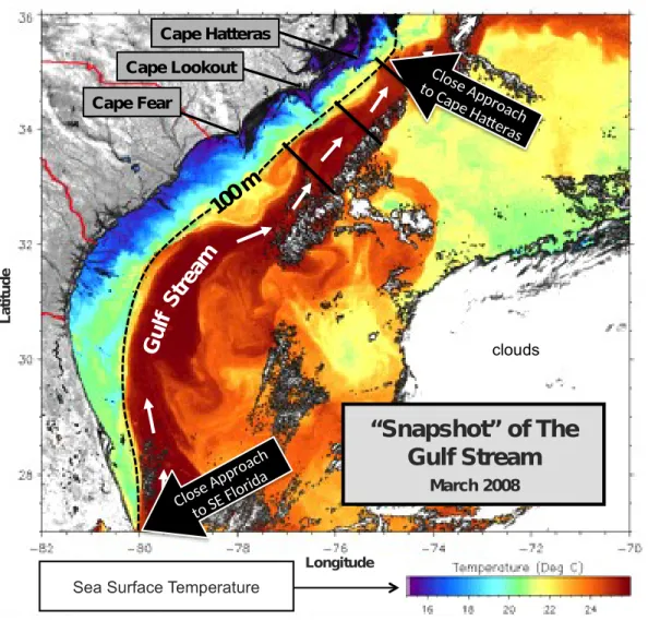
Figure 1. A sea surface temperature (SST) snapshot of the Gulf Stream along the US

southeast coastline in March 2008.

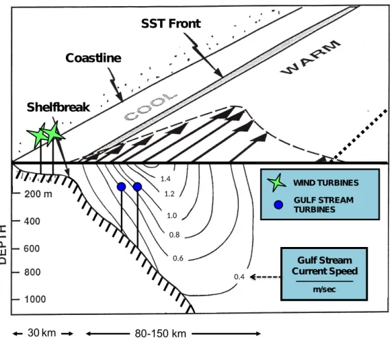
Figure 2. Gulf Stream schematic taking a vertical slice of the current.

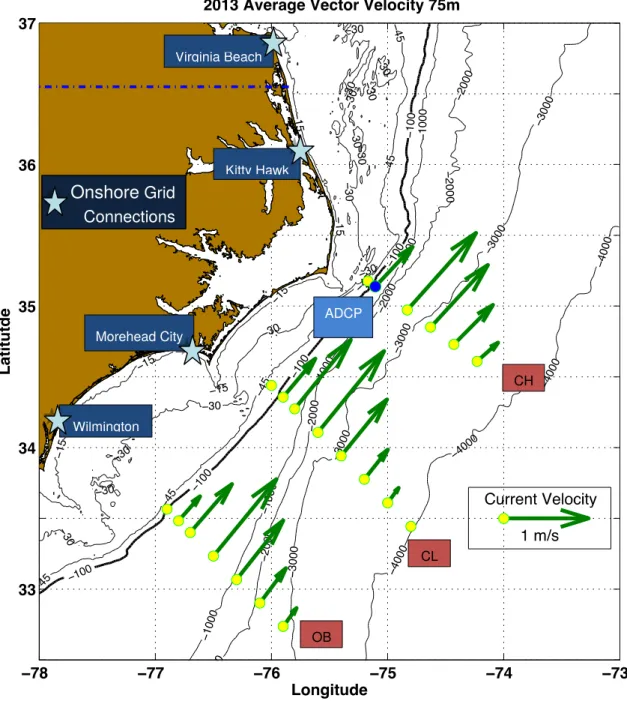
Figure 3. 2013 average current velocities at 75 m overlying a North Carolina base map.

Figure 4. Snapshot of the vertical slices at the three cross-isobath transects on November 1, 2013 using model data.

Figure 5. Time series of the current speed at 75 m from August 1, 2013 thru April 28,

2014.

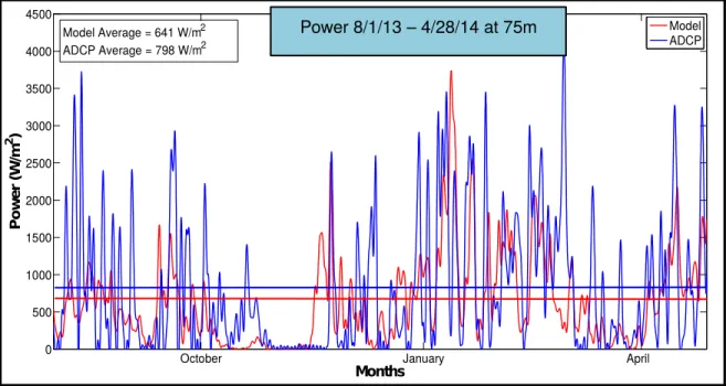
Figure 6. Time series of the power density at 75 m from August 1, 2013 thru April 28,

2014.

Figure 7. Five-year model annual power density averages from 2009 – 2013 at 75 m at

station 3 (ADCP location) in the Cape Hatteras transect.

station 3 in the Cape Lookout transect.

station 2 in Onslow Bay transect.

multiple stations in the Cape Hatteras transect. Red vertical bars of station 3 (ADCP location) are the same as those in Figure 6.

multiple stations in the Cape Lookout transect. Red vertical bars of station 3 are the same as those in Figure 7.

multiple stations in the Onslow Bay transect. Red vertical bars of station 2 are the same as those in Figure 8.

Figure 13. ADCP current rose from August 1, 2013 thru April 28, 2014 at 75 m.

Percentages show the time spent in a given direction.

Figure 14. Model current rose from August 1, 2013 thru April 28, 2014 at 75 m.

(5)

(6)

LIST OF TABLES

Table 1. Cape Hatteras Cross-Isobath Transect Stations

Table 2. Cape Lookout Cross-Isobath Transect Stations

(7)

ABSTRACT

The Gulf Stream is the western boundary current of the North Atlantic subtropical gyre, and it flows for part of its course just offshore of the southeastern US coastline. This large-scale ocean current has current velocities reaching approximately 2 m s-1_{, which}

distinguish it as a potential source of marine hydrokinetic (MHK) energy. The upper continental slope off Cape Hatteras is a desirable area for development of offshore renewable energy because of the narrowness of the continental shelf and the Stream’s minimal meanderings there. Using current data from a moored 150 kHz acoustic Doppler current profiler (ADCP) and from the Mid-Atlantic Bight and South Atlantic Bight (MABSAB) regional ocean circulation model, MHK power characteristics have been computed for this area. These calculations quantify the Gulf Stream power resource and its temporal and spatial variations. During August 2013 – April 2014 at the moored ADCP site and 75 m below the ocean surface, which was within the Gulf Stream’s cyclonic shear zone, a comparison of the ADCP and MABSAB model currents reveals that the average current speeds from the two sources are nearly identical, with a magnitude of 0.94 m s-1_{. A comparison for the same time period was made for the}

current’s power density. The ADCP-observed average was 798 W m-2_{, and the model}

average was 641 W m-2_{, a difference of about 20%. The model has shown to have similar}

current speeds to the ADCP for slowly varying currents (fluctuations of weeks to months), and lower speeds for higher frequency current variations (fluctuations of several days to a couple of weeks). The model also shows somewhat less variability than the ADCP in directionality of the Stream’s flow. Model data have been used to calculate the annual power density averages for a number of years at various locations within the Gulf Stream over the North Carolina continental slope. These results show the variation of the Stream's position along the North Carolina coastline over 2009-2013, and show that yearly averaged power at a given location has significant inter-annual variations. This holds true for the ADCP location where the model has an average power of 14 W m-2_in

(8)

Section 1: INTRODUCTION

Using technologies that are commercially available today, the National

Renewable Energy Lab (NREL) reported that 80% of US electricity generation in 2050

could sufficiently come from renewable energy resources (Renewable Electricity Futures

Study). Such resources include biomass, geothermal, hydrothermal, solar, and wind. Not

considered in this 80% is electricity generated by the ocean, due to a lack of technology

presently available for large-scale commercialization. However, what is the possibility

that ocean energy could be an adequate and cost-effective source for US electricity

generation?

Using large-scale currents for ocean energy was an idea that first rooted in the

1970s with the Coriolis program (Lissaman and Radkey, 1979; Stewart, 1974). The idea

was that a large turbine could be deployed in the Florida Current to harness energy for

commercial use. While this never developed in full scale, other studies have been done

to improve the speed and power estimates made in Lissaman and Radkey, 1979, and to

look at the power potential from the Gulf Stream using numerous ocean models. Yang et

al., 2013 estimated 44 GW to be the maximum energy dissipation by turbines using an

analytical approach to a simplified ocean circulation model, but Yang et al, 2014 now

used a numerical approach to look at the theoretical extractable power and found that the

range of average power dissipation was 4 to 6 GW with a mean of 5 GW. The results of

the second study demonstrate that a numerical approach may provide better estimates of

the obtainable power potential. While this is a large reduction in power from the initial

estimate, this is still a sizeable amount and could be used to support electricity demands

(9)

This thesis provides an assessment of the MHK energy off of North Carolina near

Cape Hatteras, near Cape Lookout, and in Onslow Bay. It analyzes how observational

measurements from a 150 kHz ADCP compare to a ROMS (Regional Ocean Model

System) model, and examines the power density over spatial and temporal domains.

These analyses provide estimates for how much power can be expected at locations off

the coastline, and should be used to determine which areas off of North Carolina are

optimal for deploying future MHK devices. The power estimates here do not include

technological constraints and frictional losses such as turbine efficiency and turbine

performance coefficients, which are described in Gorban et al., 2001, Guney, 2011, and

Hanson et al., 2014; however, these parameters strongly affect the extractable power that

(10)

Section 2: BACKGROUND

Western boundary currents like the Gulf Stream, Kuroshio, Brazil Current, and

Agulhaus Current are some of the fastest, large-scale ocean currents in the world and are

thus, of interest in terms of MHK energy. Driven by the Westerly and trade winds, the

Gulf Stream attains speeds greater than 2 m s-1₍_{Hanson et al}_{., 2011). The Gulf Stream is}

obvious in satellite sea surface temperature (SST) images, more so in the winter, less so

in the summer when the surrounding South Atlantic Bight (SAB) and Mid-Atlantic Bight

(MAB) shelf waters have similar SSTs to those in the Stream. The MAB is the

continental shelf off of the US east coast that extends from Cape Cod to Cape Hatteras,

and the SAB is the shelf from Cape Hatteras to Florida. The areas of the MAB and the

SAB that lie off of North Carolina and extend down to Florida are shown in Figure 1.

Due to the narrowness of the continental shelf off of Florida and North Carolina, the Gulf

Stream approaches closest to the southeast coastline in the Florida Straits and off of Cape

Hatteras. The inshore edge of the Gulf Stream is about 20 kilometers (~12.5 miles) off

the coastline near Cape Hatteras (Figures 1 and 3). Thus the proximity of the Stream to

the US coastline makes this area off of North Carolina of interest for MHK energy. As

part of the North Atlantic subtropical gyre circulation, the Gulf Stream flows through and

exits the Florida Straits. It then flows along the upper continental slope throughout the

SAB. At about 32° N latitude, the current encounters the Charleston Bump, where it

deflects offshore as it passes over the Bump (Brooks and Bane, 1978; Legeckis, 1979).

The current continues to flow northeastward, and off of the Carolinas meanders in the

path of the Gulf Stream grow in lateral amplitude as they propagate to the northeast. As

(11)

et al., 1981; Tracy and Watts, 1986). The meanders are the movements of the Stream

onshore and offshore, and this is one reason why the Gulf Stream may not be observed at

certain times by a fixed-position moored instrument. At around 36° N, the Gulf Stream

separates from the continental margin and flows northeastward as part of the North

Atlantic subtropical gyre. These processes are illustrated in Figure 1.

The Gulf Stream is about 100 kilometers wide and extends down to about 1

kilometer depth, as marked in Figure 2. The Stream has a jet structure, with fastest

speeds in its core at the surface of the current, and speeds decreasing in all directions

away from the core (Halkin and Rossby, 1985). Roughly one third of the inshore portion

of the Gulf Stream comprises the current’s cyclonic shear zone, and the remaining

portion along the offshore edge is the anticyclonic shear zone (Halkin and Rossby, 1985).

With regards to alternative ocean energy, wind turbines would typically be placed

up on the continental shelf and Gulf Stream subsurface turbines would be located on the

upper portion of the continental slope (Figure 2). The turbines or instruments

implemented would need to remain out of the way of ship traffic and below the wave

field to reduce wave-induced stress on the mooring hardware and turbines. Thus, the top

(12)

Section 3: METHODS

The Gulf Stream power analysis presented here uses data sets from two different

sources. One is the ROMS (Regional Ocean Model System) that has been run for an area

that encompasses the Cape Hatteras region. The other is from a 150 kHz ADCP (acoustic

Doppler current profiler) that was moored in the ocean on the upper continental slope off

Cape Hatteras. Each data source is described below.

3.1 ROMS Model

The ROMS model is called MABSAB (Mid-Atlantic Bight South Atlantic Bight),

and is run by Ruoying He’s research group at North Carolina State University. It has

outer ocean boundaries forced by HYCOM (Hybrid Coordinate Ocean Model), uses

NARR (North America Regional Reanalysis) for atmospheric forcing, and has sigma

coordinates that follow a free surface terrain (Shchepetkin and McWilliams, 2005). The

model is a hindcast and has 2 km horizontal spatial resolution with 36 vertical

terrain-following layers. Bathymetry in the model is interpolated from the National Geophysical

Data Center 2-Minute Gridded Global Relief Data. MABSAB does not incorporate the

observations from the ADCP into the model computations of currents, and more details

on the model’s configurations can be found in Gong et al., 2015. Hourly samples are

taken from the model for this study.

3.2 ADCP Measurements

The moored 150 kHz ADCP was deployed for nine months from August 1, 2013

through May 29, 2014. It was deployed at a depth of 228 m, and at the location of 35.14°

(13)

acoustic heads, and data are in 4 m bins above the instrument. This means it takes

measurements every 4 m above 8.3 m. The instrument continues making measurements

up to near the surface. Above 27 m depth below the surface, data become unreliable due

to surface reflection and are ignored. After data processing, the magnetic declination was

accounted for, and 11.1° was used for this angle, as given by the NOAA National

Geophysical Data Center. The ADCP was also equipped with a conductivity,

temperature, and depth sensor (CTD). After the ADCP data is processed, it uses a time

interval of 50 minutes between each data point.

3.3 Study Region

Our focus area is from 32.5° N to 36° N and 73.5° W to 77° W, with three

cross-isobath transects utilizing model and ADCP data (Figure 3). Each transect covers most

of the Gulf Stream’s cyclonic and anticyclonic shear zones. The northernmost transect is

off of Cape Hatteras. It is referred to as the Cape Hatteras (CH) transect, and is located

southwest of The Point. The Point is a bathymetric feature off of North Carolina at about

35.6° N and 74.8° W that can be seen in the “bend” in the 100 m isobath. There are

sixteen model stations, represented by yellow circles, that have been selected to cover the

span of the Stream in the CH transect. The most inshore station is located at 35.18° N

and 75.17° W and the most offshore station is situated at 34.61° N and 74.23° W.

Additionally, the 150 kHz ADCP lies in this transect, and the third of the sixteen model

stations was selected to be at the same geographical coordinates as the ADCP. This

provides model and ADCP data at the same place. A blue circle in Figure 3 shows the

ADCP location. The middle transect, referred to as the Cape Lookout transect (CL), is

(14)

34.44° N and 76° W and the tenth outer most offshore station at 33.44° N and 74.80° W.

The southernmost cross-isobath transect, called the Onslow Bay (OB) transect, lies in

Onslow Bay with seven stations, the most onshore station over the 100 m isobath at

33.57° N and 76.90° W and the most offshore station at 32.74° N and 75.90° W. All

model stations in each transect are given in Tables 1, 2, and 3 with their latitude,

longitude, and depth. Marked on the North Carolina coastline in Figure 3 by blue stars

are four sites where MHK energy from the Gulf Stream could be connected back to the

onshore grid. One site is in Virginia at Virginia Beach, and the other three sites are in

North Carolina. These are at Kitty Hawk, Morehead City, and Wilmington. The power

assessment for MHK energy in the Gulf Stream has focused on a depth of 75 m, keeping

MHK device operating depths and turbine technology in mind.

3.4 Statistical Analysis

Power density is the current flow’s power per unit area orthogonal to the flow and

was calculated using the equation,

P = ½ ρ S3

where P is the power density (in W m-2_{), ρ is the density of sea water (taken to be 1025}

kg m-3_{), and S is the current speed from either the model or ADCP (in m s}-1_{). This is the}

power in the flow of water across a horizontal axis subsurface turbine. A more detailed

(15)

Section 4: RESULTS

4.1 Cross-Isobath Average Current Velocities

A North Carolina base map with 2013 average current velocities at a depth of 75

m is shown in Figure 3. The three cross-isobath transects, CH, CL, and OB, are shown.

The yellow circles are the MABSAB model stations used for this study, and the blue

circle is the location where the ADCP was moored. MABSAB model data are available

at this blue circle, also. The average current velocities, displayed by the green arrows,

are shown for each of the cross-isobath transects. The average current velocities are

calculated from the model data only. The legend displays an arrow whose length is

equivalent to 1 m s-1_{. The thin black lines show isobaths, with the 100 m isobaths in}

bold. Marked on the North Carolina coastline by blue stars are four sites where

electricity generated from turbines in the Gulf Stream could be introduced to the onshore

power grid.

A movie was created using the three cross-isobath transects and model data to

show a three dimensional animation of the Gulf Stream from August 1, 2013 to April 28,

2014. One frame of the movie is shown in Figure 4. In this figure, the Gulf Stream’s

jet-like structure is captured along each of the transects. White arrows are the surface

currents, red arrows show the wind stress, and the magenta X shows where the ADCP’s

latitude and longitude are. The core of the current, in dark red, meanders along the North

Carolina coastline as shown by the shift in path at each one of the transects in Figure 4.

The core of the current is farthest offshore in the CH transect with the core located closer

inshore for the CL and OB transects. For both of these transects the Gulf Stream is

(16)

4.2 Speed and Power Time series

A time series comparison of the ADCP current speeds and the model current

speeds at 35.14° N and 75.11° W (blue circle in Figure 3) from August 1, 2013 to April

28, 2014 at a depth of 75 m is shown in Figure 5. Model speeds are shown in red and

ADCP-observed speeds are shown in blue. A 36-hour low-pass filter has been applied to

both time series to de-tide the measurements. During this time period, the ADCP and

model each had an average speed of 0.94 m s-1_{. The black horizontal line shows this}

average value. The ADCP speed maximum was just over 2 m s-1_{, and the model speed}

maximum was 2 m s-1_{. Bi-daily to multi-monthly fluctuations in speed are apparent.}

There are periods where the model speeds are slower than the observed speeds, such as

from August through mid-October and in the later half of March to the end of April. At

higher frequencies there are deviations in the model from the observed speeds, but at

lower frequencies the model captures the general variations of the observed speeds. In

November, both the model and observed speeds decreased to near 0 and stayed there for

about three weeks before a rapid increase to approximately 1.5 m s-1_{in the model and}

roughly 1.8 m s-1_{in the ADCP. However, there is a time lag of almost two weeks in the}

ADCP during this abrupt increase such that the model experiences the jump two weeks

before the ADCP.

A comparison of the power density time series computed from the ADCP speeds

and the model speeds is shown in Figure 6. As in Figure 5, the model time series is

displayed in red and the observed time series is in blue. Unlike the near-exact agreement

in average for the current speed, the ADCP has an average power density of 798 W m-2_,

(17)

average-power is 24% higher than the model’s average-average-power. These average values are shown

by the blue horizontal line, for the ADCP, and red horizontal line, for the model. The

ADCP reaches a maximum of just under 4,500 W m-2_{, while the model reaches close to}

3,800 W m-2_{. Power values near 0 are apparent in November, since the speeds decreased}

to almost 0 for about three weeks. The decrease in speed, and thus power, near the end of

March and beginning of April becomes more pronounced in the power time series.

Greater speeds and power in January to the beginning of March were observed in the

model. The model’s tendency to have smaller high frequency peaks than the ADCP in

August to October is reflected in the power time series with a much smaller amplitude in

the model’s power density.

4.3 Annual Power at Stations

Reasonably good agreement between the model and ADCP observations, supports

using the model to compute the annual power at the ADCP location, as well as in other

locations off North Carolina. The model’s annual power averages at the ADCP location

from 2009 through 2013 are shown in Figure 7. There is a minimum annual-average in

2010 of 14 W m-2_{and maximum value in 2012 of 1055 W m}-2_{. The five-year average is}

467 W m-2_.

This same analysis of the power was performed at the other cross-isobath

transects, CL and OB. For each transect, a station at a similar depth to the ADCP

mooring site was selected and the computed annual power averages are in Figures 8 and

9. These stations were the third station from the inshore edge of the CL transect (at a

depth of 174 m) and the second station from the inshore side of the OB transect (at a

(18)

looking at the descriptive statistics. The CL station had a minimum annual-average in

2013 of 253 W m-2_{and a maximum value of 623 W m}-2_{in 2012. There was a five-year}

average of 402 W m-2_{. The OB station had a minimum value of 99 W m}-2_{in 2013 and a}

maximum annual-average of 198 W m-2_{in 2011. This transect had a five-year average of}

164 W m-2_.

4.4 Annual Power at Transects

Returning to the CH transect, the same annual-average power analysis was

performed, this time including other stations in the transect. The vertical bars in Figure

10 are color coded to certain stations in the CH transect. The average power density is

shown for these stations at each of the five years. The red vertical bars represent station 3

(the same location in the model as the ADCP) and are the same red vertical bars from the

CH annual power in Figure 7. Yellow vertical bars represent station 13, green is for

station 14, light blue shows station 15, and dark blue denotes station 16. These are the

same stations that are shown in the 2013 average current velocities in Figure 3. The

maximum power density reached at the Cape Hatteras transect during these five years is

1,169 W m-2_{at station 13 in 2013.}

This same analysis was applied to the CL and OB transects. Figures 11 and 12

show the annual power for various stations in these two southern-most transects. These

stations are also the ones shown in the 2013 average current velocities in Figure 3. The

red vertical bars in both figures correspond to the red vertical bars of stations 3 and 2 in

the CL and OB annual power averages in Figures 8 and 9. The colored bars in Figure 11

show stations 5, 6, 7, 8, 9, and 10 in the CL transect. Yellow denotes station 5, green is

(19)

station 10. The maximum power obtained at the CL transect during the five years is by

station 5 with 1,105 W m-2_{in 2012. The colored bars in Figure 12 show all seven stations}

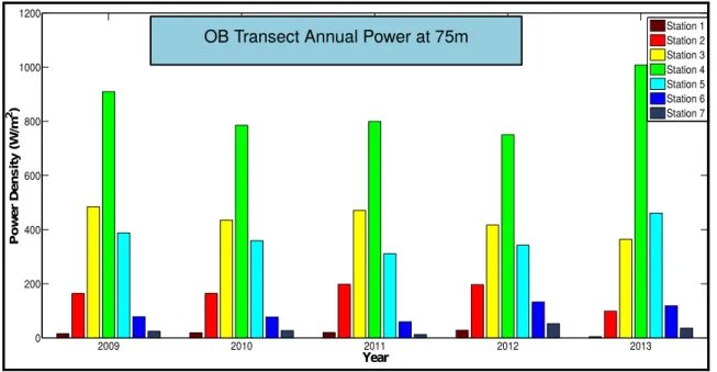
in Onslow Bay. Dark red vertical bars represent station 1, yellow is station 3, green is

station 4, light blue is station 5, dark blue is station 6, and grey is station 7. The

maximum power obtained at the OB transect is 1,008 W m-2_{at station 4 in 2013.}

4.5 Current Roses

Current roses for the 150 kHz ADCP and model were constructed using data from

a depth of 75 m from August 1, 2013 to April 28, 2014. These are shown in Figures 13

and 14 with 0.5 m s-1_{speed bins and 15° directional bins. The speed bins are displayed}

by the following colors: the 0 – 0.5 m s-1_{bin is navy, the 0.5 – 1.0 m s}-1_{bin is dark blue,}

the 1.0 – 1.5 m s-1_{bin is light blue, the 1.5 – 2.0 m s}-1_{bin is green, and the 2.0 – 2.5 m s}-1

bin is yellow. The bearings of the current in both roses lay primarily in quadrant I with

only some bearing of minimal speed in quadrant III. Essentially none of the current

directionality falls in quadrants II and IV for the ADCP and for the model. Dotted radials

in the current roses reference the percentage of the data that falls among the radials. For

the ADCP current rose, the radials are labeled as 20%, 40%, and 60%, and for the model

current rose the radials are labeled as 25%, 50%, and 75%.

4.6 Model vs. ADCP Best-Fit Line

Model speeds were compared against the observed speeds to see if a relationship

could be found among the speed values of the two data sets. These observed speeds are

not the 36-hour low passed speeds, but are hourly interpolated to comply with the

(20)

the ADCP speeds with each circle representing an individual data point. The black line

drawn is the one-to-one line independent of the data, while the other colored lines are

linear, quadratic, and cubic best-fit representations of the relationship between model and

ADCP speeds. The linear fit is light blue, the quadratic curve is magenta, and the cubic

(21)

Section 5: DISCUSSION

5.1 Cross-Isobath Average Current Velocities

Along the North Carolina coastline, the inshore edge of the Gulf Stream is

bounded roughly by the 100 m isobath while the offshore edge of the Stream remains

close to the 4m000 m isobath, such as depicted in Figures 1 and 3. Near the center of

each transect, velocity vectors are slightly greater than 1 m s-1_{(Figure 3). In Figure 3}

there are greater velocities in the center of the transects, which are approximately the

center of the Stream. These speeds diminish moving towards the outer edges of each

transect, which is also towards the edge of the Stream, thus representative of the cyclonic

and anticyclonic shear zones. Comparing the flow regime among the three transects,

Onslow Bay shows more lateral symmetry in the profile.

5.2 Speed and Power Time series

Figure 5 shows how the model compares to the ADCP in speed. The model and

ADCP undergo similar long-term behaviors at lower frequencies. This provides evidence

that the model and ADCP agree well at lower frequencies. This agreement between the

model and ADCP speeds along with the model’s capture of the jet-like structure of the

Gulf Stream is validation for using the model at other offshore sites off of North

Carolina. Inspection of Figure 5 shows stronger agreement of the two signals at lower

frequencies but weaker agreement at higher frequencies. Thus, the model does not seem

to capture the same daily fluctuations as the ADCP but it does capture the bimonthly

fluctuations. While this time series does not cover the span of a whole year, there is

oscillatory behavior at periods longer than bimonthly. It is seen that speed variations

(22)

in speeds are partly due to a slight increase or decrease in the core of the Gulf Stream, but

these changes are mostly due to a lateral shift in the core of the Gulf Stream. For

example, at time scales of several days to a few weeks, meanders cause a lateral shift in

the Gulf Stream that affects the offshore position of the jet. This meandering affects

which of the jet’s isotachs lie over the ADCP location as well as the vertical shear there.

The power time series of Figure 6 is similar to the speed time series in its

oscillatory behavior, but the amplitude and signal differences are far greater. While the

model and ADCP have an exact speed average at 75 m, the power density average for the

two data sets differs by approximately 20%. Since the power is proportional to speed

cubed, more pronounced differences in speed (where the ADCP reaches higher

amplitudes than the model) at times such as August 1, 2013 through mid-October are

cubed thus small speed differences become more discernable in the power density. In

November when the speeds, and hence power, decrease to almost nothing, this suggests

that the Gulf Stream position is farther offshore and the ADCP location is no longer

within the jet. When the speeds get to be this low, the jet maintains its structure but

moves eastward.

Kabir et al., 2015 used HYCOM and a grid at 34.85° N to 35.15°N and 74.85°W

to 74.5°W to find that more than 50% of the days from November 2003 through

December 2012 at 20 m depth exhibit a power density of 500 W m-2_{or greater. This}

overlaps with the offshore end of the CH transect near station 14. Our study concludes

that approximately 48% of the time both the model and ADCP yield power densities

greater than or equal to 500 W m-2_{. This study and}_{Kabir et al}_{., 2015 use different}

(23)

than or equal to 500 W m-2_{. The small difference between the two percentages is likely}

due to the grid’s location being farther offshore than the ADCP site, enabling the grid to

capture more of the core of the current with faster speeds, as well as using different

depths for the studies.

Current wind studies in North Carolina have quantified winds to produce an

average power of 800 W m-2_{. This is very close to the ADCP power density average of}

798 W m-2_{. This suggests that Gulf Stream subsurface turbines may become viable as}

turbine and mooring technology develop.

5.3 Annual Power at Stations

Figure 7 of the model’s annual power at the ADCP location in 2010 has

interesting and unexpected results. The 2010 annual-average of 14 W m-2_{is very low}

compared to the subsequent years, and is 3% of the five-year average and only 1% of the

power in 2012. Meanwhile, the average power in 2012 is 230% of the overall average.

An explanation for these events is an offshore shift of the core of the Stream. In 2010 the

core has shifted offshore so that our location is near the edges of the jet and thus seeing

minimal speeds. Two years later the Stream has shifted onshore and is positioned against

the continental shelf break with the core of the current over the ADCP site and hence

greater speeds. For both of these years it appears the current has had a large horizontal

shift and continues to stay in that shifted position, rather than returning to its previous

state. It would be interesting to see how commonly events like 2010 and 2012 occur on a

longer time span. The other three years, 2009, 2011, and 2013, have averages close to

the five-year average. This is likely a result of the Gulf Stream’s path staying over the

(24)

The station in the CL transect shares similarities in power trends with the ADCP

location in the CH transect but also undergoes some differences. The CL and CH stations

show the same general trend in power averages over the five years. Such that, there are

decreases in power density from 2009 to 2010 and from 2012 to 2013, with increases in

the density from 2010 to 2012 (Figure 8). However, the annual power density values

differ for the CH and CL stations, and the magnitude of the change in power density

differs between each year. The CL station does not contain the same events in 2010 and

2012 as does the CH station, and has a five-year average that is almost 60 W m-2_{less than}

the CH five-year average. For the CH and CL stations, averaging the 2011 and 2012

power averages yields a greater value than averaging the 2009 and 2010 power averages.

Contrary to the findings in the CH station, the OB station did not show significant

variations in power levels for any of the five years, and the five-year average is about a

third of the five-year average at the CH station (Figure 9). Given this lower power, it is

likely that the station in the OB transect spends less time in the core of the current than

the CH station and tends to experience lower current speeds. It is possible that there may

be more offshore and onshore shifts in the Stream in Onslow Bay, but these path shifts

occur more equally distributed along the transect. The annual-averages are much

smoother across the five years, with 2009 and 2010 having very similar power averages

and 2011 and 2012 observing very similar power averages. The average of the 2011 and

2012 annual power averages are greater than the average of the 2009 and 2010 annual

power averages. Moving north to south in our selected stations from each transect, it is

observed that there exists greater power yet more variation in the CH station, with power

(25)

5.4 Annual Power at Transects

Computing the annual power for certain stations in each transect over 2009 –

2013 provides not only temporal coverage but greater spatial coverage by analyzing what

the Gulf Stream is doing at other parts of the transect rather than just at one point. In

2009 at the CH transect there is small lateral variation among the five stations (stations 3,

13, 14, 15, and 16) shown in Figure 10. Greater lateral variation is observed in the

subsequent four years, and with the greatest annual power average reported in station 13

(yellow bar) for all but one year. In 2011- 2013 the power density peaks are greater and

more pronounced, while stations not within the peaks experience much smaller power,

hence greater shearing of the current. Comparing our ADCP location in 2010 to the other

stations in the transect, we see that the station is on the edge of the inshore, cyclonic side

of the Stream, since the greater power is found at the more offshore stations. In 2012 we

again see that the Gulf Stream has shifted onshore, as indicated by the skewed envelope

of the annual-averages. This addresses why the ADCP location experienced such high

power. These lateral movements in the Stream are more easily observed in Figure 10,

allowing easier inspection of the spatial changes in the Stream for comparison.

The addition of the CL and OB transects provide enhanced spatial coverage along

the coast of North Carolina. The horizontal distribution of power is also visible in the CL

transect. The distribution is skewed more to the left with a longer tail on the right. The

power peak for each year fluctuates between stations 5 and 6 (yellow and green bars).

These stations both have a five-year average of roughly 875 W m-2_{, and lie over depths of}

approximately 500 m and 2800 m. This may be important to note when considering the

(26)

of 2,800 m provides a greater challenge for capturing and relaying Gulf Stream power

back to shore. Similar to Figure 9 which shows the annual power of station 2 in Onslow

Bay, the annual OB transect power is more uniform and consistent throughout the five

years. The lateral shear is easily distinguishable, and the greatest power is at station 4

every year. Station 4 has a depth of 654 m, which would be very challenging for

engineering. For four of the five years, station 3 shows the second greatest power.

Station 3, whose five-year average is about 400 W m-2_{, is situated over a depth of 334 m,}

about 100 m deeper than the ADCP location. This is much shallower than the depths of

stations 5 and 6 in the CL transect, and based on its consistent power density over these

five years, it may be a potential subsurface turbine mooring location.

5.5 Current Roses

The current roses for the model and ADCP in Figures 13 and 14 relate current

directionality between the two data sets. Almost all of the time for the model and ADCP

the Stream flows northeast. About 70% of the time for the model and about 60% of the

time for the ADCP, the Stream flows at 45°. There are also a small number of bins in

both roses that lie in the quadrant opposite that of the main flow, i.e. in the southwest

direction. These speeds are very small and only occur less than 2% of the time. This

may be explained by the phenomenon when there are frontal filaments or cold core

eddies propagating through the cyclonic edge of the current. The part of the current that

is within the path of the filament or eddy undergoes a change in the direction that is

almost a 180° rotation from that of the rest of the current. These roses show that flow of

the Gulf Stream at the ADCP site is very unidirectional and at about 45°. While there are

(27)

direction that the water flows within the current is mostly consistent. This agrees with

Kabir et al., 2015 who also found current directionality to be very uniform and in the

northeast direction.

5.6 Model vs. ADCP Best-Fit Line

Comparing the best-fit lines of different degrees to the one-to-one line in Figure

15, it is observed that the slopes of the best-fit lines are more gradual and not as steep as

the one-to-one slope. This means that at higher speeds, the ADCP speeds are greater than

the model speeds. The overlapping and minimal difference in slope of the first, second,

and third degree polynomial fits suggest that the simplified linear representation of the

two data sets is sufficient and preferable over higher degree functions. The slope of this

(28)

Section 6: CONCLUSION

The assessment conducted here shows the MHK energy off of North Carolina. A

150 kHz ADCP and ROMS model are analyzed and the theoretical resource of power is

computed for both data sets and compared. At a depth of 75 m over the ADCP location,

the ADCP and model yield the same nine-month speed average of 0.94 m s-1_{, and the}

direction of the current is very uniform, at about 45°. The power density time series

shows that the ADCP reaches 4,500 W m-2_{with an average of nearly 800 W m}-2_{, making}

it comparable to recent wind studies off of North Carolina. Five-year averages of the

power density for the model range between 150 and 475 W m-2_._{Yang et al}_{., 2014 defines}

the recoverable resource as the amount that can be extracted within current technological

limits. Given the uncertainty in the turbine technology and engineering capabilities, it is

difficult to produce an exact determination of the recoverable resource from the Gulf

Stream. Once known, such parameters can be factored in to the theoretical power density

formula to yield a closer approximation to the recoverable resource, and thus the amount

of Gulf Stream MHK energy that can be supplied for electricity.

A second 150 kHz ADCP was deployed in April 2014 for nine months at the

same location as the first. The data from this ADCP are currently being processed and

will extend the temporal coverage for which there are observational measurements.

Near-future work will consist of comparing this newer data set to the model. Lastly, the

first ADCP was refurbished and deployed in January 2015, and will hopefully provide

another nine months of observations for comparison. The continuation of this study in

understanding the Gulf Stream power characteristics off North Carolina is crucial for the

(29)

the environment. Knowing the resource and environment help lay the foundation for

extracting current energy and therefore must be understood well enough to plan

accordingly.

As society continues to exploit fossil fuels and nonrenewable resources, these

resources will diminish below society’s demands and ultimately we will need to

transition to other resources. In reaching the goal of 80% of US electricity generation

from renewable energy resources by 2050, ocean energy can be an additional resource if

further research is executed along with advances in turbines, mooring technology, and

(30)

REFERENCES

Augustine, C.; Bain, R.; Chapman, J.; Denholm, P.; Drury, E.; Hall, D. G.; Lantz, E.; Margolis, R.; Thresher, R.; Sandor, D.; Bishop, N. A.; Brown, S. R.; Cada, G. F.; Felker, F.; Fernandez, S. J.; Goodrich, A. C.; Hagerman, G.; Heath, G.; O’Neil, S.; Paquette, J.; Tegen, S.; Young, K. (2012), Renewable Electricity Generation and Storage Technologies, Vol 2. of Renewable Electricity Futures Study, NREL/ TP-6A20-54209-2, Golden, CO: National Renewable Energy Laboratory.

Bane, J. M., Brooks, D. A., and Lorenson, K. R. (1981), Synoptic observations of the three-dimensional structure and propagation of Gulf Stream meanders along the Carolina continental margin, J. Geopys. Res., 86, 6411-6425.

Brooks, D. A. and Bane, J. M. (1978), Gulf Stream deflection by a bottom feature off Charleston, South Carolina, Science, 201, 1225-1226.

Brooks, D. A. and Bane, J. M. (1981), Gulf Stream fluctuations and meanders over the Onslow Bay upper continental slope, J. Phys. Oceanogr., 11, 247-256.

Gong, Y., He, R., Gawarkiewicz, G. G., and Savidge, D. K. (2015), Numerical

investigation of coastal circulation dynamics near Cape Hatteras, North Carolina, in January 2005, Ocean Dynamics, 65, 1-15.

Gorban, A. N., Gorlov, A. M., and Silantyev, V. M. (2001), Limits of the turbine

efficiency for free fluid flow, Journal of Energy Resources Technology, 123, 311-317.

Guney, M. S. (2011), Evaluation and measures to increase performance coefficient of hydrokinetic turbines, Renewable and Sustainable Energy Reviews, 15, 3669-3675.

Halkin, D. and Rossby, T. (1985), The structure and transport of the Gulf Stream at 73° W, J. Phys. Oceanogr., 15, 1439-1452.

Hanson, H. P. (2014), Gulf Stream energy resources: North Atlantic flow volume increases create more power, Ocean Engineering, 87, 78-83.

Hanson, H. P., Bozek, A., and Duerr, A. (2011), The Florida current: A clean but challenging energy resource, Eos Trans. AGU, 92, 29-30.

Kabir, A., Lemongo-Tchamba, I., and Fernandez, A. (2015), An assessment of available ocean current hydrokinetic energy near the North Carolina shore,

(31)

Legeckis, R. V. (1979), Satellite observations of the influence of bottom

topography on the seaward deflection of the Gulf Stream off Charleston, South Carolina, J. Phys. Oceanogr., 9, 483–497.

Lissaman, P. B. S. and Radkey, R. L. (1979), Coriolis program: a review of the status of the ocean turbine energy system, Oceans ‘79, 559-565.

Quattrocchi, G.. Pierini, S., and Dijkstra, H. A. (2012), Intrinsic low-frequency

variability of the Gulf Stream, Nonlinear Processes in Geophysics, 19, 155-164.

Shchepetkin, A. F. and McWilliams, J. C. (2005), The regional ocean modeling system (ROMS): a split-explicit, free-surface, topography-following-coordinate oceanic model, Ocean Modelling, 9, 347-404.

Stewart, H. B. (1974), Current from the current, Oceanus, 17, 38-41.

Tracy, K. L. and Watts, D. R. (1986), On Gulf Stream meander characteristics near Cape Hatteras, J. Geophys. Res., 91, 7587-7602.

Yang, X., Haas, K. A., and Fritz, H. M. (2013), Theoretical assessment of ocean Current energy potential for the Gulf Stream system, Marine Technology Society Journal, 47, 1-12.

(32)

Gul f St

ream

“Snapshot” of The

Gulf Stream

March 2008 Longitude L at it u d e Cape Hatteras Cape Lookout clouds

Sea Surface Temperature

Cape Fear

Close

Appr_oach

to Ca_{pe H}

a eras Close Appro ach toSE Florid a 100m

Figure 1. A sea surface temperature (SST) snapshot of the Gulf Stream along the US

(33)

Gulf Stream Current Speed

m/sec Shelfbreak

Coastline

SST Front

30km 80-150 km

WIND TURBINES

GULF STREAM TURBINES

0.4 0.6

0.8 1.0 1.2 1.4

(34)

Figure 3. 2013 average current velocities at 75 m overlying a North Carolina base map. Stations in the cross-isobath transects are shown by yellow circles with both model and observational data at the blue circle. The transects are labeled CH for Cape Hatteras, CL for Cape Lookout, and OB for Onslow Bay. Green arrows show the current velocity. Isobaths are the black contour lines with the 100 m isobath in bold. The four blue stars show the locations of the cities Virginia Beach, Kitty Hawk, Morehead City, and Wilmington. These are sites to connect MHK energy from the Gulf Stream to the power grid.

Onshore Grid Connections

Onshore Grid

Connections

Virginia Beach

Kitty Hawk

Morehead City

Wilmington

ADCP

OB

CL

(35)

(36)

October January April 0 0.5 1 1.5 2 2.5 Months S p ee d ( m /s ) Model ADCP Model Average = .94 m/s

ADCP Average = .94 m/s

Figure 5. Time series of the current speed at 75 m from August 1, 2013 thru April 28,

2014. Model speeds are shown in red and ADCP speeds in blue. The horizontal black bar is the model and ADCP average speed of 0.94 m s-1_.

October January April

0 500 1000 1500 2000 2500 3000 3500 4000 4500 Months P o w e r (W /m 2 ) Model ADCP

Model Average = 641 W/m2

ADCP Average = 798 W/m2

Figure 6. Time series of the power density at 75 m from August 1, 2013 thru April 28,

2014. Model time series is shown in red and ADCP time series in blue. The red horizontal bar shows the model power density average of 641 W m-2_{, and the blue}

horizontal bar shows the ADCP power density average of 798 W m-2_.

Current Speed 8/1/13 – 4/28/14 at 75m

(37)

2009 2010 2011 2012 2013 0

100 300 500 700 900 1,100

Year

P

o

w

e

r

D

e

n

s

it

y

(

W

/m

(38)

Figure 7. Five-year model annual power density averages from 2009 – 2013 at 75 m at station 3 (ADCP location) in the Cape Hatteras transect. The horizontal dashed line is the five-year average of 467 W m-2_.

2009 2010 2011 2012 2013

0 100 300 500 700 900 1,100 Year P o w e r D e n s it y ( W /m 2 )

station 3 in the Cape Lookout transect. The horizontal dashed line is the five-year average of 402 W m-2_.

Annual Power CH Station 2 at 75m

(39)

2009 2010 2011 2012 2013 0

100 300 500 700 900 1,100

Year

P

o

w

e

r

D

e

n

s

it

y

(

W

/m

2 )

station 2 in Onslow Bay transect. The horizontal dashed line is the five-year average of 164 W m-2_.

(40)

2009 2010 2011 2012 2013 0 200 400 600 800 1000 1200 Year P o w er D en si ty ( W /m 2 ) Station 3 Station 13 Station 14 Station 15 Station 16

multiple stations in the Cape Hatteras transect. Red vertical bars of station 3 (ADCP location) are the same as those in Figure 7. These are the same stations in the Cape Hatteras transect with average current velocities in Figure 3.

2009 2010 2011 2012 2013

0 200 400 600 800 1000 1200 Year P o w er D en si ty ( W /m 2 ) Station 3 Station 5 Station 6 Station 7 Station 8 Station 9 Station 10

multiple stations in the Cape Lookout transect. Red vertical bars of station 3 are the same as those in Figure 8. These are the same stations in the Cape Lookout transect with average current velocities in Figure 3.

CH Transect Annual Power at 75m

(41)

2009 2010 2011 2012 2013 0 200 400 600 800 1000 1200 Year P o w e r D e n s it y ( W /m 2) Station 1 Station 2 Station 3 Station 4 Station 5 Station 6 Station 7

multiple stations in the Onslow Bay transect. Red vertical bars of station 2 are the same as those in Figure 9. These are the same stations in the Onslow Bay transect with average current velocities in Figure 3.

(42)

Figure 13. ADCP current rose from August 1, 2013 thru April 28, 2014 at 75 m. Percentages show the time spent in a given direction.

Figure 14. Model current rose from August 1, 2013 thru April 28, 2014 at 75 m.

Percentages show the time spent in a given direction.

8/1/13 – 4/28/14 Current Rose for 150 kHz ADCP at 75m

(43)

0 0.5 1 1.5 2 0

0.5 1 1.5 2

ADCP Speeds (m/s)

M

od

el

S

pe

ed

s

(m

/s

(44)

Figure 15. Model speeds vs. ADCP speeds from August 1, 2013 thru April 28, 2014 at 75 m. The black line shows the one-to-one line. The linear fit is shown by the light blue line, the quadratic line is represented by the magenta curve, and the cubic fit is displayed by the red curve.

(45)

Table 1. Cape Hatteras Cross-Isobath Transect Stations

Cape Hatteras

Station Latitude (°) Longitude (°) Depth (m)

CH 1 35.18 -75.17 62

CH 2 35.16 -75.13 102

CH 3 35.14 -75.11 222

CH 4 35.13 -75.10 271

CH 5 35.14 -75.09 315

CH 6 35.12 -75.08 376

CH 7 35.12 -75.07 460

CH 8 35.11 -75.06 614

CH 9 35.11 -75.05 695

CH 10 35.10 -75.05 884

CH 11 35.10 -75.04 1058

CH 12 35.09 -75.03 1265

CH 13 34.97 -74.83 2779

CH 14 34.85 -74.63 3107

CH 15 34.73 -74.43 3276

CH 16 34.61 -74.23 3548

Table 2. Cape Lookout Cross-Isobath Transect Stations

Cape Lookout

CL 1 34.44 -76.00 53

CL 2 34.40 -75.95 80

CL 3 34.36 -75.90 174

CL 4 34.32 -75.85 268

CL 5 34.27 -75.80 488

CL 6 34.11 -75.60 2775

CL 7 33.94 -75.40 3031

CL 8 33.78 -75.20 3316

CL 9 33.61 -75.00 3617

(46)

Table 3. Onslow Bay Cross-Isobath Transect Stations

Onslow Bay

OB 1 33.57 -76.90 96

OB 2 33.48 -76.80 212

OB 3 33.40 -76.70 374

OB 4 33.23 -76.50 654

OB 5 33.07 -76.30 1076

OB 6 32.90 -76.10 2147

(47)

APPENDIX

Raleigh Bay

RB 1 34.75 -75.60 84

RB 2 34.69 -75.47 356

RB 3 34.58 -75.26 2647

RB 4 34.46 -75.03 3013

RB 5 34.40 -74.90 3167

(48)

Figure A. 2013 average current velocity at a depth of 28 m for the CH, RB, CL, and OB transects. Green arrows show the average velocity from the model at each of the stations (yellow circles).

8/1/13-4/28/14 Average Vector Velocity 28m

CH

RB

CL

(49)

Figure B. Current speed time series for the model and ADCP at 28 m from August 1, 2013 through April 28, 2014. The model is the green time series and the ADCP is the blue time series. The black line shows the model and ADCP average speed, which are too close together to distinguish.

Figure C. Betz power time series for the model and ADCP at 28 m for August 1, 2013

through April 28, 2014. The model is the green time series and the ADCP is the blue time series. The green line shows the model average of 5.32 MW (1149 W m-2_{) and the}

blue line shows the ADCP average of 6.5 MW (1403 W m-2_).

8/1/13 – 4/28/14 Current Speed of Model & ADCP 28 m

(50)

Figure D. Average current velocities for the model and ADCP at 28 m from August 1, 2013 through April 28, 2014. The green arrow shows the model average and blue arrow shows the ADCP average.

8/1/13-4/28/14 Average Vector Velocity Model &

(51)

Figure E. ADCP current rose from August 1, 2013 thru April 28, 2014 at 28 m. Percentages show the time spent in a given direction.