Sharif University of Technology
Scientia IranicaTransactions B: Mechanical Engineering www.scientiairanica.com
Synthesis of robust PID controller for controlling a
single input single output system using quantitative
feedback theory technique
M.R. Gharib
and M. Moavenian
Department of Mechanical Engineering, Ferdowsi University of Mashhad, Mashhad, Iran. Received 27 December 2011; received in revised form 22 January 2014; accepted 17 March 2014
KEYWORDS Quantitative Feedback Theory (QFT); Rotary missile; Nonlinear equations; Robust PID.
Abstract. In this paper, the modeling and control of a rotary missile that uses the proportional navigation law is proposed, applying the Quantitative Feedback Theory (QFT) technique. The dynamics of a missile are highly uncertain; thus, application of robust control methods for high precise control of missiles is inevitable. In the modeling section, a new coordinate system has been introduced, which simplies analysis of rotary missile dynamics equations. In the controlling part, application of the QFT method leads to the design of a robust PID controller for the highly uncertain dynamics of a missile. Since missile dynamics have multivariable nonlinear transfer functions, in order to apply the QFT technique, these functions are converted to a family of linear time invariant processes with uncertainty. Next, in the loop shaping phase, an optimal robust PID controller for the linear process is designed. Lastly, analysis of the design procedure shows that the robust PID controller is superior to the commonly used PID scheme and multiple sliding surface schemes, in terms of both tracking accuracy and robustness.
© 2014 Sharif University of Technology. All rights reserved.
1. Introduction
Closed loop controlled missiles are designed, taking into consideration that they do not rotate around the longitudinal axis [1-8]. In order to control these missiles, we must control yaw and pitch channels independently. For analyzing the dynamics of a mis-sile, both earth-xed and body coordinate systems are normally employed. But, in this paper, a new coordinate system has been introduced which results in simplication of the dynamic modeling analysis, and obtains a linear uncertain SISO dynamic model for the missile. The main dierence between con-trolling a Multiple-Input Multiple-Output (MIMO) system and a Single-Input Single-Output (SISO)
sys-*. Corresponding author. Tel.: +98 915 322 8499
E-mail address: Mech [email protected] (M.R. Gharib)
tem is in the process of assessing and compensat-ing the interactions in the system degrees of free-dom [9,10].
In summary, one can say that it is a complicated issue to implement an established SISO system control model on a MIMO system, because of extensive com-putational load.
The advantage of QFT, with respect to other robust control techniques such as H1 [11-16], is that
their design is based on the magnitude of transfer function in the frequency domain. However, design of QFT [17-26] is not only concerned with the aforemen-tioned subject, but is also able to take into account phase information. The unique feature of QFT is that the performance specications are expressed as bounds on frequency-response loop shapes in such a way that the satisfaction of these bounds implies a corresponding approximate closed-loop satisfaction
Figure 1. Two-degree-of-freedom feedback system.
of time-domain response bounds for given classes of inputs and for all uncertainty in a given compact set.
Consider the feedback system shown in diagram of Figure 1. This system has a two-degree-of-freedom structure. In this diagram, p(s) is an uncertain plant belonging to a set that is p(s) 2 fp(s; ); 2 pg, where is the vector of uncertain parameters. P (s) and G(s) are plants with an uncertainty structure and a xed structure feedback controller, respectively. F (s) is the pre-lter and D(s) is the disturbance at the plant output.
2. Missile's model
To obtain the missile's dynamic model, three coordi-nate systems are dened.
The origin of the earth-xed coordinate system is located at the missile's launch point [1,3].
The origin of the body coordinate system is assumed to be at the missile center of gravity. The XB-axis of the body coordinate system points in the
direction of the missile nose, the YB-axis points in
the starboard direction, and the ZB-axis completes the
right-handed triad [3].
A new method for dynamic modeling of a rotary missile, based on suggesting a new irrotational body coordinate system, has been introduced, which elimi-nates the interaction between pitch and yaw channels. This coordinates system is dened as below:
The body irrotational coordinates system is as-sumed to be at the missile's center of gravity. The XS-axis system points in the direction of the missile
nose, the YS-axis in the yaw channel, and the ZS-axis
in the pitch channel.
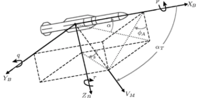
The body coordinate system and the inertial coordinate systems are used to derive the equations of motion. These coordinate systems are illustrated in Figure 2.
Based on Newton's second rule, we know that the force is equal to changes in the vector of momen-tum [1]:
F = FS =F
X FY FZT; (1)
! = !S IS =
p q rT; (2) V = Vs=u v wT; (3)
Figure 2. Missile's coordinate systems [3].
8 > > > < > > > :
Fx= _Mu + M( _u + qw rv)
Fy= _Mv + M( _v + ru pw)
Fz= _Mw + M( _w + pv qu)
(4)
where u, v and w are the speed components measured in the missile body axes system, and p, q and r are the components of the body angular velocity [1,3].
Consider that HS = I!S
IB and I is the moment
of inertia of the missile in the body irrotational coordi-nates system. By reason of symmetry around the mis-sile longitudinal axis, I matrix is I = diagfIxx; IzzIzzg.
Also, !S
IB is the angular velocity vector (that rotates
with the body coordinate system), which is expressed in terms of frame fSg.
If the angular velocity around the longitudinal axis is s, then:
!S
IB = !SIS+
s 0 0T =s + p q rT: (5) So, by applying Eq. (5) and the denition of HS:
HS = I!S IB =
Ixxp + Ixxs Izzq Izzr: (6)
Using Eq. (6), Coriolis and Newton's rules, and assum-ing 2=l m nT (where is a vector of moment),
yields [1]: 8 > > > < > > > :
l = _Ixx(p + s) + Ixx( _p + _s)
m = _Ixxq + Izz_q + (Ixx Izz)qr + Ixxsr
n = _Ixxr + Izz_r (Izz Ixx)pq Ixxsq
(7)
2.1. Linearization of model The state vector is dened as [1,5]:
x =u v w p q rT:
Angle of attack () and angle of sideslip () can be dened as follows:
= tan 1 v
u
; = tan 1w
u
Figure 3. Motion variable notations.
Aerodynamics force and moment are functions of the angles of attack (), sideslip, ns (p; d) and angular velocity (p; q; r) (Figure 3) [1].
Since the missile has one movable n, as a result of rotation, it can be supposed that the missile has two movable ns, separately, in y, z directions in the body irrotational coordinate system.
The equivalent n in the Y -axis direction is named the lifter n, and p is a small deviation of it. The second n is named the rotating n and d is a small deviation of that.
For linearization, aerodynamics force and moment are assumed linear functions.
The translational and rotational dynamics of the missile are described by the following six nonlinear dierential equations:
_x1=
_ M0=M0
x1 x2x6 x3x5
+ (1=M0)
n
tan 1(x
3=x1)Cx
+ tan 1(x
2=x1)Cx+ Cxpp + Cxdd
+ Cyqx5+ Fxprop ;
_x2=
_ M0=M0
x2 x1x6 x3x4
+ (1=M0)tan 1(x3=x1)Cy
+ tan 1(x
2=x1)Cy+ Cypp + Cydd
+ Cyqx5+ Fyprop ;
_x3=
_ M0=M0
x3 x1x5 x2x4
+ (1=M0)tan 1(x3=x1)Cz
+ tan 1(x
3=x1)Cz+ Czpp
+ Czdd + Czqx5+ Fzprop ;
_x4= _Ixx0=Ixx0x4 _Ixx0=Ixx0s
+ (1=Ixx0)tan 1(x3=x1)Cl+ Clpp
+ Cldd + Clpx4+ lprop ;
_x5=
_Izz0=Izz0
x5+ I0x4x6 (Ixx0s=Izz0)x6
+ (1=Izz0)tan 1(x3=x1)Cm
+ tan 1(x
2=x1)Cm+ Cmpp + Cmdd
+ Cmrx5+ mprop ;
_x6=
_Izz0=Izz0
x6+ I0x4x5 (Ixx0s=Izz0)x5
+ (1=Izz0)tan 1(x3=x1)Cn
+ tan 1(x
2=x1)Cn+ Cnpp + Cndd
+ Cnrx6+ nprop ; (9)
where I0= (Izz0 Ixx0)=Izz0and prop index are related
to forces and moments produced from combustion of the missile, and C coecients are aerodynamic factors of the missile. The result of linearizing Eq. (9) in the operating point (V0; !0), when u = u0+ u, is given
by [4], as follows:
X = 2 6 6 6 6 6 6 4
A1 A2 A3 0 0 0 0 A4 0 0 0 A5 0 0 A6 0 A7 0 0 0 0 A8 0 0 0 0 A9 0 A10 A11 0 A12 0 0 A13 A14 3 7 7 7 7 7 7 5 X + 2 6 6 6 6 6 6 4 B1 B1 0 B1 B1 0 0 0 B1 0 0 B1 3 7 7 7 7 7 7 5 u; (10)
A1 A2 A3
_ M0
M0 u0M0Cx u0M0Cx
A4 A5 A6
_ M0
M0 +u0M0Cy u0+ Cyr M0M0_ +u0M0Cz
A7 A8 A9
u0+ Czq _Ixx0Ixx0+Clp u0ICmzz0
A10 A11 A12
_Izz0+Cmq Izz0
Ixx0s Izz0
Cn u0Izz0
A13 A14 B1
Ixx0s Izz0
_Izz0+Cnr
Izz0 CXp
According to the state space model, x2 is related
to x6, x3 is related to x5. x2 and x6 states represent
the yaw channel, while x3 and x5 states express the
pitch channel in common missiles. The main system can be divided into two subsystems; yaw and pitch channels. x1 and x4 states have no eect on pitch
and yaw channels, but the stability of these channels causes the stability of x1 and x4 states. The outputs
of the system are the angular velocities of the missile (in the normal direction of the longitudinal axis).These angular velocities are related to pitch and yaw channels. By controlling the missile in these channels, a good performance will be resulted. In the irrotational body coordinate system, the only interaction between these channels is the term (Ixx0s=Izz0). According to the
physical shape of the missile, Izz0 is approximately 100
times greater than Ixx0. By ignoring the interaction
between these channels, the state space of the pitch channel is:
y =0 1 x2
x6 ; _x2 _x6 = 2 6 4 _ M0
M0+u0M0Cy u0+ cyr cn
u0Izz0
_Izz0+cnr Izz0 3 7 5 x2 x6 + cyd cnd d: (11)
From state equations to transfer function. Con-sider the system described by state Eq. (11). The system's transfer function, G(s), is G(s) = C(sI A) 1B + D.
According to the relation between aerodynamic coecients in yaw and pitch channels, in these chan-nels, transfer functions between output (angle of n) and input (angular velocity) are identical and only dier in the sign. So, the designed controller for one channel can be used for another channel by changing its sign.
A missile is a guidable ying machine with vari-able transfer functions. This means that by changing the speed, ying height and mass, and the parameters of ying, the transfer function will change. Variation of speed is especially important, which causes variation in the aerodynamic coecients. So, by applying Eq. (12), shown in Box I, and using a servo motor at four dierent Machspeeds, the missile transfer functions will be obtained.
For the model of the pitch channel missile:
P (s) = cs3+ dsas + b2+ es + 1;
a =0:27 1:7; b =0:41 1:7; c =1:4 10 6 1:47 10 5;
d =0:0016 0:0073; e =0:31 0:91: (13)
3. Quantitative Feedback Theory (QFT) There are many practical systems that have high un-certainty in open-loop transfer functions, which makes it very dicult to have suitable stability margins and proper performance in command following problems in the closed-loop system. Therefore, a single xed controller in such systems is found amongst the \robust control" family.
Quantitative Feedback Theory (QFT) is a robust feedback control-system design technique initially in-troduced by Horowitz (1963, 1979), which allows direct design to closed-loop robust performance and stability specications. Since then, this technique has been further developed by him and others [9-21].
Simply, the QFT controller design method can be summarized as follows.
In parametric uncertain systems, we must rst generate plant templates prior to the QFT design (at a xed frequency, the plant's frequency response set is called a template). Given the plant templates, QFT converts closed loop magnitude specications into magnitude constraints on a nominal open-loop function (these are called QFT bounds). A nominal open loop function is then designed to simultaneously satisfy its constraints, as well as to achieve nominal closed loop stability. In a two-degree-of-freedom design, a pre-lter will be designed after the loop is closed (i.e., after the controller has been designed) [12].
4. Optimal controller design
QFT tunes the G controller with the objective of reducing control bandwidth while maintaining robust performance. A desired modication in small frequency bands is transparent using QFT's open-loop tuning. The bandwidth control point of view was introduced
r d=
Cnds +
C nd _M0
M0 +
CnCyd
u0Izzo
CndCy
u0M0 s2+M_0
M0
Cy
u0M0 +
_Izzo
Izzo
Cnr
Izzo
s +M_0_Izzo
M0Izzo +
CyCnr
u0MoIzzo
Cy_Izzo
u0MoIzzo
_ M0Cnr
M0Izzo +
Cn
Izzo
CnCyr
u0Izzo
: (12)
by Chait and Hollot (1990) [22-26]. A key limitation of the mentioned procedure is that the poles of T are xed with only the zeros taken as optimization variables. So, in the second step, we optimize the denominator coecients, where the cost function is the quadratic sum of Euclidean distance between the open-loop response and the bounds in the Nichols plane. This minimization tries to reach the optimal loop-shaping dened by Zhang et al. [27] and Horowitz and Sidi [31].
In the design stage (loop-shaping), the controller, GC(s), is synthesized by adding poles and zeros until
the nominal loop, dened as L0= G0GC, lies near its
bounds. An optimal controller will be obtained if it meets its bounds while it has minimum high frequency gain. So, application of this method to obtain the min-imum gain of the controller is employed here. Hence, there is no need to be concerned about saturation. As a comprehensive optimal QFT controller design is not the main contribution of this paper, it will be dealt with in future research.
5. PID controller
A realistic denition of optimum in LTI systems is min-imization of the high-frequency loop gain, k, while sat-isfying performance bounds. This gain aects the high-frequency response, since lim
!!1[L(j!)] = K(j!) ,
where is the excess of poles over zeros assigned to L(j!). Thus, only the gain, K, has a signicant eect on the high-frequency response, and the eect of the other parameter uncertainty is negligible. It has been shown that if the optimum, L0(j!) exists, then, it
lies on the performance bounds at all !i, and it is
unique [14]. In this part, we will introduce a simple algorithm for designing an optimal PID controller. A PID controller has a transfer function;
Gpid(s) = kp+ksi + kds: (14)
Three used terms in Eq. (14) are dened as: kp
(propor-tional gain), ki(integral gain) and kd(derivative gain).
Our method for designing an optimal PID controller is based on designing a specic lead-lag compensator, which transforms into a PID controller under special conditions.
Consider the closed-loop system in Figure 1 in which G(s) is a below lag-lead compensator:
G(s) = Ka s +
1 T1
s + a
T1
s + 1 T2
s + 1 aT2
: (15)
In order to achieve a PID controller, let us move a towards innity value, so, we will have:
lim
a!1G(s) =
KT1
s
s +T1
1
s +T1
2
; (16)
) G(s) = KT1
1 T1+
1 T2
+
K T2
1
s+KT1s:(17)
So, we have a PID controller which is dened by:
kp= K
T1+ T2
T2
; ki= TK
2; kd= KT1(18):
Up to now, two real poles of the lag-lead compensator have been specied: one located in innity and the other in the origin. In order to dene the PID controller in the next step of this algorithm, we must specify the gain, K, and the situation of two zeros of G(s). But, as mentioned before, the optimum, L0(j!), must
lie exactly on its performance bounds at all frequency values (!i). Therefore, in the last phase of this
algorithm, the suitable location of these two zeros can be achieved by a trial and error procedure using the Interactive Design Environment (IDE) of QFT [21].
Under special circumstances, using only one zero in the loop shaping phase will result in the PI con-troller (considering the lag-compensator), and the PD controller will be resulted by elimination of the pole in the origin.
6. Design of robust controller for the missile The objective of this part is to synthesize a suitable controller and pre-lter, such that, rst, the closed loop system is stable and, second, it can track the desired inputs.
1. Stability margin:
1 + P (j!)G(j!)P (j!)G(j!) < 1:2: (19)
2. The tracking specication is overshoot (= 5%) and the settling time (= 0:005 s) for all plant uncertainty, which can be described with a second order system:
j(j!i)j jT (j!i)j j(j!i)j ; (20)
where (j!i) and (j!i) are lower bound and
upper bounds, respectively, and T (j!i) is the
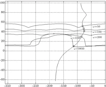
input-output relation from input R(s) to input-output Y (s). At the rst step, the plant uncertainty must be dened (template). Thus, the boundaries of the plant templates have been computed and are shown in Figure 4. Next, having plant templates and required performance specications, we can compute robust performance bounds, which are shown in Figure 5. Then, by having robust performance bounds in the loop-shaping phase of the design, by applying the algorithm developed in part 4, we can design a suitable
Figure 4. Plant uncertainty templates.
Figure 5. Intersection bounds.
PID controller. Figures 6 and 7 depict the loop and prelter shaping of the open loop transfer function. In the loop shaping design, one can observe that the nominal plants lie on their performance bounds, which conrms the optimal design of robust controllers. According to the loop shaping phase, optimal robust PID controllers are as follows:
G(s)PID= 169 + 0:17s +2:15 10 4
s ; (21) F (s) = s
3596+ 1
1 s
4782+ 1 1
: (22)
7. Analysis of design
In this part, the robust stability of the closed-loop system and, also, tracking specications in both time and frequency domains is investigated for all considered uncertainty of the missile dynamics. Frequency domain stability is shown in Figure 8.
Figure 6. Loop shaping of open-loop system.
Figure 7. Prelter shaping of open-loop system.
Figure 8. Robust stability of closed-loop system.
The frequency-domain closed-loop response is shown in Figure 9 and, consequently, the time-domain closed-loop response is shown in Figure 10. Hence, according to linear simulation, the missile has ro-bust stability and can also satisfy tracking specica-tions.
Figure 9. Closed-loop frequency response.
Figure 10. Unit step response.
Figure 11. Tracking performance of pitch angle (t) to the commanded pitch angle d(t) (solid line: d(t), dotted line: (t)) using MSS [32].
7.1. Comparison of QFT controller with MSS control approach in control of pitch channel
Angular tracking responses were used to evaluate the control performance of the missile pitch channel. Fig-ures 11 and 12 show simulations of angular tracking
Figure 12. Tracking performance of pitch angle using QFT.
Figure 13. Tracking errors versus time of pitch angle using MSS [29].
responses related to MSS [32] and QFT applied in this work, respectively.
Comparison of the MSS [32] method with the QFT controller, regarding angular tracking errors, demonstrates that the QFT technique, in the presence of all uncertainties, suggests a controller which has a better control performance, with respect to maximum and integral absolute errors (Figures 13 and 14).
8. Conclusion
In this article, after achieving the dynamic model of the missile, QFT is introduced as a robust controlling design method, and application of the proposed third coordinate system simplied the dynamic modeling of the missile. This caused the nonlinear MIMO system to be converted to a linear SISO system. In order to compensate the uncertainties involved, a family of linear uncertain SISO systems is introduced. Then,
Figure 14. Tracking errors versus time of pitch angle using QFT.
an optimal robust PID controller for the linear process is designed. Finally, the results obtained from the controller output designed using the QFT method are compared with reported results of a multiple sliding surface controller designed by \Lu, Zhao. et al." [32]. It is shown that the QFT technique suggests a controller with a better control performance.
Nomenclature
Angle of attack ()
Angle of sideslip ()
p Small deviation of lift n d Small deviation of rotating n (S) Uncertain parameters vector
!x; !y; !z Angular velocity components (rad/s)
Deection angle in the pitch plane ()
Deection angle in the yaw plane ()
kd Derivative gain
Fractional derivative Fractional integration P (s; ) Uncertain plant Xb; Yb; Zb Body coordinate
G(s) Compensator
Fx; Fy; Fz Components of total forces acting on
missile (N)
Mx; My; Mz Components of total moments acting
on missile (N m) D(s) Disturbance Cx Drag coecient
Xg; Yg; Zg Ground coordinate
ki Integral gain
u; v; w Velocity components (m/s)
S Laplace variable Cz Lateral coecient
Cy Lift coecient
Ix; Iy; Iz Moment of inertia components (kg
m2/s)
F (s) Pre-lter
kp Proportional gain
r Reference signal
M The mass of missile (kg)
References
1. Blacklock, J.H., Automatic Control of Aircraft and Missile, 2nd Ed., John Wiley & Sons Publition, New York, Chaps. 1, 4, 7, 8 (1991).
2. Zarchan, P. \Proportional navigation and weaving targets", Journal of Guidance, Control and Dynamics, 18(5), pp. 969-974 (1995).
3. Menona, P.K. and Ohlmeyer, E.J. \Integrated design of agile missile guidance and autopilot systems", Con-trol Engineering Practice Journal, 9(10), pp. 1095-1106 (2001).
4. Seraj, H. and Masominya, M.A. \Modeling and control of a rotational missile", ICEE Conference, Isfahan, pp. 10- 17, Printed in Farsi (2000).
5. Faruqi, F.A. and Lan Vu, T., Mathematical Models for a Missile Autopilot Design, 1st Ed., DSTO Systems Sciences Laboratory Publication, Edinburgh, South Australia (2002).
6. Lidan, X., Ke'nan, Z., Wanchun, Ch. and Xingliang, Y. \Optimal control and output feedback considerations for missile with blended aero-n and lateral impulsive thrust", Chinese Journal of Aeronautics, 23, pp. 401-408 (2010).
7. Ahmeda, W.M. and Quan, Q. \Robust hybrid control for ballistic missile longitudinal autopilot", Chinese Journal of Aeronautics, 24, pp. 777-788 (2011).
8. Mingzhe, H., Xiaoling, L. and Guangren, D. \Adaptive block dynamic surface control for integrated missile guidance and autopilot", Chinese Journal of Aeronau-tics, 26(3), pp. 741-750 (2013).
9. Gharib, M., Amiri Moghadam, A.A. and Moavenian, M. \Optimal controller design for two arm manipula-tors using quantitative feedback theory method", 24th International Symposium on Automation and Robotics in Construction, India (2007).
10. Yaniv, O. \Automatic loop shaping of MIMO con-trollers satisfying sensitivity specications", ASME Journal of Dynamic Systems, Measurement, and Con-trol, 128, pp. 463-471 (2006).
11. Kim, C.S. and Lee, K.W. \Robust control of robot manipulators using dynamic under parametric uncer-tainty", International Journal of Innovative Compen-sators Computing, Information and Control, 7(7(B)), pp. 4129-4139 (2011).
12. Bi, Sh., Deng, M. and Inoue, A. \Operator based robust stability and tracking performance of MIMO nonlinear systems", International Journal of Innova-tive Computing, Information and Control, 5(10(B)), pp. 3351-3358 (2009).
13. Tootoonchi, A.A., Gharib, M.R. and Farzaneh, Y. \A new approach to control of robot", IEEE RAM, pp. 649-654 (2008).
14. Fateh, M.M. \Robust control of electrical manipulators by joint acceleration", International Journal of Inno-vative Computing, Information and Control, 6(12), pp. 5501-5511 (2010).
15. Moghadam, A., Gharib, M.R., Moavenian, M. and Torabi, K. \Modeling and control of a SCARA robot using quantitative feedback theory", Proc. IMechE Part I: J. Systems and Control Engineering, 223(17), pp. 901-918 (2009).
16. Isidori, A., Nonlinear Control Systems, Berlin, Springer (1989).
17. Horowitz, I.M. \Survey of quantitative feedback the-ory", Int. J. Control Journal, 53(2), pp. 255- 261 (1991).
18. Golubev, B. and Horowitz, I.M. \Plant rational trans-fer function approximation from input-output data", International Journal of Control, 36(4), pp. 711-723 (1982).
19. Jayasuriya, S., Nwokah, O., Chait, Y. and Yaniv, O. \Quantitative feedback (QFT) design: Theory and applications", American Control Conference Tutorial Workshop, Seattle, Washington (June 19-20, 1995).
20. Yaniv, O. and Horowitz, I.M. \Quantitative feedback theory for uncertain MIMO plants", International Journal of Control, 43, pp. 401-421 (1986).
21. Kerr, M.L., Jayasuriya, S. and Asokanthan, S.F. \Ro-bust stability of sequential multi-input multi-output quantitative feedback theory designs", ASME Journal of Dynamic Systems, Measurement, and Control, 127, pp. 250-256 (2005).
22. Zoloas, A.C. and Halikias, G.D. \Optimal design of PID controllers using the QFT method", IEE Proc-Control Theory Appl, 146(6), pp. 585-589 (1999).
23. Lin, T.C., Kuo, M.J. and Hsu, C.H. \Robust adaptive tracking control of multivariable nonlinear systems based on interval type-2 fuzzy approach", Interna-tional Journal of Innovative Computing, Information and Control, 6(3(A)), pp. 941-963 (2010).
24. Garca-Sanz, M., Ega~na, I. and Barreras, M. \De-sign of quantitative feedback theory non-diagonal con-trollers for use in uncertain input multiple-output systems", IEEE Proceedings-Control Theory and Applications, 152(2), pp. 177-187 (2005).
25. Yang, S.H. \An improvement of QFT plant template generation for systems with anely dependent para-metric uncertainties", Journal of the Franklin Insti-tute, 346(7), pp. 663-675 (2009).
26. Wang, Y.F., Wang, D.H., Chai T.Y. and Zhang, Y.M. \Robust adaptive fuzzy tracking control with two errors of uncertain nonlinear systems", International Journal of Innovative Computing, Information and Control, 6(12), pp. 5587-5597 (2010).
27. Zhang, Y., Liang, X., Yang, P., Chen, A. and Yuan, Z. \Modeling and control of nonlinear discrete-time systems based on compound neural networks", Chinese Journal of Chemical Engineering, 17(3), pp. 454-459 (2009).
28. Yanou, A., Deng, M. and I.A. \A design method of extended generalized minimum variance control based on state space approach by using a genetic algorithm", International Journal of Innovative Computing, Infor-mation and Control, 7(7(B)), pp. 4183-4195 (2011).
29. Chait, Y. and Hollot, C.V. \A comparison between H-innity methods and QFT for a SISO plant with both parametric uncertainty and performance speci-cations", O.D.I Nwokah, Ed., Recent Development in Quantitative Feedback Theory, pp. 33-40 (1990).
30. Horowitz, I.M. \Optimum loop transfer function in single-loop minimum-phase feedback systems", Int. J. Control, 1, pp. 97-113 (1973).
31. Horowitz, I.M. and Sidi, M. \Optimum synthesis of non-minimum phase feedback systems with plant un-certainty", Int. J. Control, 27(3), pp. 361-384 (1978).
32. Lu, Zhao, Lin, Feng and Ying, Hao \Multiple sliding surface control for systems in nonlinear block control-lable form", Cybernetics and Systems: An Interna-tional Journal, 36, pp. 513-526 (2005).
Biographies
Mohammad Reza Gharib was born in Mashhad, Iran, in 1981. He received BS and MS degrees in Mechanical Engineering, in 2004 and 2006, from Ferdowsi University of Mashhad, Iran, where he is cur-rently pursuing his PhD degree. His current research interests include control theories, mainly focusing on Quantitative Feedback Theory and the dynamics of quadrotors.
Majid Moavenian received his Bachelor of Science in Mechanical Engineering from the University of Tabriz, Iran. He also earned his MSc and PhD Degrees in Mechanical Engineering from Aston University and University of Wales College Cardi, respectively. Cur-rently he is an associate professor at Ferdowsi Univer-sity of Mashhad while his research interests are in the areas of system design and fault detection.