Project Completion Time in Dynamic
PERT Networks with Generating Projects
A. Azaron 1
and M. Modarres
In this paper, an analytical method is developed to compute the project completion time distribution in a dynamic PERT network, where the activity durations are exponentially distributed random variables. The projects are generated according to a renewal process and share the same facilities. Thus, these projects cannot be analyzed independently. The authors' approach is to transform this dynamic PERT network into a stochastic network and, then, to obtain the project completion time distribution by constructing a proper continuous-time Markov chain. This dynamic PERT network is represented as a network of queues, where the service times represent the durations of the corresponding activities and the arrival stream to each node follows a renewal process. Finally, the proposed methodology is extended to the generalized Erlang activity durations.
INTRODUCTION
Although project scheduling and management have been investigated by many researchers, one cannot nd many models regarding dynamic project scheduling in the literature. Actually, as the classical denition of a project indicates, it is a one-time job, which consists of several activities. Therefore, the models representing the project scheduling are static. In reality, during the implementation of a project, some new projects are generated, in which the activities associated with successive projects contend for resources.
In this paper, an analytical method is developed to obtain the project completion time distribution in general dynamic PERT networks. In fact, in the real world, there are many jobs with a similar structure of activities sharing the same facilities. A service center, serving various projects with the same structure, is considered. Thus, although each one acts individually, as a project, represented as a classical PERT network, they cannot be analyzed independently, since they share the same facilities. Like every other PERT project, the completion time is stochastic, since the processing time of each activity is random.
1. Department of Industrial Engineering, University of Bu-Ali-Sina, Hamadan, I.R. Iran.
*. Corresponding Author, Sharif University of Technology, Tehran, I.R. Iran.
Dynamic PERT does not take into account project management and scheduling, analytically. Therefore, combining the aforementioned concepts to develop an analytical model under uncertainty and dynamic conditions would be benecial to scheduling engineers in forecasting a more realistic project com-pletion time.
Problem Denition and General Approach
An analytical method is developed to determine the project completion time of dynamic PERT networks. Consider a network of queues. In each node of this network, a dedicated service station is settled. The number of servers in each service station is assumed to be either one or innity. The service times (activity durations) are exponentially distributed. On the other hand, projects, including all their activities, are gener-ated according to a Poisson process with the rate of. Later, the proposed methodology is also extended to a renewal process. All projects have the same activities and the same sequences. The projects are represented as Activity-on-Node (AoN) graphs.
Each activity of a project is processed in a speci-ed service station, locatspeci-ed in a node of this network. The activities associated with successive projects are processed on a FCFS basis and wait in a queue, if that particular server is busy with previous jobs. An activity begins as soon as all the predecessor activities of that
job are nished, as well as that the associated service station has processed the same activity of the previous jobs.
The authors' methodology is based on transform-ing the dynamic PERT network into an equivalent classical PERT network. To do that, each node is replaced with a stochastic arc (activity) whose length is equal to the time spent in the corresponding ser-vice station. Then, the distribution function of the longest path length in the equivalent PERT network is computed by modeling it as a continuous-time Markov process.
The rst part of the paper, is restricted to the class of problems with Markov dynamic PERT net-works. Then, in the next part, the method is extended to non-Markov dynamic PERT networks.
In literature, one can nd several analytical methods for computing the project completion time distribution in classical PERT networks. Charnes et al. [1] developed a chance-constrained program-ming, where the activity durations are assumed to be exponential. For polynomial activity durations, Martin [2] provided a systematic way of analyzing the problem through series-parallel reductions. Schmit and Grossmann [3] developed a new technique for computing the exact overall duration of a project, when activity durations use a probability density func-tion, which combines piecewise polynomial segments and Dirac delta functions, dened over a nite in-terval. Fatemi Ghomi and Hashemin [4] generalized the Gaussian quadrature formula to compute F(T) or the distribution of the total duration, T. Fatemi Ghomi and Rabbani [5] presented a structural mech-anism, which changes the structure of a network to a series-parallel network, in order to estimate F(T). Kulkarni and Adlakha [6] developed a continuous-time Markov process approach to PERT problems, with exponentially distributed activity durations. El-maghraby [7] provided lower bounds for the true expected project completion time. Fulkerson [8], Ro-billard [9] and Perry and Creig [10] have done similar work.
Several experiments were also performed through simulation by Bock and Patterson [11], Dumond, E.J. and Dumond, J. [12] and Dumond and Mabert [13], to examine the performance of some dispatching rules on dierent performance measures in dynamic PERT networks with a nite resource.
This paper is organized as follows. In the follow-ing section, an analytical method is presented to com-pute the distribution function of project completion time in a Markov dynamic PERT network. Then, the proposed methodology is generalized to non-Markov dynamic PERT networks. After that, some examples are presented to illustrate the methodology. Finally, the conclusion of the paper is drawn.
PROJECT COMPLETION TIME
DISTRIBUTION IN MARKOV DYNAMIC
PERT NETWORKS
In this section, an analytical method is presented to compute the distribution function of project com-pletion time in a Markov dynamic PERT network. Then, in the next section, the proposed methodology is extended to non-Markov dynamic PERT networks. The approach consists of the two following steps: Step 1 Transforming the dynamic PERT network into
an equivalent classical PERT network by re-placing each node with a stochastic arc (activ-ity), whose length is equal to the time spent in the corresponding service station;
Step 2 Computing the distribution function of the longest path length in the classical PERT network.
Transforming a Dynamic PERT Network into
a PERT Network
As mentioned before, rst, the dynamic PERT net-work is transformed into an equivalent classical PERT network. To do that, it is necessary to determine how to replace a node of the network of queues with an equivalent stochastic activity, as well as how to calculate the density function of its substituted activity, which is the same as the density function of the duration time in the corresponding service station (or, actually, the system waiting time).
Let one explain how to replace node k in the network of queues with a stochastic activity. Assume that b1;b2;
;bn are the incoming arcs to this node andd1;d2;
;dmare the outgoing arcs from it. Then, this node is substituted by activity (k0;k00), whose length is equal to the time spent in the corresponding queueing system. Furthermore, all arcs bi, for i =
1;;n, end up with node k
0, while all arcs d
j for
j= 1;;mstart from nodek
00. The indicated process is opposite to the absorption of edge e in graph G in graph theory (G:e) (see [14] for more details). After transforming all such nodes to the proper stochastic activities, the dynamic PERT network is transformed into an equivalent classical PERT network with expo-nentially distributed activity durations.
The density function of duration time spent in a service station depends on the queueing structure of that station. As mentioned before, the arrivals are according to the Poisson process and service time is exponentially distributed. As explained, there is either one or an innite number of servers in each service station. In practice, if a customer (project) has to wait for starting the service, the number of servers can be considered as one. A queueing system with innite
servers indicates that there is ample capacity, so that no project ever has to wait. In the case of a nite number of servers, the proposed algorithm cannot be applied, because it is based on the Markovian property of PERT networks as follows:
1. If there is one server in the service station settled in theith node, then, the density function of time spent (activity duration plus waiting time in queue) in thisM=M=1 queueing system is:
wi(t) = (i )e ( i
)t; t >0; (1) where and i are the generation rate of new
projects and the service rate of this queueing system, respectively, and < ifor alli. Therefore,
the distribution of time spent in this service station would be exponential with parameter (i );
2. If there are an innite number of servers in the service station settled in the ith node, then, the time spent in thisM=M=1queueing system would be exponentially distributed with parameter i,
because there is no queue.
Finally, all arcs are eliminated with zero length.
Computing the Distribution Function of the
Longest Path Length
The method introduced by Kulkarni and Adlakha [6] is applied to compute the project completion time distribution of a dynamic PERT network. The original contribution is dealing with the computation of project completion time distribution in conventional PERT networks, with exponentially distributed activity dura-tions, analytically. Any other analytical method deal-ing with the exact computation of project completion time distribution in PERT networks could also be used in this paper. This method is preferred because it is analytical, easy to implement on a computer and computationally stable.
LetG= (V;A) be the transformed classical PERT network with a set of nodesV =fv
1;v2;
;vmgand set of activitiesA =fa
1;a2;
;ang. The source and sink nodes are denoted bysandy, respectively. Length of arc a 2 A is an exponentially distributed random variable with parametera.
Denition 1
Fora2 A, let (a) be the starting node of arca and
(a) be the ending node of arca. Now, let I(v) and
O(v) be the sets of arcs ending and starting at nodev, respectively, which are dened as follows:
I(v) =fa2A:(a) =vg; (v2V); (2)
O(v) =fa2A:(a) =vg; (v2V): (3)
Denition 2
During the project execution and at time t, each activity can be in one of the active, dormant or idle states, dened as follows:
Active: An activity is active at timet, if it is being executed at time t;
Dormant: An activity is dormant at timet, if it has been executed up to time t, but there is at least one unnished activity in I((a)). If an activity is dormant at time t, then its successor activities in
O((a)) cannot begin;
Idle: An activity is idle at time t, if it is neither active nor dormant at time t.
The sets of active and dormant activities are denoted by Y(t) and Z(t), respectively, and X(t) = (Y(t);Z(t)).
Example 1
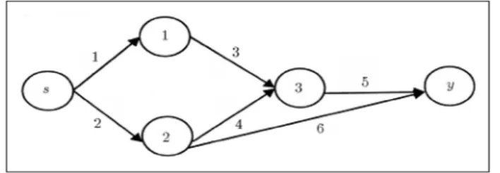
Before proceeding further, the material is illustrated by an example. Consider the network shown in Figure 1. In this example, if activity 3 is dormant, it means that this activity has been nished but the next activity, i.e. 5, cannot begin because activity 4 is still active.
The following denitions help us to identify dor-mant activities more easily.
Denition 3
IfX V, such that s2X andy2X =V X, then, a cut of (s;y) is dened as:
(X;X) =fa2A:(a)2X;(a)2Xg; (4) (X;X) is called a Uniformly Directed Cut (UDC), if (X;X) is empty.
Consider the network of Example 1 shown in Figure 1, again. Clearly, (1,2) is a Uniformly Directed Cut (UDC) because V is divided into two disjoint subsets X and X, where s 2 X and y 2 X. The other UDCs of this network are (2, 3), (1, 4, 6), (3, 4, 6) and (5, 6).
Denition 4
LetD=E[F be a Uniformly Directed Cut (UDC) of a network. Then, it is called an admissible 2-partition, if, for any a 2 F, one has I((a)) 6 F. Actually,
Table1. All admissible 2-partition cuts of the example network.
(1,2) (1,4,6) (3,4,6) (3,4,6) ( ;) (2,3) (1,4,6) (3,4,6) (5,6)
(2,3) (1,4,6) (3,4,6) (5,6) (1,4,6) (3,4,6) (3,4,6) (5,6)
by this denition, in an admissible 2-partition cut, for exampleD=E[F, only the subsetF can be the set of dormant activities.
To illustrate this denition, consider Example 1 again. As mentioned, (3, 4, 6) is a UDC. This cut can be divided into two subsets E and F. For example,
E =f4g and F = f3;6g. In this case, this cut is an admissible 2-partition, because I((3)) = f3;4g6 F and also I((6)) =f5;6g6 F. However, ifE = f6g and F = f3;4g, then, the cut is not an admissible 2-partition, becauseI((3)) =f3;4gF =f3;4g.
Table 1 presents all admissible 2-partition cuts of this network. A superscript star is used to denote a dormant activity. All others are active. As mentioned before, E contains all active while F includes all dormant activities.
LetS denote the set of all admissible 2-partition cuts of the network and S = S [(;). Note that
X(t) = (;) implies that Y(t) = and Z(t) = , i.e. all activities are idle at time t and, hence, the project will be completed by time t. It is proven that fX(t);t0gis a continuous-time Markov process with state spaceS (refer to [6] for details).
As mentioned before,EandF contain active and dormant activities of a UDC, respectively. Suppose activityanishes but there is at least one other unn-ished activity inI((a)), then, this activity moves from
Eto a new dormant activities set, sayF0. On the other hand, let, after processing activity a, its succeeding ones, i.e. O((a)), become active. In this case, all activities of O((a)) will be active and included in a new E0 and the elements of I((a)) will be idle. The elements of the innitesimal generator matrix,
Q= [qf(E;F);(E 0;F0)
g], (E;F) and (E 0;F0)
2S, are calculated as follows:
qf(E;F);(E 0;F0)
g= 8 > > > > > > > > > > > < > > > > > > > > > > > :
a ifa2E;I((a))6F[fag;
E0=E
fag;F 0=F
[fag;
a ifa2E;I((a))F[fag;
E0=E
fag[O((a));
F0=F I((a)); P
a2E
a ifE0 =E;F0=F; 0 otherwise
(5)
In Example 1, if one considers:
E=f1;2g; F = (); E 0 =
f2;3g; andF0 = (), then,E0 = (E
f1g)[O((1)). Thus, from Equation 5,qf(E;F);(E
0;F0) g=
1.
It can be concluded that fX(t);t 0g is a nite-state continuous-time Markov process and, since
qf(;);(;)g = 0, this state is an absorbing state. Obviously, the other states are transient. Furthermore, it is assumed that the states of S are numbered 1;2;;N = jSj, such that this Q matrix becomes an upper triangular one. State 1 is the initial state, namelyX(t) = (O(s);) and stateN is the absorbing state, namelyX(t) = (;).
Let T represent the length of the longest path in the network, or the project completion time in the PERT network. Clearly, T = minft > 0 : X(t) =
N=X(0) = 1g. Thus, T is the time untilfX(t);t0g gets absorbed in the nal state, starting from State 1.
Chapman-Kolmogorov backward equations can be applied to computeF(t) =PfT tg. If one denes:
Pi(t) =PfX(t) =N=X(0) =ig;
i= 1;2;;N; (6)
then,F(t) =P1(t).
The system of linear dierential equations for the vectorP(t) = [P1(t);P2(t);
;PN(t)]T is given by:
P0(t) =QP(t); P(0) = [0;0;:::;1]T: (7)
PROJECT COMPLETION TIME
DISTRIBUTION IN NON-MARKOV
DYNAMIC PERT NETWORKS
The proposed methodology can be easily generalized. Let the new projects be generated, according to a renewal process, with interarrival time distribution
A(t), while the number of servers in each service station is equal to one. Allowing i to be the service rate of
the G=M=1 queueing system settled in the ith node, one can compute 0< x0<1 or the unique root of the following equation by using a numerical method like the Newton-Raphson method:
z= Z
1 0
e it
(1 z)dA(t); 0< z <1: (8) After computing x0, the distribution of time spent in thisG=M=1 queueing system is as follows (see [15] for details).
wi(t) =i(1 x0)e
i (1 x
0
)t; t >0: (9) Thus, the time spent in this service station is exponen-tially distributed with parameteri(1 x0).
The proposed methodology can also be extended to a special class of activity durations with general distributions. In this case, computing the density function of the time spent is quite complicated. Taking this drawback into account and considering that the proposed approach is suitable for Markovian PERT networks, one needs to nd an ecient way to adopt this method for computing the project completion time distribution in general dynamic PERT networks. Therefore, the proposed methodology is extended to activity durations with a generalized Erlang distri-bution with parameters 1;2;
;k(
1 = 2 = =k = in Erlang distributions), but, in heavy trac conditions, which means its utilization factor should approach 1. Moreover, in this case, the new projects should be generated according to a Poisson process.
The expected value () and the variance (2) of the waiting time in a queue in any M=G=1 queueing system, considering the heavy trac condition, are:
t= (E(S) 1)t+o(t);
2t=E(S2)t+o(t); (10)
where S and represent the service time and the arrival rate, respectively (see [15] for more details). The utilization factor is equal to = E(S), which should approach 1. The steady-state density function of the waiting time in queuewq(t) can be approximated
by an exponential with parameter 2
2 (see [15] for more details). Since E(S)<1, then =E(S) 1 is negative and the exponential parameter would be positive, accordingly. Therefore:
wq(t) =
2 2
e(2
2)t; t >0: (11)
One can also decompose the service time with a generalized Erlang distribution into a collection of structured exponentially distributed random variables with parameters j;j = 1;2;;k. Considering GE as a queueing system with a generalized Erlang distribution of service time, nodei, with anM=GE=1 queueing system of orderk, in heavy trac conditions, is replaced with k + 1 exponential serial arcs with parameters ( 2i)=2
i;i1;i2;
;ik. The rst of these k+ 1 exponential serial arcs has a parameter equal to ( 2i)=2
i and the rest have parameters equal
toij;j= 1;2;;k.
Therefore, the proposed algorithm is still ap-plicable in the above general cases. Even if the utilization factor of anM=GE=1 queueing system does not approach 1, the proposed methodology can still be applied, although its accuracy is reduced.
NUMERICAL EXAMPLES
Case I
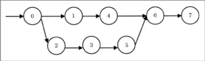
It is of interest to nd the project completion time distribution in a dynamic PERT network, represented as the network of queues depicted in Figure 2. All activity durations, except 6, are exponentially dis-tributed random variables. The duration of activity 6 has an Erlang distribution. Moreover, the new projects, including all their activities, are generated according to a Poisson process with a rate of = 10 per year. Therefore, the arrival stream to each node follows a Poisson process with a rate of 10. The other assumptions are as follows:
1. There is no service station in nodes 0 and 7. It means that there is no predecessor activity for activities 1 and 2 of each new project;
2. There is one server in the service stations, settled in nodes 1, 2 and 3, with the following service rates: (1= 13;2= 15;3= 13);
3. There are an innite number of servers in the service stations, settled in nodes 4 and 5, with the following service rates: (4= 1;5= 2);
4. There is one server in the service station settled in node 6, in which the activity duration has an Erlang distribution with parameters (61;62) = (21;21).
The transformed classical PERT network is de-picted in Figure 3. The parameters of the exponentially distributed arc lengths in this network are computed as explained in previous sections. Since stations 1, 2 and 3 have one server, then, the density function of time spent in each station is (i ). However, since
stations 4 and 5 have an innite number of servers, then, the density function of time spent in each of those stations isi. The waiting time in the queue in
station 6 is approximated exponentially with parameter
Figure2. Dynamic PERT network.
( 26)= 2
6 = 0:741. Moreover, service time in station 6 can be decomposed into two exponential serial arcs. Thus, the parameters of the activities of the network in Figure 3 are as follows:
1= 3; 2= 5; 3= 3; 4= 1;
5= 2; 6= 0:741; 7= 21; 8= 21:
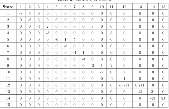
The stochastic process fX(t);t 0g related to the longest path analysis of the transformed classical PERT network of Case I has 15 states. They are in the following order:
S=
(1;2);(1;3);(1;5);(1;5);(2;4);(2;4);(3;4); (3;4);(4;5);(4;5);(4;5);(6);(7);(8)(;) : Table 2 shows the proper innitesimal generator ma-trix,Q, which is constructed from Equations 5.
Finally, Mathematica 5.0 is used to solve the system of dierential Equations 7 and to obtain the project completion time distribution F(t), as below. Figure 4 showsF(t) in Case I.
F(t) =e 21t(0:135e13t 1:12e15t+ 1:064e16t +2:641e17t 5:898e18t+3:665e19t+4:961e20t
6:448e20:25te21t 0:0006t):
Case II
The dynamic PERT network of Case II is also shown in Figure 2. The activity durations of Case II are all
Figure 4. F(t) versustin Case I.
exponentially distributed random variables. Moreover, the new projects are generated according to a renewal process whose interarrival times distribution is Weibull with parameters (;) = (1;2)(A(t) = 1 e t2
). The other assumptions are as follows:
1. There is no service station in nodes 0 and 7; 2. There is one server in all service stations with the
following service rates:
1= 3; 2= 5; 3= 2; 4=4; 5= 7; 6= 2: The transformed classical PERT network of Case II is depicted in Figure 5. The parameters of the exponentially distributed arc lengths in this network are computed as:
1= 2:421; 2= 4:625; 3= 1:216;
4= 3:544; 5= 6:727; 6= 1:216:
Table 2. MatrixQof Case I.
State 1 2 3 4 5 6 7 8 9 10 11 12 13 14 15
1 -8 5 0 0 3 0 0 0 0 0 0 0 0 0 0
2 0 -6 3 0 0 0 3 0 0 0 0 0 0 0 0
3 0 0 -5 2 0 0 0 0 3 0 0 0 0 0 0
4 0 0 0 -3 0 0 0 0 0 0 3 0 0 0 0
5 0 0 0 0 -6 1 5 0 0 0 0 0 0 0 0
6 0 0 0 0 0 -5 0 5 0 0 0 0 0 0 0
7 0 0 0 0 0 0 -4 1 3 0 0 0 0 0 0
8 0 0 0 0 0 0 0 -3 0 3 0 0 0 0 0
9 0 0 0 0 0 0 0 0 -3 1 2 0 0 0 0
10 0 0 0 0 0 0 0 0 0 -2 0 2 0 0 0
11 0 0 0 0 0 0 0 0 0 0 -1 1 0 0 0
12 0 0 0 0 0 0 0 0 0 0 0 -0.741 0.741 0 0
13 0 0 0 0 0 0 0 0 0 0 0 0 -21 21 0
14 0 0 0 0 0 0 0 0 0 0 0 0 0 -21 21
Figure5. Transformed classical PERT network of Case II.
The stochastic process fX(t);t 0g related to the longest path analysis of this transformed classical PERT network has 13 states. They are in the following order:
S=f(1;2);(1;3);(1;5);(1;5
);(2;4);(2;4); (3;4);(3;4);(4;5);(4;5);(4;5);(6)(;)
g: Table 3 shows the corresponding innitesimal generator matrix, Q. Then, F(t) is computed using Mathemat-ica 5.0. Figure 6 showsF(t) in this case.
CONCLUSION
In this paper, an analytical method is developed to compute the distribution function of completion time for any project in a dynamic PERT network with a dedicated resource. The new projects are generated according to a renewal process. The projects share the same facilities and have to wait for processing in a station if the same activity of the previous project is not nished. The proposed methodology can be extended to general activity durations. In this case, it is possible to approximate the service time distribution by an appropriate generalized Erlang distribution. To
Figure6. F(t) versustin Case II.
do that, the rst three moments are matched and then the proposed method is applied to compute the project completion time distribution in the general dynamic PERT network.
The limitation of the proposed method arises from the exponential growth of continuous-time Markov process state space. As the worst case example, for a complete transformed classical PERT network with
l nodes and l(l 1)
2 arcs, the size of the state space is given byN(l) =Ul Ul 1 (refer to [6]) where:
Ul=Xl
k=0
2k(l k): (12)
In practice, the number of arcs is generally much less than l(l 1)
2 and it should also be noted that for large networks, any alternative method of producing reasonably accurate answers will be prohibitively ex-pensive.
Table 3. Matrix Qof Case II.
State 1 2 3 4 5 6 7 8 9 10 11 12 13
1 -7.04 4.62 0 0 2.42 0 0 0 0 0 0 0 0
2 0 -3.64 1.22 0 0 0 2.42 0 0 0 0 0 0
3 0 0 -9.15 6.73 0 0 0 0 2.42 0 0 0 0
4 0 0 0 -2.42 0 0 0 0 0 0 2.42 0 0
5 0 0 0 0 -8.16 3.54 4.62 0 0 0 0 0 0
6 0 0 0 0 0 -4.62 0 4.62 0 0 0 0 0
7 0 0 0 0 0 0 -4.76 3.54 1.22 0 0 0 0
8 0 0 0 0 0 0 0 -1.22 0 1.22 0 0 0
9 0 0 0 0 0 0 0 0 -10.27 3.54 6.73 0 0
10 0 0 0 0 0 0 0 0 0 -6.73 0 6.73 0
11 0 0 0 0 0 0 0 0 0 0 -3.54 3.54 0
12 0 0 0 0 0 0 0 0 0 0 0 -1.22 1.22
Moreover, this paper can be considered as an introduction to the development of proper dispatching rules in dynamic PERT networks, analytically.
REFERENCES
1. Charnes, A., Cooper, W. and Thompson, G. \Critical path analysis via chance constrained and stochastic programming", Operations Research, 12, pp 460-470 (1964).
2. Martin, J. \Distribution of the time through a directed acyclic network", Operations Research, 13, pp 46-66 (1965).
3. Schmit, C. and Grossmann, I. \The exact overall time distribution of a project with uncertain task durations",European Journal of Operational Research, 126, pp 614-636 (2000).
4. Fatemi Ghomi, S.M.T. and Hashemin, S. \A new an-alytical algorithm and generation of Gaussian quadra-ture formula for stochastic network",European Journal of Operational Research,114, pp 610-625 (1999). 5. Fatemi Ghomi, S.M.T. and Rabbani, M. \A new
structural mechanism for reducibility of stochastic PERT networks", European Journal of Operational Research,145, pp 394-402 (2003).
6. Kulkarni, V. and Adlakha, V. \Markov and Markov-regenerative PERT networks", Operations Research, 34, pp 769-781 (1986).
7. Elmaghraby, S. \On the expected duration of PERT
type networks",Management Science,13, pp 299-306 (1967).
8. Fulkerson, D. \Expected critical path lengths in PERT networks",Operations Research,10, pp 808-817 (1962).
9. Robillard, P. \Expected completion time in PERT net-works",Operations Research,24, pp 177-182 (1976). 10. Perry, C. and Creig, I. \Estimating the mean and
variance of subjective distributions in PERT and decision analysis",Management Science,21, pp 1477-1480 (1975).
11. Bock, D.B. and Patterson, J.H. \A comparison of due-date settng resource assignment and job preemption heuristics for the multi-project scheduling problem",
Decision Sciences,21, pp 387-402 (1990).
12. Dumond, E.J. and Dumond, J. \An examination of resourcing policies for the multi-resource problem",
International Journal of Production Management,13, pp 54-76 (1993).
13. Dumond, E.J. and Mabert, V.A. \Evaluating project scheduling and due-date assignment procedures: An experimental analysis",Management Sciences,34, pp 101-118 (1988).
14. Azaron, A. and Modarres, M. \Distribution function of the shortest path in networks of queues", OR Spectrum,27, pp 123-144 (2005).
15. Gross, D. and Harris, M., Fundamentals of Queueing Theory, 2nd Edition, John Wiley & Sons, New York, USA (1985).