Sharif University of Technology
Scientia IranicaTransactions E: Industrial Engineering www.scientiairanica.com
A new bi-objective model for a closed-loop supply chain
problem with inventory and transportation times
F. Forouzanfar
a, R. Tavakkoli-Moghaddam
b;, M. Bashiri
cand A. Baboli
d a. Department of Industrial Engineering, Science and Research Branch, Islamic Azad University, Tehran, Iran. b. School of Industrial Engineering and Center of Excellence for Intelligence Based Experimental Mechanics, College ofEngineering, University of Tehran, Tehran, Iran.
c. Department of Industrial Engineering, Faculty of Engineering, Shahed University, Tehran, Iran. d. DISP Laboratory, INSA-Lyon, 69621 Villeurbanne Cedex, France.
Received 12 October 2014; received in revised form 7 February 2105; accepted 25 April 2015
KEYWORDS Closed-loop supply chain;
Integer nonlinear programming; Transportation; Inventory; Bee algorithm.
Abstract. This paper considers a closed-loop supply chain design problem including several producers, distributors, customers, collecting centers, recycle centers, revival centers, raw materials customers considering several periods, existing inventory and shortage in distribution centers, and transportation cost and time. This problem is formulated as a bi-objective integer nonlinear programming model. The aim of this model is to determine numbers and locations of supply chain elements, their capacity levels, allocation structure, mode of transportation between them, amount of transported products between them, amount of existing inventory, and shortage in distribution centers in each period to minimize the sum of system costs and transportation time in the network. To validate this model and show the applicability of it for small-sized problems, GAMS software is used. Because this given problem is NP-hard, a Bee Colony Optimization (BCO) algorithm is proposed to solve medium and large-sized problems. Furthermore, to examine the eciency of the proposed BCO algorithm, the associated results are compared with the results obtained by the Genetic Algorithm (GA). Finally, the conclusion is provided. © 2016 Sharif University of Technology. All rights reserved.
1. Introduction
Nowadays, rapid economic changes and competitive pressures in current global markets force rms to invest and focus on ecient management of their logistics
system. Return policies, environmental concerns,
and emphasis on servicing and reusing pieces lead to improvement in forwarding traditional supply chain, where Reverse Logistics (RLs) components have been combined. Precise, on time, and accurate transfer of
*. Corresponding author.
E-mail addresses: ie [email protected] (F.
Foroozanfar); [email protected] (R. Tavakkoli-Moghaddam); [email protected] (M. Bashiri);
[email protected] (A. Baboli)
useless materials, items, and products from the end point and ultimate consumer to suitable and relevant unit through supply chain has been described by the term `reverse logistics' [1]. Using reverse logistics not only saves inventory transportation costs, waste material transportation costs, and disposal costs, but also ensures future sale and customer satisfaction. Global competitive conditions, legal obligations, and especially environmental concerns oblige organizations to collect their returned products, so that they revive, recycle, and dispose these products for the sake of environmental conservation. Collecting products after consumption by customers and returning them into supply chain or disposing them have raised the issue of closed loop supply chain, which considers integrated management of forwarding and reverse streams in this
chain. Real design of supply chain network struc-ture leads rms to gain more competitive advantages. Therefore, closed-loop supply chain designing that si-multaneously considers the forward and reverse chains can be ecient in gaining more advantages. Organiza-tions must reduce time and cost of supplying customer demands to survive in global markets. Time for doing the order depends on several factors including a trans-portation state. Dierent transtrans-portation states include a reverse relation between time and cost. Undoubtedly, when this value is slight, it is taken as value added by which one could reach long term and short term competitive advantages in market. On the other hand, decisions regarding the amount of inventory or shortage in Distribution Centers (DC's) in each period, amount of transported products between levels in each phase during each period, and cost of establishing centers with a specic capacity level depend on their costs.
In this paper, we propose a mathematical model for a closed-loop supply chain including several produc-ers, distributors, customproduc-ers, collecting centproduc-ers, recycle centers, revival centers, and raw materials customers. Additionally, we consider several periods, escalating factor of cost, existing inventory and shortage in distribution centers, several levels of capacity and mode of transportation between centers in each period, and transportation cost and time in the modeling as novel innovations. Furthermore, a solution approach based
on the articial bee colony is developed. To the
best of our knowledge, this paper is among the rst publications that consider the bee colony optimization algorithm to solve a closed-loop supply chain network problem. The results of its solution are compared with the results obtained by the Genetic Algorithm (GA). The rest of this paper is organized as follows. In Section 2, the given problem is dened and a mathematical model is proposed. In Section 3, to solve this model, the bee colony optimization algorithm is developed and a genetic algorithm is also applied. In Section 4, some experiments and results are discussed. Finally, conclusion is provided in Section 5.
2. Literature review
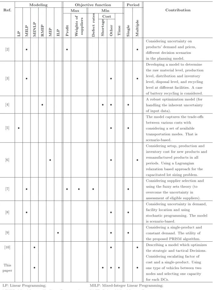
Some studies related to a closed-loop supply chain are mentioned in this section in order to clarify the necessity of this study. Some recent studies on a closed-loop supply chain and characteristics of this paper are illustrated in Table 1.
Tavakkoli-Moghaddam et al. [11] presented a three-level multi-period supply chain model that min-imizes the time and cost of transportation along the chain. They considered existing inventory or shortage in distribution centers and also took into account dierent transportation states between two centers in two dierent levels.
Guide and Van Wassenhove [12] used ve phases to describe the evolution of the closed-loop supply chain research. Krikke et al. [13] surveyed a wide study in the basic closed-loop supply chain about return prac-tices. They analyzed these practices and provided some recommendations for converting value destruction into value creation. Stindt and Sahamie [14] reviewed the research on closed-loop supply chain management in a process industry. They investigated the main characteristic of CLSC planning in the process industry to determine the evolution and gaps of this current research and to explore the topic area and methodology in this eld. Govindan et al. [15] presented a universal literature review of recent papers in a RL/CLSC and suggested future directions and opportunities of related research. According to the reviewed papers, no paper has considered minimization of the cost and transportation time throughout the closed-loop supply chain, simultaneously, so far.
Nature-inspired algorithms are very useful in solv-ing multi-variable optimization problems. The Bee Algorithm (BA) [16] is one of the well-known group algorithms, which simulates the foraging behavior of honey bee colonies. We use the BA for optimizing a closed-loop supply chain network and compare the re-sults with the Genetic Algorithm (GA). The GA [17] is a specic kind of evolution algorithms using biological techniques, such as inheritance and mutation. It is an innovative population based algorithm. This paper is among the rst publications that consider the bee colony algorithm to solve a closed-loop supply chain network problem. Soleimani and Kannan [18] applied a hybrid Particle Swarm Optimization (PSO) and GA for solving a closed-loop supply chain network design problem in large-scale networks. Kannan et al. [19] used a GA to solve a closed-loop supply chain model. Min et al. [20] proposed a mixed-integer nonlinear model and GA to provide a minimum cost solution for the closed-loop supply chain network design problem involving the spatial and temporal consolidations of product returns. To the best of our knowledge, there is no paper that considers the bee colony optimization algorithm to solve a closed-loop supply chain problem. 3. Problem denition
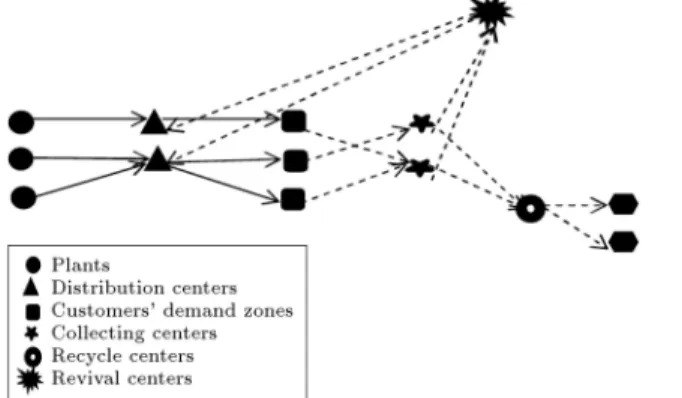
This problem consists of several producers, distrib-utors, customers, collecting centers, recycle centers, revival centers, and raw materials customers (see Fig-ure 1) considering several periods, existing inventory and shortage in distribution centers, and transporta-tion cost and time. Trade-o between cost and time creates a bi-objective problem. One criterion tries to minimize the xed cost for opening centers with a certain capacity level, transportation and allocation costs, construction, process, restructuring and
sepa-Table 1. Some recent studies on a closed-loop supply chain.
Ref.
Modeling Objective function Period
Contribution
LP MILP MINLP RMIP MIP ILP
Max Min
Single Multiple Prot Weigh
ts
of
suppliers Defect
rates
Cost
Time
Shortage Other
[2]
Considering uncertainty on products' demand and prices, dierent decision scenarios in the planning model.
[3]
Developing a model to determine the raw material level, production level, distribution and inventory level, disposal level, and recycling level at dierent facilities. A case of battery recycling is considered.
[4]
A robust optimization model (for handling the inherent uncertainty of input data).
[5]
The model captures the trade-os between various costs with considering a set of available transportation modes. That is scenario-based.
[6]
Considering setup, production and inventory cost for new products and remanufactured products in all periods. Using a Lagrangian relaxation based approach for the capacitated lot sizing problem.
[7]
Considering supplier selection and using the fuzzy sets theory (to overcome the uncertainty in assessment of eligible suppliers).
[8]
Considering uncertainty in demand, facility location and using
stochastic programming. The model is scenario-based.
[9]
Considering a single-product and constant demand. The utility of the proposed PRISM algorithm.
[10] Describing a model which optimizes
the strategic and tactical Decisions.
This
paper
Considering escalating factor of cost and a single-product. Using one type of vehicles between two nodes and selecting one capacity for each DCs.
LP: Linear Programming; MILP: Mixed-Integer Linear Programming; MINLP: Mixed-Integer Nonlinear Programming; RMIP: Relaxed Mixed-Integer Programming; MIP: Mixed-Integer Programming; ILP: Integer Linear Programming.
Figure 1. Closed-loop supply chain network.
ration costs, and inventory and shortage costs in the closed-loop supply chain. The other criterion reduces transportation time along the chain.
3.1. Assumptions
The main assumptions of the presented model are as follows:
1. This problem is single product [21];
2. Several capacity levels are considered for centers and nally one capacity will be chosen for each center;
3. There are several available states for transporta-tion between two consecutive levels [21];
4. Only one kind of transportation vehicles is used between two knots among levels in each pe-riod [21];
5. Faster transportation vehicle is costly [21];
6. There is a balance between inputs and outputs of each center;
7. Several periods are considered along the planning horizon;
8. At the end of the last period, inventory or shortage is supposed to be zero;
9. Centers allocation has been done at the beginning of the rst period and until the end of the planning horizon, it will not change;
10. Shortage in DCs in each period should be given in the next period;
11. The analysis just considers inventory of DCs. 3.2. Sets
I Set of plants;
J Set of DCs;
K Set of demand zones of customers;
L Set of collecting centers;
M Set of revival centers;
N Set of recycle centers;
Di Set of capacity levels available to plant
i (i 2 I);
Dj Set of capacity levels available to
DCj (j 2 J);
Dl Set of capacity levels available to
collecting center l (l 2 L);
Dm Set of capacity levels available to
revival center m (m 2 M);
Dn Set of capacity levels available to
recycle center n (n 2 N);
T Time period.
3.3. Parameters
Bijl1t Time for transporting any quantity
of product from plant i to DCj using
transportation mode l1 in period t;
Bjkl2t Time for transporting any quantity
of product from DCj to customer's
demand zone k using transportation mode l2in period t;
Bkll3t Time for transporting any quantity
of product from customer's demand zone k to collecting center l using transportation mode l3 in period t;
Bln l4t Time for transporting any quantity
of product from collecting center l to recycle center n using transportation mode l4in period t;
Bnel5t Time for transporting any quantity
of product from recycle center n to material customer e using transportation mode l5 in period t;
Blml6t Time for transporting any quantity
of product from collecting center l to revival center m using transportation mode l6in period t;
Bmjl7t Time for transporting any quantity
of product from revival center m to DCj using transportation mode l7 in
period t; Fd
i Yearly xed cost for opening and
operating plant i with capacity level d (d 2 Di); (i 2 I);
Fd
j Yearly xed cost for opening and
operating DCj with capacity level
d (d 2 Dj); (j 2 J);
Fd
m Yearly xed cost for opening and
operating revival center m with capacity level d (d 2 Dm); (m 2 M);
Fd
n Yearly xed cost for opening and
operating recycle center n with capacity level d (d 2 Dn); (n 2 N);
Aijl1t Unit cost of transportation from plant
i to DCj using transportation mode l1
in period t;
Ajkl2t Unit cost of transportation from DCj
to customer's demand zone k using transportation mode l2 in period t;
Akll3t Unit cost of transportation from
customer's demand zone k to collecting center l using transportation mode l3
in period t;
Aln l4t Unit cost of transportation from
collecting center l to recycle center n using transportation mode l4 in
period t;
Anel5t Unit cost of transportation from
recycle center n to material customer e using transportation mode l5 in
period t;
Alml6t Unit cost of transportation from
collecting center l to revival center m using transportation mode l6 in
period t;
Amjl7t Unit cost of transportation from revival
center m to DCj using transportation
mode l7 in period t;
Pi Production cost of each unit of product
in plant i;
Pj Process cost of each unit of product in
DCj;
Pl Process cost of each unit of product in
collecting center l;
Pm Restructuring cost of each unit of
product in revival center m;
Pn Separation cost of each unit of product
in recycle center n;
Vj Holding cost of each unit of inventory
in DCj;
Zj Cost of each unit of shortage in DCj;
ea Cost increase factor for production of
each unit of product in plant i;
eb Cost increase factor for process of each
unit of product in DCj;
ec Cost increase factor for process of each
unit of product in collecting center l;
ef Cost increase factor for restructuring
each unit of product in revival center m;
eg Cost increase factor for separation of
each unit of product in recycle center n;
ev Cost increase factor for holding each
unit of inventory in DCj;
ez Cost increase factor for shortage of
each unit in DCj;
Cet Material customers' demand e in
period t;
lt Un-reviving percentage of collected
products in each collection center l in period t;
wi Capacity of plant i;
wj Capacity of DCj;
wl Capacity of collecting center l;
wm Capacity of revival center m;
wn Capacity of recycle center n;
jt Disrepair percentage of products sent
from DCj in period t;
kt Percentage of supplied demand during
period t which is returned by customer demand of zone k;
Hkt Amount of customer's demand of zone
k in period t;
Lj Initial inventory level in DCj.
3.4. Decision variables
Xijl1t 1 if plant i is allocated to DCj during
period t via transportation mode l1;
and 0, otherwise;
Xjkl2t 1 if DCj is allocated to customer's
demand zone k during period t via transportation mode l2; and 0,
otherwise;
Xkll3t 1 if customer's demand zone k is
allocated to collecting center l during period t via transportation mode l3;
and 0, otherwise;
Xln l4t 1 if collecting center l is allocated
to recycle center n during period t via transportation mode l4; and 0,
otherwise;
Xnel5t 1 if recycle center n is allocated to
material customer e during period t via transportation mode l5; and 0,
otherwise;
Xlml6t 1 if collecting center l is allocated
to revival center m during period t via transportation mode l6; and 0,
otherwise;
Xmjl7t 1 if revival center m is allocated to
DCj during period t via transportation
mode l7; and 0, otherwise;
Ud
i 1 if plant i is opened with capacity
level d; and 0, otherwise; Ud
j 1 if DCj is opened with capacity level
Ud
l 1 if collecting center l is opened with
capacity level d; and 0, otherwise; Ud
m 1 if revival center m is opened with
capacity level d; and 0, otherwise; Ud
n 1 if recycle center n is opened with
capacity level d; and 0, otherwise;
Oijt Amount of product transported from
plant i to DCj during period t;
Ojkt Amount of product transported from
DCj to customer's demand zone k
during period t;
Oklt Amount of product transported from
customer's demand zone k to collecting center l during period t;
Olmt Amount of product transported from
collecting center l to revival center m during period t;
Oln t Amount of product transported from
collecting center l to recycle center n during period t;
Omjt Amount of product transported from
revival center m to DCj during
period t;
Onet Amount of product transported from
recycle center n to material customer e during period t
Qjt Inventory level of DCj in period t;
Ejt Shortage of DCj in period t;
Zkt Amount of supplied demand of
customer in zone k in period t.
3.5. Mathematical model
Minf1 is calculated as shown in Box I, and Minf2 is
obtained by the following equation: minf2=
X
d2Di
X
i
Fd iUid+
X
d2Dj
X
j
Fd jUjd
+ X
d2Dl
X
L
Fd lUld+
X
d2Dm
X
M
Fd mUmd
+ X
d2Dn
X
N
Fd nUnd+
X i X j X l1 X t
Aijl1tXijl1t
+X j X k X l2 X t
Ajkl2tXjkl2t
+X k X l X l3 X t
Akll3tXkll3t
+X L X M X l6 X t
Alml6tXlml6t
+X M X j X l7 X t
Amjl7tXmjl7t
+X L X N X l4 X t
Aln l4tXlml6t
+X N X e X l5 X t
Anel5tXnel5t
+X i X j X t
PiOijt(1 + ea)t
+X j X k X t
PjOjkt(1 + eb)t
+X L X M X t
PlOlmt(1 + ec)t
min f1= max k;t 8 > > > > > > > > > > > > > > > > > > > > < > > > > > > > > > > > > > > > > > > > > : max
j;l2 fXjkl2tTjkl2tg +
" P
j
P
l2
Xjkl2t
# max
i;l1 fXijl1tTijl1tg
+ max
l;l3 fXkll3tTkll3tg +
" P
l
P
l3
Xkll3t
# max l 8 > > > > > > < > > > > > > : " max
N;l4 fXln l4tTln l4tg +
" P
N
P
l4
Xln l4t
# max
e;l5 fXnel5tTnel5tg
# ; "
max
M;l6fXlml6tTlml6tg +
" P
M
P
l6
Xlml6t
# max
j;l7 fXmjl7tTmjl7tg
# 9 > > > > > > = > > > > > > ; 9 > > > > > > > > > > > > > > > > > > > > = > > > > > > > > > > > > > > > > > > > > ; ; Box I
+X L X N X t
PlOln t(1 + ec)t
+X M X j X t
PmOmjt(1 + ef)t
+X N X e X t
PnOnet(1 + eg)t
+X
j
X
t
QjtVj(1+ev)t+
X
j
X
t
EjtZj(1+ez)t;
s.t.: X
L
X
l3
Xkll3t= 1 8k; t; (1)
X
N
X
l4
Xln l4t 1 8l; t; (2)
X
M
X
l6
Xlml6t 1 8l; t; (3)
X
j
X
l2
Xjkl2t= 1 8k; t; (4)
X
N
X
l5
OnetXNel5t Cet 8e; t; (5)
X
L
X
l3
OkltXkll3t ktZkt 8k; t; (6)
X
l3
X
k
ltOkltXkll3t=
X
N
X
l4
Oln tXln l4t 8l; t; (7)
X
l3
X
k
(1 lt)OkltXkll3t=
X
M
X
l6
OlmtXlml6t 8l; t;
(8) X
j
X
l7
OmjtXmjl7t=
X
L
X
l6
OlmtXlml6t 8m; t;
(9) X
l5
X
e
OnetXnel5t
X
L
X
l4
Oln tXln l4t 8n; t;
(10) X
j
X
l1
OijtXijl1t
X
d2Di
Ud
iwi 8i; t; (11)
X
d2Di
Ud
i 1 8i; (12)
X
d2Dj
Ud
j 1 8j; (13)
X
d2Dl
Ud
l 1 8l; (14)
X
d2Dm
Ud
m 1 8m; (15)
X
d2Dn
Ud
n 1 8n; (16)
X
i
X
l1
OijtXijl1t+
X
M
X
l7
OmjtXMjl7t+ Qj(t 1)
X
d2Dj
Ud
jwj 8j; t; (17)
X
d2Dj
Ud jwj
X
k
X
l2
OjktXjkl2t 8j; t; (18)
X
k
X
l3
OkltXkll3t
X
d2Dl
Ud
lwl 8l; t; (19)
X
L
X
l6
OlmtXlml6t
X
d2Dm
Ud
mwm 8m; t; (20)
X
L
X
l4
Oln tXln l4t
X
d2Dn
Ud
nwn; 8n; t; (21)
X
M
X
l7
Xmjl7t=
X
d2Dj
Ud
j 8j; t; (22)
X
M
X
l7
OmjtXmjl7t+
X
i
X
j
OijtXijl1t+ Qj(t 1)
=X
k
X
l2
OjktXjkl2t + Qjt; 8j; t; (23)
X
k
X
l2
(1 jt)OjktXjkl2t Ej(t 1)
+X
l2
X
k
k(t 1)Zk(t 1)Xjkl2t 8j; t; (24)
Qj(t 1)+
X
i
X
l1
OijtXijl1t+
X
M
X
l7
OmjtXMjl7t
X
k
X
l2
HktXjkl2t Ej(t 1)
X
l2
X
k
k(t 1)Zk(t 1)Xjkl2t=Qjt Ejt;
8j; t; (25)
QjT = 0 8j; t; (27)
EjT = 0 8j; t; (28)
QjT0 = L0j 8j; t; (29)
Qjt
X
d2Dj
Ud
jwj 8j; t; (30)
X
l3
X
k
OkltXkll3t=
X
M
X
l6
OlmtXlml6t
+X
N
X
l4
Oln tXln l4t 8l; t (31)
X
l1
Xijl1t 1 8i; j; t; (32)
X
l2
Xjkl2t 1 8j; k; t; (33)
X
l3
Xkll3t 1 8k; l; t; (34)
X
l4
Xln l4t 1 8l; n; t; (35)
X
l5
Xnel5t 1 8n; e; t; (36)
X
l6
Xlml6t 1 8l; m; t; (37)
X
l7
Xmjl7t 1 8m; j; t; (38)
X
j
Xjkl2t= Zkt 8k; t; (39)
Zkt Hkt 8k; t; (40)
Xijl1t;Xjkl2t; Xkll3t; Xln l4t; Xnel5t; Xlml6t; Xmjl7t;
Ud
i; Ujd; Uld; Umd; Und2 [0; 1]; (41)
Oijt; Ojkt; Olmt; Oln t; Omjt; Onet; Qjt; Ejt 0: (42)
In this model, the rst objective function tries to nd the minimum time to transport products along any path in the closed-loop supply chain. The second objective function minimizes the xed cost for opening centers with a certain capacity level, transportation and allocation costs, construction, process, restructur-ing and separation costs, and inventory and shortage costs in a closed-loop supply chain. Constraint (1) shows that each customer's demand zone is allocated to
a collecting center. Constraints (2) and (3) suggest that each collecting center is allocated to a recycle center (in Constraint 2) and a revival center (in Constraint 3) when a collecting center is established. Constraint (4) emphasizes that each customer's demand zone takes service from one DC. Constraint (5) suggests that customer demand for materials is supplied dur-ing each period. Constraint(6) shows the amount of returned product from customer k during period t. Constraints (7) and (8) show that the returned products from customer k to collecting center l are sent to revival center m and recycle center n. Constraint (9) shows that inputs and outputs of the revival center are equal. Constraint (10) indicates that recycled product constituents are sold to customers after recycle process. Constraint (11) relates to the plant capacity. Constraints (12) to (16) show that if a center has been established, a capacity level will be allocated to it. Constraints (17) and (18) relate to capacity of DCj. Constraints (19) to (21) relate to the capacities
of collecting, revival, and recycle centers, respectively. Constraint (22) shows whether DCj is established with
the capacity level and allocated to a revival center. Constraint (23) suggests that the summation of period (t 1) inventory in DCj and products received
from recycle centers and plants during period t is equal to the summation of period t inventory and products sent to the customers' demand zones. Constraint (24) emphasizes that shortage in DCj and impaired sent
products should be compensated in the next phase. Constraints (25) and (26) show that it is impossible to have inventory and shortage, simultaneously, in DCj
in each phase. Constraints (27) and (28) show that in the last period, we do not have inventory and shortage in DCj. Constraint (29) suggests that we consider an
initial inventory level for DCs. Constraint (30) relates to DCj capacity. Constraint (31) indicates that a
revivable part of the collected products from customer k in collecting center l is allocated to a revival center and a recyclable part of it is allocated to a recycle center. Constraints (32) to (38) relate to using one type of transportation vehicles between two centers at two levels. Constraint (39) shows the amount of supplied demand of customer k. Constraint (40) says that this amount cannot be greater than the real demand of customer k. Finally, Constraints (41) and (42) dene variables.
4. Bee colony optimization and genetic algorithms
To show applicability and validity of the presented model, we solve several small-scale problems through a branch-and-bound module in GAMS. This software is a robust tool for solving and analyzing mathematical models of linear and nonlinear optimization problems.
To solve large-scale problems, we use the bee algorithm. In order to show its eciency, the associated results are compared with the results obtained from the genetic algorithm.
4.1. Bee colony optimization algorithm
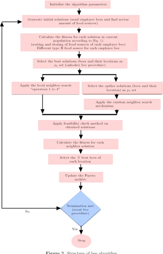
The proposed structure of the bee colony optimization algorithm is as follows (please see Figure 2):
Purposed bee colony optimization algorithm fInitialization:
Initialize the algorithm parameter.
Generate N feasible solutions as the initial population.
While criterion is meet
Calculate the tness for each solution in current population.
Select the best bees and their location as p1 set.
Select the other bees and their location as p2 set.
Apply neighborhood search operator to p1set.
Apply feasibility check method to the obtained solutions.
Assign some bees to the obtained solutions and calculate their tness.
Apply random neighborhood search operator on p2.
Apply feasibility check method on obtained solutions.
Calculate their tness.
Select the N best bees of each location.
Apply improvement method on selected solutions and take
output of this method as population of the next generation.
Update Pareto archive End while
Return the Pareto archive. g
4.1.1. Solution representation
We use a matrix to present each solution. Each
solution includes several matrices which are designed in accordance with model outputs. For example, for variable Xijl1t, we dene a four-dimensional matrix
with dimensions I J l1 T . In the same way, we
dene a matrix for other outputs. 4.1.2. Solution initialization method
Given that the Bee Colony Optimization (BCO) algo-rithm is a population-based algoalgo-rithm, at the beginning of the algorithm, we need a population of solutions as the initial population. This paper uses a random process to produce possible initial solutions. Available solutions indicated by N in each repeat of the BCO process are supposed to be xed during the optimiza-tion process. To produce N possible initial soluoptimiza-tions, the designed process should be repeated N times. 4.1.3. Applicability of solutions
Since during performing the algorithm new solutions are produced, an approach has been designed to check the applicability of solutions. The algorithm make the infeasible solutions to feasible ones where it checks out all the limitations of the produced solutions. If one or more limitations have been violated in that solution, it tries to make the solution feasible.
4.1.4. Fitness function calculation
In this paper, since the proposed model is a multi-objective one, we calculate the tness index of each solution, which classies solutions and calculates the crowding distance criterion of solutions [22]. The tness value of individual c, considering its rank and
objective values, can be calculated by [23]:
Fitnessc= 1
D
P
j=1
2 6 4 fj(c)
Nrank(c)P i=1 fj(i)
3 7
5+(rank(c) 1) D ;
(43)
where D is the number of objectives, fj(i) is the value
of the jth objective of the ith individual, and Nrank(c)
is the number of solutions in rank(c). 4.1.5. Local search (bee P1 group)
To solve the studied problem, a new process is designed based on local search. P1 group solutions population
is the input of this process. This process bases upon neighborhood search. In other words, this process receives group of solutions as input and tries to reach suitable neighbor solutions by recovering each solution. In the present paper, we use a multi-operator local search process as well as a repeatable local search process with guided mutation to design the above process [24]. By combining these two local search processes, we try to present a new process of local search. A general structure of the proposed operator is presented below:
f
Step 1: Get input solutions (p1).
Step 2:
For each solution in p1set, use the multi-operator
search to enhance solutions.
Construct the pool of trial solutions generated in the step before.
g
In this approach, a multi-operator search process is executed on each available solution in P1 group and
the result is a set of local optimized solutions, which are in the neighborhood of the aforesaid solution. All local optimized solutions obtained from execution of this process are pooled. For recovering solutions, their neighborhood is searched and analyzed. Neighborhood search operators used here include an exchange op-erator that will be executed on four location-related matrices. These operators work as follows:
Operator 1: Two indices i and j are constructed randomly during consistent periods f1; ; ng (i.e., n factories) and f1; ; mg (i.e., m distribution centers); index t is produced during period f1; ; T g, and if square Xijl1t is equal to zero, it will be considered
1 and if it is 1, it will be considered zero; also, a stream of materials between factory i and distributor j during period t by vehicle l1 is changed according to
capacities. Then, a modication process is executed on the solution matrices and it modies them according to model limitations.
Operator 2: Two indices k and l are constructed randomly during consistent periods f1; ; kg (i.e., k customer regions) and f1 lg (i.e., l collecting centers); index t is produced during period f1; ; T g and if square Xkll3tis equal to zero, it will be considered
1 and if it is 1, it will be considered zero; also a stream of materials between customer k and collecting center l during period t by vehicle l3 is changed according to
capacities. Then, a modication process is executed on the solution matrices and it modies them according to model limitations.
Operator 3: Two indices l and m are constructed randomly during consistent periods f1; ; lg (i.e., l collecting centers) and f1; ; mg (i.e., m revival cen-ters); index t is produced during period f1; ; T g, and if square Xlml6tis equal to zero, it will be considered 1
and if it is 1, it will be considered zero; also stream of materials between collecting center l and revival center m during period t by vehicle l6is changed according to
capacities. Then, a modication process is executed on the solution matrices and it modies them according to model limitations.
Operator 4: Two indices n and l are constructed randomly during consistent periods f1; ; ng (i.e., n recycle centers) and f1; ; lg (i.e., l collecting cen-ters), index t is produced during period f1; ; T g, and if square Xln l4tis equal to zero, it will be considered 1
and if it is 1, it will be considered zero; also stream of materials between centers l and n during period t by vehicle l4 is changed according to capacities. Then,
a modication process is executed on the solution matrices and it modies them according to model limitations.
Each of these operators search a part of neigh-bor solutions and other parts may be searched by other operators; thus, using one neighborhood search operator may lead to losing some potential neighbor solutions. Therefore, this study uses a multi-operator search process, which will be explained later. In a multi-operator search process, we use the above four operators to produce neighbor solutions. A multi-operator search process algorithm is presented below:
fMulti operator search framework
1. For each input solution x, set papprox= fxg
2. Repeat
3. Randomly select some x in papproxfor which
nh(x) has not been investigated yet 4. For all NR = fnh1; nh2; ; nhrg
Generate neighborhood nhi(x)
5. Update papproxwith all elements xnh in nhi(x)
6. If x in papprox, then
7. Mark x as `investigated'
8. End if
9. Until no element as x in papprox with x still
to be investigated 10. Return papprox
g
In the dened search process, as can be seen in its algorithm, a set of solutions (Papprox) is constructed,
which includes initial solutions. In each repeat of this process, one member that has not been analyzed so far is chosen randomly and neighbor solutions are produced by the aforementioned four neighborhood search operators. Then, approx set P is updated through comparing solutions with non-dominated rela-tions and this cycle will be repeated until all members are analyzed. At the end of the algorithm, approx set P that includes a local optimized solution in the neighborhood of an initial solution is returned as the algorithm result.
4.1.6. Random neighborhood search (P2 group)
To execute random neighborhood search for the second bee group, this study uses a parallel neighborhood search operator. This process uses four operators mentioned in the previous section simultaneously or in a parallel way. If we indicate those operators with ls1,
ls2, ls3, ls4 symbols, the structure of parallel process
is as follows:
fFor input solution s: S1= ls1(s);
S1=Apply feasibility check method on s1;
S2= ls2(s);
S2=Apply feasibility check method on s2;
S3= ls3(s);
S3=Apply feasibility check method on s3;
S4= ls4(s);
S4= Apply feasibility check method on s4;
Output solution = acceptance(s, s1, s2, s3, s4).
g
As can be seen in the above structure, for each existing solution in P2, each operator will be executed
separately on solution and, ultimately, among outputs and inputs of the four operators, one will be chosen, given non-dominated relations, and will be reported as process output.
4.1.7. Selection
In each repeat, the algorithm needs a population of solutions. In this study, for choosing the next repeat population, the existing solutions in the current repeat population and new solutions produced by the algo-rithm are pooled and after classication and calculation of the crowding distance criterion for each solution given its level, through Deb's formula [22], N solutions
which have the highest quality and highest variance will be chosen as the next repeat population of the algorithm.
4.1.8. Improvement structure
In the proposed structure of the bee colony optimiza-tion algorithm, an improvement structure is designed which is executed on the selected solutions in the previous repeat to improve them. Output solutions of the improvement structure are chosen as the next
repeat population of the algorithm. Execution of
the improvement process bases upon Variable Neigh-borhood Search (VNS), as will be explained later. The VNS structure uses four neighborhood search structures. These structures are local search operators, explained in the previous section. These four structures are used in the context of VNS, whose general structure (i.e., pseudo-code) is as follows:
fFor each input solution K = 1
While stopping criterion is met, do New solution=Apply NSS type k
If new solution is better than K = 1 Else,
K = k + 1 If k = 5 then K = 1 End if End if End while g
The VNS algorithm receives all the available solutions in a population and gives an output solution. Then, a recovery process is executed on other solution matrices and after recovery, it replaces the input solution. In fact, a general structure of the recovery process is as follows:
Improvement method
fFor each si in input population
Si=apply VNS procedure on si;
Si=check feasibility method.
g
4.2. Genetic algorithm
The proposed general structure of the genetic algorithm is as follows:
Genetic algorithm fInitialization:
Initialize algorithm parameters;
Generate N feasible solution as the initial population.
While stopping criterion is met, do
Calculate tness for solution in the current population
Calculate number of solutions (nc) for crossover operator.
Counter=0;
While counter nc do Select two parents. Counter=counter+2.
Apply crossover operator on the selected parents. End while
Calculate number of solutions (nm) for mutation operator
Counter=0;
While counter nm do
Select one solution that has not been selected so far. Apply mutation operator on the selected solution. Counter=counter+1;
End while
Apply reproduction operator on the other solutions in
population that has not been selected so far. Select N best solutions as the population of the next generation.
End while
Return the best solution. g
4.2.1. Establishing an initial population Initial solutions are produced randomly. 4.2.2. Parent selection method
This study uses a roulette wheel method for selecting parents. The probability of parallel selection with each chromosome is calculated in terms of its tness. If fk
is the tness value of chromosome k, the probability of parallel survival with that chromosome is as follows:
Pk = Pnfk i=1fi
: (44)
Now, we arrange chromosomes according to Pkand qk,
which are a cumulative frequency of Pk, calculated by:
qk = k
X
i
Pi: (45)
This method simulates a roulette wheel in order to determine which members have a chance to reproduce. Each member in terms of its conformity receives some parts of the rolling wheel. Then, in each phase, one member is selected and this process is subjected to repeat until enough pairs are selected for producing the next generation.
4.2.3. Mutation operator
For executing the mutation operator used in the genetic algorithm, this study uses a parallel neighborhood search structure explained in the bee algorithm.
4.2.4. Crossover operator
The crossover operator designed in this algorithm is a single point crossover operator, which is executed on all solution matrices.
4.2.5. Fitness function
Calculation of the tness value of each solution is similar to the bee algorithm.
4.2.6. Selecting a population for the next repeat At the end of each repeat, among the solutions of that repeat and the new produced solutions, we select n solutions with the highest tness value as a population of the next repeat (or generation).
5. Designing experiment and results
Given the considered hypotheses and parameters of the proposed mathematical model, we dene several small, medium, and large-scale problems, randomly. In order to analyze eciency of the proposed algorithm, we execute it in the MATLAB software environment and results of the execution on experimental problems are compared with the results of GAMS software precise calculations. Comparisons base upon a criterion, which is the gap between target function and execution time of each process.
5.1. Comparison criteria
To solve the presented model, we propose and execute the bee colony algorithm and the genetic algorithm. However, this model is solved in the GAMS software environment. Given that this model is bi-objective, in order to solve the model with GAMS software, we consider the weight composition of targets. To compare the results obtained by the algorithms and GAMS software, we use comparison criterion that shows the gap between target functions. This criterion is explained later.
Eqs. (46) and (47), representing the distance be-tween the proposed optimization algorithms, are used as eciency criterion. This criterion shows validity of the developed algorithms.
error(%) =(ans.BCO ans.GAMS)
ans.GAMS ; (46)
error(%) =(ans.GA ans.GAMS)ans.GAMS : (47)
This criterion is dened as the gap between the objec-tive function values (i.e., weight composition of model objectives) of the algorithm and GAMS software. Eq. (46) calculates the gap between the bee colony algorithm and GAMS software. In this formula, we have:
- ans. BCO: objective function values of the bee colony algorithm;
- ans. GAMS: objective function values of solving the model by GMS software;
- % error: the gap between two objective function
values of the bee colony algorithm and GAMS software.
Eq. (47) calculates the gap between the objective function values of the genetic algorithm and GAMS software. In this formula, we have:
- ans. BCO: objective function values of the genetic algorithm;
- ans. GAMS: objective function values of solving the model by GMS software;
- % error: the gap between two objective function
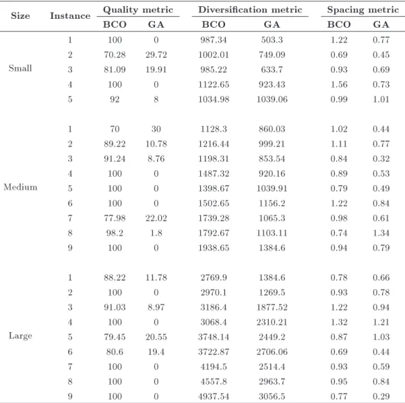
values of the genetic algorithm and GAMS software. In addition to the above criterion and weight composition of objectives, the results of these algo-rithms are compared based on comparison indices of multi-objective problems on the basis of Pareto archive. There are many dierent indices for analyzing quality and variance of multi-objective innovative algorithms. This study considers three comparison criteria pre-sented as follows [25]:
Quality metric: This metric compares the quality of Pareto solutions in each process. Indeed, quality metric classies all the obtained Pareto solutions in both algorithms and indicates what percentage of high level solutions belongs to each process. Higher percentage shows that algorithm has a high quality.
Spacing metric: This metric analyzes the consis-tency of Pareto solution distribution around solutions border. This index is dened by:
s =
PN 1
i=1 jdmean dij
(N 1) dmean :
In this relation, di indicates the Euclidean distance
between two adjacent non-subdued solutions and dmean
shows the average di values.
Diversication metric: This metric is used to de-termine non-subdued solution rate on the optimized border and is dened by:
D =rXN
i=1max(xit yti):
In this relation, kxi
t yitk indicates the Euclidean
distance between two adjacent solutions xi
t and yit on
Table 2. Sizes of some existing problems in the literature. References No. of
plants
No. of DCs
No. of customer's
centers
No. of collecting
centers
No. of revival centers
[26] - - 100 40 30
[27] 20 30 500 -
-[28] - - 120 35
-[29] 3 - - 80 20
[30] 30 40 100 40 30
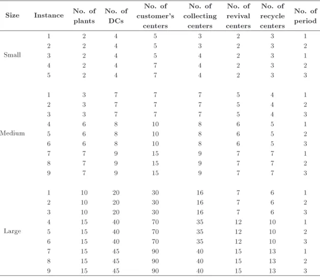
Table 3. Small, medium and large-scale problems. Size Instance No. of
plants
No. of DCs
No. of customer's
centers
No. of collecting
centers
No. of revival centers
No. of recycle centers
No. of period
Small
1 2 4 5 3 2 3 1
2 2 4 5 3 2 3 2
3 2 4 5 4 2 3 1
4 2 4 7 4 2 3 2
5 2 4 7 4 2 3 3
Medium
1 3 7 7 7 5 4 1
2 3 7 7 7 5 4 2
3 3 7 7 7 5 4 3
4 6 8 10 8 6 5 1
5 6 8 10 8 6 5 2
6 6 8 10 8 6 5 3
7 7 9 15 9 7 7 1
8 7 9 15 9 7 7 2
9 7 9 15 9 7 7 3
Large
1 10 20 30 16 7 6 1
2 10 20 30 16 7 6 2
3 10 20 30 16 7 6 3
4 15 40 70 35 12 10 1
5 15 40 70 35 12 10 2
6 15 40 70 35 12 10 3
7 15 45 90 40 15 13 1
8 15 45 90 40 15 13 2
9 15 45 90 40 15 13 3
5.2. Design of experiments
This study presents dierent experimental and real problems with dierent sizes in the area of direct and reverse logistics network design. In order to design and construct experimental problems, we analyze some problems in the literature that are reported in Table 2. Given the existing sizes in the literature, we consider three groups of problems with small, medium, and large sizes to analyze the eciency of the proposed algorithms that are presented in Table 3. For designing experimental problems groups, we try to dene the
problem size according to the existing area in the previous studies as shown in Table 3.
5.3. Parameter setting
The population size in both algorithms is set to 150;
Repeat number (stopping criterion) in both algo-rithms is set to 500;
In GA, crossover rate is considered equal to 0.7 and mutation rate is set to 0.2;
Products transportation time between all centers U[1; 100];
Annual cost of opening centers U[1; 40];
Transportation cost of each unit between all centers U[50; 100];
Costs of production, process, rebuild, separation in their related centers U[1; 20];
Shortage and inventory holding costs in DCs
U[1; 40];
Customers' demand for material e U[1; 20];
Customers' demand U[20; 100];
Initial inventory level U[1; 500];
Capacity of centers in all levels U[1; 1000]. 5.4. Solution results
As can be seen in Table 4, in the rst sample with a small size, error is low and equal to 0.07 per cent for the GA and 0.02 per cent for the BCO algorithm.
Regarding quality, as can be seen, the BCO algorithm can produce higher quality solutions than the GA and GAMS. Regarding time in a proposed structure of the BCO algorithm and using certain search algorithms, time of the BCO algorithm is more than that of the GA and GAMS.
As illustrated in Table 4, one can see that the given problem is more complicated than the existing problems in the literature due to numerous variables. Therefore, GAMS software can solve only small-size problems within an acceptable time, while in large-sized calculation of the exact solution during the rea-sonable time it is not possible. For medium- and large-sized problems, as can be seen in the BCO algorithm, it produces higher quality, but needs much time for solutions as compared to GA. Given the executive results, we conclude that for solving the presented model, the proposed BCO algorithm is more ecient and robust than the GA. As it was mentioned, the results of both algorithms are compared on the basis of Pareto archive using quality, diversication, and space Table 4. Results of small, medium and large-scale problems.
Size Instance OFV CPU time (sec.) Gap (%)
BCO GA GAMS BCO GA GAMS BCO GA
Small
1 1181491 1252640 1152521 395.7 365.17 1 0.02 0.07
2 1226598 1355365 1134969 640.06 578.26 5 0.07 0.16
3 1794968 2028732 1147734 487.5 410.08 42 0.36 0.43
4 1831084 3852185 1041230 1129.8 654.33 780 0.43 0.72 5 3465977 7734957 1701200 1328.05 1012.6 815 0.51 0.78
Medium
1 1387675 1634129 - 1713.8 1467.3 >10800 -
-2 1698359 1895608 - 2011.5 1630.09 >10800 -
-3 1539384 1845281 - 1949.04 1427.3 >10800 -
-4 1787620 1899429 - 2109.01 1511.08 >10800 -
-5 2043612 2403157 - 2017.05 1741.7 >10800 -
-6 1987630 2134252 - 2314.01 1917.06 >10800 -
-7 2529438 2726481 - 2575.1 2113.09 >10800 -
-8 2376948 2859374 - 2719.5 2284.2 >10800 -
-9 2765888 3098100 - 2638.1 2165.01 >10800 -
-Large
1 3487397 3728139 - 3542.1 2871.4 >10800 -
-2 3295429 3295429 - 3792.8 2659.2 >10800 -
-3 3745584 4056711 - 3087.07 2112.3 >10800 -
-4 4082775 5417927 - 4172.7 2978.4 >10800 -
-5 4107439 5672473 - 4587.2 3891.06 >10800 -
-6 4028569 5372876 - 4296.3 3968.5 >10800 -
-7 7907703 9173296 - 5819.09 4275.02 >10800 -
-8 8013319 9826382 - 5569.6 4922.7 >10800 -
-Table 5. Results of small, medium and large-scale problems.
Size Instance Quality metric Diversication metric Spacing metric
BCO GA BCO GA BCO GA
Small
1 100 0 987.34 503.3 1.22 0.77
2 70.28 29.72 1002.01 749.09 0.69 0.45
3 81.09 19.91 985.22 633.7 0.93 0.69
4 100 0 1122.65 923.43 1.56 0.73
5 92 8 1034.98 1039.06 0.99 1.01
Medium
1 70 30 1128.3 860.03 1.02 0.44
2 89.22 10.78 1216.44 999.21 1.11 0.77
3 91.24 8.76 1198.31 853.54 0.84 0.32
4 100 0 1487.32 920.16 0.89 0.53
5 100 0 1398.67 1039.91 0.79 0.49
6 100 0 1502.65 1156.2 1.22 0.84
7 77.98 22.02 1739.28 1065.3 0.98 0.61
8 98.2 1.8 1792.67 1103.11 0.74 1.34
9 100 0 1938.65 1384.6 0.94 0.79
Large
1 88.22 11.78 2769.9 1384.6 0.78 0.66
2 100 0 2970.1 1269.5 0.93 0.78
3 91.03 8.97 3186.4 1877.52 1.22 0.94
4 100 0 3068.4 2310.21 1.32 1.21
5 79.45 20.55 3748.14 2449.2 0.87 1.03
6 80.6 19.4 3722.87 2706.06 0.69 0.44
7 100 0 4194.5 2514.4 0.93 0.59
8 100 0 4557.8 2963.7 0.95 0.84
9 100 0 4937.54 3056.5 0.77 0.29
comparison metrics. The results of these comparisons based on these three metrics are reported in Table 5.
As illustrated in Table 4, in all cases, the proposed BCO algorithm can produce solutions with higher qual-ity and higher diversication than the GA. Regarding the space metric, in most cases, the obtained solutions by the genetic algorithm are more consistent than the obtained solutions of the proposed BCO, which is the disadvantage of BCO.
6. Conclusion
This study has presented a new mathematical model to design a closed-loop supply chain considering sev-eral periods, inventory and shortage in distribution centers, and time and cost of transportation. This problem has been formulated as a bi-objective integer nonlinear programming model, whose applicability has been analyzed by solving several small-sized problems by GAMS software. Because this problem is NP-hard, for solving medium- and large-sized problems, a
Bee Colony Optimization (BCO) algorithm has been proposed and its results have been compared with the results obtained by the Genetic Algorithm (GA). The computational results have indicated that the proposed BCO algorithm produces higher quality so-lutions than the GA; however, its CPU time is not less than that of the GA. Some useful comparison metrics (i.e., quality, space, and diversity metrics) have been applied to validate the eciency of the proposed BCO algorithm. The results have shown that the proposed BCO algorithm produces solutions with higher quality and diversication than the GA; therefore, it is more ecient. The experimental results have indicated that our proposed algorithm outperforms the GA. There are some areas for future research in this paper. A de-terministic model has been developed in this research. It is valuable to consider uncertain parameters in the model and examine the eects of uncertainty on the results. Furthermore, it is worthwhile to apply other multi-objective solution approaches in the literature to solve the model and compare the results.
Acknowledgements
The authors would like to thank the Editor-in-Chief of \Scientia Iranica" and anonymous referees for their helpful comments and suggestions, which greatly im-proved the presentation of this paper. Additionally, the second author would like to acknowledge the partial nancial support of University of Tehran for this research under Grant No. 8106043/1/25.
References
1. Blumberg, D.F. \Introduction to management of re-verse logistics and closed loop supply chain processes", Business & Management, CRC Press, Florida, USA (2005).
2. Amaroa, A.C.S. and Barbosa-Povoa, A.P.F.D. \The eect of uncertainty on the optimal closed-loop supply chain planning under dierent partnerships structure", Computers and Chemical Engineering, 33(12), pp. 2144-2158 (2009).
3. Kannan, G., Sasikumar, P. and Devika, K. \A genetic algorithm approach for solving a closed loop supply chain model: A case of battery recycling", Applied Mathematical Modeling, 34(3), pp. 655-670 (2010).
4. Pishvaee, M.S., Rabbani, M. and Torabi, S.A. \A robust optimization approach to closed-loop supply chain network design under uncertainty", Applied Mathematical Modeling, 35(2), pp. 637-649 (2011).
5. Paksoy, T., Bektas, T. and Ozceylan, E. \Operational and environmental performance measures in a multi-product closed-loop supply chain", Transportation Re-search Part E: Logistics and Transportation Review, 47(4), pp. 532-546 (2011).
6. Zhang, Z.-H., Jiang, H. and Pan, X. \A Lagrangian relaxation based approach for the capacitated lot sizing problem in closed-loop supply chain", Int. J. Production Economics, 140(1), pp. 249-255 (2012).
7. Hassanzadeh Amin, S. and Zhang, G. \An integrated model for closed-loop supply chain conguration and supplier selection: multi-objective approach", Ex-pert Systems with Applications, 39(8), pp. 6782-6791 (2012).
8. Hassanzadeh Amin, S. and Zhang, G. \A multi-objective facility location model for closed-loop supply chain network under uncertain demand and return", Applied Mathematical Modeling, 37(6), pp. 4165-4176 (2013).
9. Subramanian, P., Ramkumar, N., Narendran, T.T. and Ganesh, K. \PRISM: PRIority based simulated annealing for a closed-loop supply chain network de-sign problem", Applied Soft Computing, 13(2), pp. 1121-1135 (2013).
10. Ozceylan, E., Paksoy, T. and Bektas, T. \Modeling and optimizing the integrated problem of closed-loop supply chain network design and disassembly line balancing", Transportation Research Part E: Logistics and Transportation Review, 61, pp. 142-164 (2014).
11. Tavakkoli-Moghaddam, R., Forouzanfar, F. and Ebrahimnejad, S. \A new multi-objective model for a three-level supply chain problem with inventory and transportation times", Proc. of the International Conference on Advances in Supply Chain and Manu-facturing Management (ASCMM), pp. 16-18 (2011).
12. Guide Jr., V.D. R. and Van Wassenhove, L.N. \The evolution of closed-loop supply chain research", Oper-ations Research, 57(1), pp. 10-18 (2009).
13. Krikke, H., Hofenkc, D. and Wang, Y. \Revealing an invisible giant: A comprehensive survey into return practices within original (closed-loop) supply chains", Resources, Conservation and Recycling, 73, pp. 239-250 (2013).
14. Stindt, D. and Sahamie, R. \Review of research on closed loop supply chain management in the process industry", Flexible Services and Manufacturing Jour-nal, 26(1-2), pp. 268-293 (2014).
15. Govindan, K., Soleimani, H. and Kannan, D. \Reverse logistics and closed-loop supply chain: A comprehen-sive review to explore the future", European Journal of Operational Research, 240(3), pp. 603-626 (2015).
16. Pham, D.T., Ghanbarzadeh, A., Koc, E., Otri, S., Rahim, S. and Zaidi, M. \The bees algorithm - A novel tool for complex optimisation problems", 2nd Inter-national Virtual Conference on Intelligent Production Machines and Systems, pp. 454-459 (2006).
17. Goldberg, D.E., Genetic Algorithms in Search, Op-timization, and Machine Learning, Addison-Wesley Longman Publishing Co., Inc., Boston, MA, USA (1989).
18. Soleimani, H. and Kannan, G. \A hybrid particle swarm optimization and genetic algorithm for closed-loop supply chain network design in large-scale net-works", Appl. Math. Modelling, 39(14), pp. 3990-4012 (2015).
19. Kannan, G., Sasikumar, P. and Devika, K. \A genetic algorithm approach for solving a closed loop supply chain model: A case of battery recycling", Applied Mathematical Modelling, 34(3), pp. 655-670 (2010).
20. Min, H., Ko, C.S. and Ko, H-J. \ The spatial and tem-poral consolidation of returned products in a closed-loop supply chain network", Computers & Industrial Engineering, 51(2), pp. 309-320 (2006).
21. Tavakkoli-Moghaddam, R., Forouzanfar, F. and Ebrahimnejad, S. \Incorporating location, routing and inventory decisions in a bi-objective supply chain de-sign problem with risk-pooling", Journal of Industrial Engineering International, 9(19), pp. 1-6 (2013).
22. Deb, K., Pratap, A., Agarwal, S. and Meyarivan, T. \A fast and elitist multi objective genetic algorithm: NSGA-II", IEEE Transactions on Evolutionary Com-putation, 6(2), pp. 182-197 (2002).
23. Enayatifar, R., Youse, M., Abdullah, A.H. and Darus, A.N. \MOICA: A novel multi-objective ap-proach based on imperialist competitive algorithm", Applied Mathematics and Computation, 219(17), pp. 8829-8841 (2013).
24. Qingfu, Zh. And Jianyong, S. \Iterated local search with guided mutation", Proceedings of the IEEE Congress on Evolutionary Computation, pp. 924-929 (2006).
25. Tavakkoli-Moghaddam, R., Azarkish, M. and Sadegh-nejad-Barkousaraie, A. \A new hybrid multi-objective Pareto archive PSO algorithm for a bi-objective job shop scheduling problem", Expert Systems with Appli-cations, 38(9), pp. 10812-10821 (2011).
26. Jayaramann, V. and Srivastava, R. \A closed-loop lo-gistics model for remanufacturing", Journal of the Op-erational Research Society, 50(5), pp. 497-508 (1999).
27. Aras, N., Aksen, D. and Tanugur, A.G. \Locating col-lection centers for incentive-dependent returns under a pick-up policy with capacitated vehicles", European Journal of Operational Research, 191(3), pp. 1223-40 (2008).
28. Gen, M., Altiparmak, F. and Lin, L. \A genetic algorithm for two-stage transportation problem using priority-based encoding", Operations Research, 28(3), pp. 337-354 (2006).
29. Yeh, W.-C. \A hybrid heuristic algorithm for the multistage supply chain network problem", Int. J. Adv. Manuf. Technol., 26(5-6), pp. 675-685 (2005).
30. Jayaraman, V. and Ross, A. \A simulated annealing methodology to distribution network design and man-agement", European Journal of Operational Research, 144(3), pp. 629-645 (2003).
Biographies
Fatemeh Forouzanfar is currently a PhD stu-dent under the supervision of Prof. Reza Tavakkoli-Moghaddam at the College of Industrial Engineering, Iran University of Science and Research in Tehran. She obtained her MSc in Industrial Engineering from the Islamic Azad University of South Tehran Branch in Iran (2011) and her BSc in Industrial Engineering from Iran University of Science and Technology, Behshahr Campus (2007). Her research interests include supply chain and closed-loop supply chain, mathematical mod-eling, and location-routing-inventory problems. Reza Tavakkoli-Moghaddam is a Professor of In-dustrial Engineering at the College of Engineering, University of Tehran in Iran. He obtained his PhD in
Industrial Engineering from Swinburne University of Technology in Melbourne (1998), his MSc in Industrial Engineering from the University of Melbourne in Mel-bourne (1994), and his BSc in Industrial Engineering from Iran University of Science and Technology in Tehran (1989). He serves as a member of Editorial
Board in ve reputable academic journals. He is
the recipient of the 2009 and 2011 Distinguished Re-searcher Awards and the 2010 and 2014 Distinguished Applied Research Awards at University of Tehran, Iran. He has been selected as the National Iranian Distinguished Researcher in 2008 and 2010 by the Ministry of Science, Research, and Technology (MSRT) in Iran. He obtained the outstanding rank as the top 1% scientist and researcher in the world elite group, reported by Thomson Reuters in 2014. He has published 4 books, 15 book chapters, and more than 600 journal and conference papers.
Mahdi Bashiri is an Associate Professor of Industrial Engineering at Shahed University. He holds a BS in Industrial Engineering from Iran University of Science and Technology, MS, and PhD in this eld from Tarbiat Modares University. He is the recipient of the 2013 Young National Top Scientist Award from the Academy of Sciences of the Islamic Republic of Iran. His research interests are facilities planning, meta-heuristics, and multi-response optimization. He published about 19 books and more than 160 papers in reputable academic journals and conferences.
Armand Baboli is an Associate Professor in the De-partment of Industrial Engineering and DISP (Decision and Information for Production System) Laboratory of INSA (National Institute of Applied Sciences) Lyon at the University de Lyon, France. He received his MSc and PhD degrees from Institut National Polytechnique de Grenoble in France, in 1994 and 1999, respectively. His current researches focus on supply chain manage-ment (networks conguration, organization, and coor-dination) under uncertainty, facilities design (layout and location), dynamic cellular manufacturing system, production planning and inventory control, and intel-ligent manufacturing system with mobile robots. He has published more than 110 papers in journals and conferences.