Sharif University of Technology
Scientia IranicaTransactions A: Civil Engineering www.scientiairanica.com
Simulation of ow over a side weir using simulink
A.Y. Mohammed
, A.N. Al-Talib and T.A. Basheer
Department of Dams and Water Resources Engineering, Mosul University, P.O. Box 11244, Mosul, Iraq. Received 10 January 2012; received in revised form 17 July 2012; accepted 4 March 2013
KEYWORDS Side weir; Simulation; Simulink;
Discharge coecient.
Abstract.The present study focuses on the concept of an elementary discharge coecient that is related to the discharge owing through an elementary strip along the side weir length. Simulations of discharge and water depth elevation were done. It is shown that the predicted discharge was in agreement with the one observed, within an error not exceeding 10compared with other works, and was increased when the side weir was installed as oblique against the ow direction.
c
2013 Sharif University of Technology. All rights reserved.
1. Introduction
Weirs are the simplest hydraulic structures used for ow measurement.
A side weir is a weir placed in the wall of a channel over which lateral outow takes place when the water surface in the channel rises above the weir crest. Thus, it is used as a key structure in many hydraulic projects, including irrigation, ood regulation and others.
Chow [1] explains the dierent types of ow pattern passing over a side weir. Subramanya and Awasthy [2], EL-Khashab and Smith [3], Ranga Raju et al. [4], Hager [5] and Singh et al. [6] used experimental results to nd the side weir equation.
Swamee et al. [7] dealt with dierent types of ow diversion structure, and established that the use of an expression for the variation of discharge coe-cient, along with the spatially varied ow equations, is able to represent the diverted ows, satisfacto-rily.
Other investigators, such as Cheong [8], Uyu-maz [9], UyuUyu-maz and Smith [10] and Smith [11], have contributed both experimentally and analytically to
*. Corresponding author.
E-mail addresses: [email protected] (A.Y. Mohammed), [email protected] (A.N. Al-Talib); [email protected] (T.A. Basheer)
the study of ow over side weirs for dierent ow conditions.
The inclined side weir discharge coecient was studied, using a side weir with three dierent crest an-gles, by Mohammed, M.Y. and Mohammed A.Y. [12], and an equation for the discharge coecient was obtained for an inclined side weir.
Paris et al. [13] studied application of the experi-mental observations to the generalized De Marchi [14] hypothesis (1934), which clearly shows that the func-tioning of side weirs on a movable bed can be mod-eled using this hypothesis. These ndings could be instrumental in the design and verication of these structures.
In the present work, a methodology, based on the numerical solution of two ordinary dierential equations for discharge and ow depth simulation using matlab simulink programming, is proposed.
2. Theory and basic equation
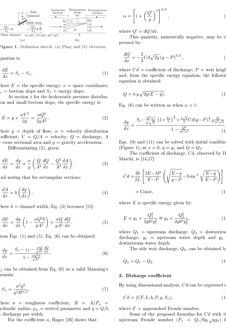
For the equations of spatially varied ow, the energy principle is considered more appropriate, with respect to the momentum approach. However, in the deriva-tion of the energy soluderiva-tion, an estimate of the velocity of lateral outow is necessary. So, it is assumed that this velocity is equal to the cross sectional mean ow velocity [1]. Figure 1 shows a denition sketch in the assumptions of one dimensional ow. The energy
Figure 1. Denition sketch: (a) Plan; and (b) elevation.
equation is: dE
dx = So Sf; (1)
where E = the specic energy; x = space coordinate; So = bottom slope and Sf = energy slope.
At section x for the hydrostatic pressure distribu-tion and small bottom slope, the specic energy is:
E = y +V2g2 = 2gAQ22; (2) where y = depth of ow; = velocity distribution coecient; V = Q=A = velocity; Q = discharge; A = cross sectional area and g = gravity acceleration.
Dierentiating (2), given: dE dx = dy dx+ g Q A2 dQ dx Q2 A3 dA dx : (3)
And noting that for rectangular sections: dA
dx = b
dy dx
; (4)
where b = channel width, Eq. (3) becomes [15]: dE
dx = dy dx
1 QgA23b
+gAQ2dQdx: (5) From Eqs. (1) and (5), Eq. (6) can be obtained:
dy dx =
So sf gAQ2dQdx
1 Q2b
gA3
: (6)
Sf can be obtained from Eq. (6) as a valid Manning's
formula: Sf = n
2q2
y2R4=3; (7)
where n = roughness coecient; R = A=Pw =
hydraulic radius; pw = wetted parameter and q = Q=b
= discharge per width.
For the coecient , Hager [16] shows that:
= " 1 + Q0 q
2#4=3
; (8)
where Q0= dQ=dx.
This quantity, numerically negative, may be ex-pressed by: dQ dx = 2 3Cd p
2g (y P )3=2; (9) where Cd = coecient of discharge; P = weir height, and, from the specic energy equation, the following equation is obtained:
Q = b:yp2g(E y): (10)
Eq. (6) can be written as when = 1: dy
dx =
So Q2n2 b2y103 1+
2y b
4 3+2p2
3 Cd(y P )
3
2 Q
b2y2pg
1 gbQ22y3
: (11) Eqs. (9) and (11) can be solved with initial conditions (Figure 1), at x = 0, y = y1 and Q = Q1.
The coecient of discharge, Cd, observed by De-Marchi, is [14,17]:
Cd =2L3b "
2E 3P E P
s E y
y P 3 sin 1 r
E y E P
!#
+ Const; (12)
where E is specic energy given by: E = y1+ Q
2 1
2gb2y2 1
= y2+ Q 2 2
2gb2y2
2; (13)
where Q1 = upstream discharge; Q2 = downstream
discharge; y1 = upstream water depth and y2 =
downstream water depth.
The side weir discharge, Q3, can be obtained by:
Q3= Q1 Q2: (14)
3. Disharge coecient
By using dimensional analysis, Cd can be expressed as: Cd = f(F; L; b; P; y; So); (15)
where F = approached Froude number.
Some of the proposed formulas for Cd with the upstream Froude number (F1 = Q1=by1pgy1) for
various investigators are shown: Cd = 0:864
1 F2
1
2 + F2 1
0:5
;
(Subramanya & Awasthy [2]); (16) Cd = 0:81 0:6F1; (Ranga Raju et al. [4]);
(17) Cd = 0:45 0:22F2
1; (Cheong [8]); (18)
Cd = 0:485
2 + F2 1
2 + 3F2 1
0:5
; for P = 0;
(Hager [16]); (19)
Cd = 0:33 0:18F1+ 0:49
P y1
;
(Singh et al. [6]); (20)
Cd = 0:71 0:41F1 0:22
P y1
;
(Jalili & Borghei [18]): (21) To solve Eqs. (9) and (11), Cd must be calculated and may be assumed to be a function of head to weir height ratio for a sharp crested rectangular side weir. Swamee [19] has given an equation for a discharge coecient for sharp crested weirs:
Cd =k1
k2
k3+ (y P )=P
k4
+
" (y P )=P (y P )=P + 1
k5# k6
: (22)
4. Experimental verication
Data presented by Al-Talib [20] for water surface elevation were used to study the coecient of discharge in a side weir.
These experiments were performed in the Hy-draulic Laboratory of the Dams and Water Resources Engineering Department at the University of Mosul, Iraq, using a rectangular ume (10 m) long, (0.3 m) wide and (0.45 m) in height. The side channel was (2 m) long, (0.15 m) wide and (0.3 m) in height.
The discharge in the main channel was measured by a sharp crested weir of (0.3 m) distance from the end of the main channel with (10*30*0.1 cm) dimensions. The side weirs were made of wood with (12*15*0.15 cm) dimensions installed at the entrance of the side
channel, inclined at angles of (30, 45, 75 and 90), with
respect to the side channel wall, with ow direction, with ve dierent discharges of (7.3 to 16.5 l/sec). The range of various parameters is given in Table 1. 5. Constancy of energy
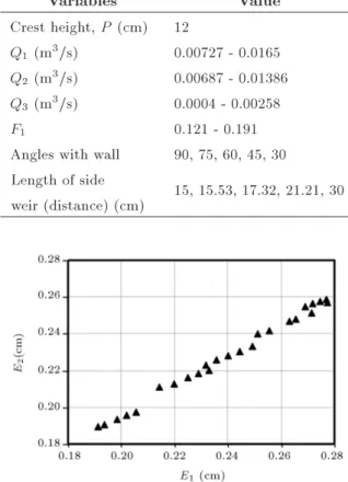
The assumption of constant energy for subcritical ow has to be checked to use the De-Marchi equation. Figure 2 shows that the average energy dierence in the channel between the two ends of the weir (E = E1 E2) is 4.5%. EL-Khashab and Smith [3] estimated
a 5% value for subcritical ow. Thus, the assumption of constant energy is accepted for short sided weirs. 6. Results
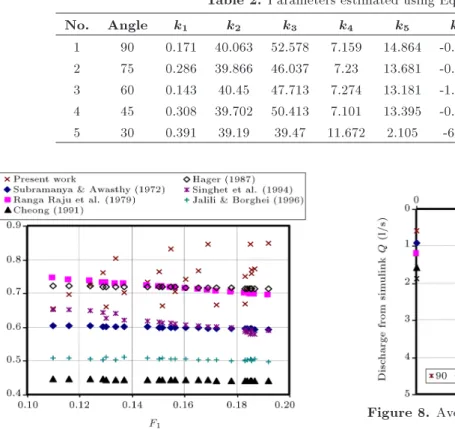
For the data of each run, Eqs. (9) and (11) are solved, and the simulation for discharge and water depth was undertaken using the Simulink package of Matlab Ver. R2010a. Figures 3 and 4 show the discharge and water depth block diagram, respectively. This requires trial values of constants K1 K6, which are estimated using
statistical program SPSS V17 for all cases to be used in Eq. (22). Table 2 shows the constant estimating values; the solution yields y2 and Q2, then, Q3 is obtained
using Eq. (14).
Table 1. Range of parameters measured.
Variables Value
Crest height, P (cm) 12
Q1 (m3/s) 0.00727 - 0.0165
Q2 (m3/s) 0.00687 - 0.01386
Q3 (m3/s) 0.0004 - 0.00258
F1 0.121 - 0.191
Angles with wall 90, 75, 60, 45, 30 Length of side
weir (distance) (cm) 15, 15.53, 17.32, 21.21, 30
Figure 3. Discharge simulink block diagram.
The computed (Q3) weir discharge is then
com-pared with the observed weir discharge (Q3obs) to yield
the average percentage error (E) as: E = 100
N
N
X
i=1
Q3obs. Q3
Q3obs.
: (23)
Figure 5. Observed and calculated discharge.
E was optimized in the weighted least squares sense to minimize it.
Figure 5 shows the observed side weir discharge and the discharge computed by Simulink. It can be seen that the majority of data falls in the error margin of +10%
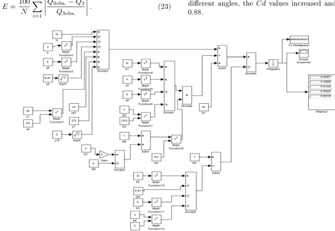
The Cd values computed by Eq. (12) are depicted in Figure 6. It is evident from the scatter that some of the existing approaches are capable of predicting the side weir discharge accurately, especially when the side weir is installed perpendicular to the ow direction. But, when it is installed at an oblique direction with dierent angles, the Cd values increased and reached 0.88.
Table 2. Parameters estimated using Eq. (22).
No. Angle k1 k2 k3 k4 k5 k6 Q3obs (l/s) Error%
1 90 0.171 40.063 52.578 7.159 14.864 -0.685 0.450-1.951 10 2 75 0.286 39.866 46.037 7.23 13.681 -0.839 0..911-2.201 9.85 3 60 0.143 40.45 47.713 7.274 13.181 -1.331 0.955-2.312 9.5 4 45 0.308 39.702 50.413 7.101 13.395 -0.528 1.252-2.555 8.54 5 30 0.391 39.19 39.47 11.672 2.105 -6.55 1.532-2.822 8.443
Figure 6. Compression of discharge coecients equations.
Figure 7. Average depth of ow variation with distance.
Figures 7 and 8 show the average water depth elevation and average ow discharge variation against distance along the longitudinal side weir (x) for all cases (all angles). The average water depth was increased towards the downstream side weir end when the side weir angle increased. While the average discharge decreased towards the downstream side weir end, maximum discharge and water depth occurred when the side weir was installed at an angle (30o)
oblique to the ow direction.
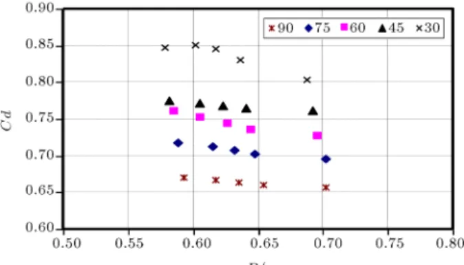
The values of Cd computed by Eq. (22) were plotted against F1, as shown in Figure 9. From this
gure, it is evident that Cd increased when F1and the
oblique angle of the side weir increased.
To study the eect of parameter P=y1 on the
Figure 8. Average ow variation with distance.
Figure 9. Discharge coecient variation with Froude number.
discharge coecient, Cd values were plotted against P=y1in Figure 10. The gure reveals that Cd decreases
with increased P=y1, and increased when the side weir
installed angle increased.
The results, as shown in Figures 11 and 12, represent the simulation of discharge and water depth. It appears that increasing discharge and water depth with time and side weir installed angles increases. 7. Conclusions
In this study, the elementary side weir discharge has been described with the coecient of discharge model for an oblique side weir. Comparison of predicted and observed discharge shows the validation of the model
Figure 10. Discharge coecient variation with P=y1.
Figure 11. Side discharge simulink test results.
Figure 12. Water depth simulink test results.
in the simulation of discharge and water surface prole equations with Matlab Simulink.
The maximum discharge and water depth oc-curred when the side weir was installed at an angle (30) oblique to the ow direction, with a majority
er-ror width of +10% for the observed side weir discharge and the discharge computed by Simulink.
The Cd values computed by Eq. (12) increased to 0.88 when the weir was installed at an oblique direction with dierent angles.
References
1. Chow, V.T., Open Channel Hydraulics, McGraw-Hill, New York (1959).
2. Subramanya, V. and Awasthy, S.C. \Spatially varied owover side weirs", Journal of Hydraulic Division, ASCE, 98(1), pp. 1-10 (1972).
3. EL-Khashab, A. and Smith, K. \Experimental inves-tigation of ow over side weirs", Journal of Hydraulic Division, ASCE, 102(9), pp. 1255-1268 (1976). 4. Ranga Raju, K., Prasad, B. and Gupta, S.K. \Side
weir in rectangular channel", Journal of Hydraulic Division, ASCE, 105(5), pp. 547-554 (1979).
5. Hager, W.H. \Lateral outfow over side weirs", Journal of Hydraulic Engineering, ASCE, 113(4), pp. 491-504 (1987).
6. Singh, R., Manivannan, D. and Satynarayana, T. \Dis-charge coecient of rectangular side weirs", Journal of Irrigation and Drainage Engineering, ASCE, 120(4), pp. 814-819 (1994).
7. Swamee, P.K., Pathak, S., Mohan, M., Agrawa, L.S. and Ali, M. \Subcritical ow over rectangular side weir", Journal of Hydraulic Engineering, ASCE, 120(1), pp. 212-217 (1994).
8. Cheong, H. \Discharge coecient of lateral diversion from trapezoidal channel", Journal of Irrigation and Drainage Engineering, ASCE, 117(4), pp. 461-475 (1991).
9. Uyumaz, A. \Side weir in U-shaped channels", Journal of Hydraulic Engineering, ASCE, 123(7), pp. 639-646 (1997).
10. Uyumaz, A. and Smith, K. \Design procedure for ow over side weirs", Journal of Irrigation and Drainage Engineering, ASCE, 117(1), pp. 79-90 (1991). 11. Smith, K. \Coputer programing for ow over side
weirs", Journal of Hydraulic Engineering, 99(4,3) Pro-ceedings paper 9626 (1973).
12. Mohammed, M.Y. and Mohammed, A.Y. \Discharge coecient for an inclined side weir crest using a constant energy approach", Flow Measurement and Instrumentation, 22(6), pp. 495-499 (2011).
13. Paris, E., Solari, L. and Bechi, G. \On the applicability of the De Marchi hypothesis for side weir ow in the case of movable beds", Journal of Hydraulic Engineer-ing, ASCE, 138(7), pp. 653-656 (2012).
14. De Marchi, G. \Saggio di teoria del funzionamento degli stramazzi laterali", Energ. Elettr., 11(11), pp. 849-860 (1934).
15. Venutelli, M. \Method of solution of nonuniform ow with the presence of rectangular side weir", Journal of Irrigation and Drainage Engineering, ASCE, 134(6), pp. 840-846 (2008).
16. Hager, W.H. \The hydraulics of distribution chan-nels", Part 1-2, Communications from the Laboratory of Hydraulics, Hydrology and Glaciology, No. 55-56, Zurich, Switzerland (1982).
17. Henderson, F., Open Channel Flow, Macmillan, New York, N.Y. (1966).
18. Jalili, M. and Borghei, S. \Discussion of discharge coecient of rectangular side weir by Singh D. Main-vannan and Satyanareyana", Journal of Irrigation and Drainage Engineering, ASCE, 122(2), p. 132 (1996). 19. Swamee, P.K. \Generalized rectangular weir
equa-tions", Journal of Hydraulic Engineering, ASCE, 114(8), pp. 945-949 (1988).
20. Azza N. Al-Talib \Flow over oblique side weir", Dam-ascus University Journal, 28(1), pp. 15-23 (2012).
Biographies
Ahmed Younis Mohammed received a BS degree in Irrigation and Drainage Engineering, in 1996, and a MS degree in Hydraulics Engineering, in 2002, respectively, from the Department of Engineering at the University of Mosul, Iraq. He is currently Assistant Professor in the Dams and Water Resources Department. His research interests include Hydraulics, open channel hydraulics, dams, weirs, sluice gate, water resources, hydraulics and water resources programming. He is also author of many publications.
Azza Nasir Allah AlTalib received a BS degree in Irrigation and Drainage Engineering, in 2000, and a MS degree in Hydraulics Engineering, in 2007, respectively, from the Department of Engineering at the University of Mosul, Iraq. She is currently a Lecturer in the Dams and Water Resources Department. Her research interests include Hydraulics, open channel hydraulics, dams, weirs, sluice gates, and water resources. She is also author of many publications.
Tallal Basheer Ahmed received a BS degree in Irrigation and Drainage Engineering, in 1990, and a MS degree in Hydraulics Engineering, in 1996, respectively, from the Department of Engineering at the University of Mosul, Iraq. He is currently a PhD degree student in UPM University, Putra Malaysia, and has worked as a Lecturer in the Dams and Water Resources Department since 2004. His research interests include Hydraulics, open channel hydraulics, dams, weirs, sluice gate, and water resources. He is also author of many publications.