Chemical potential beyond the quasiparticle mean field
N. Dinh Dang1,2,*and N. Quang Hung1,†
1Heavy-Ion Nuclear Physics Laboratory, RIKEN Nishina Center for Accelerator-Based Science, 2-1 Hirosawa,
Wako City, 351-0198 Saitama, Japan
2Institute for Nuclear Science and Technique, Hanoi, Vietnam
(Received 15 September 2009; revised manuscript received 11 November 2009; published 4 March 2010)
The effects of quantal and thermal fluctuations beyond the BCS quasiparticle mean field on the chemical
potential are studied within a model, which consists ofNparticles distributed amongstdoubly folded equidistant
levels interacting via a pairing force with parameterG. The results obtained at zero and finite temperatures
T within several approaches, which include the fluctuations beyond the BCS theory, are compared with the
exact results. The chemical potential, defined as the Lagrangian multiplier to preserve the average number of particles, is compared with the corresponding quantity, which includes the effect from fluctuations of particle and quasiparticle numbers beyond the BCS quasiparticle mean field. The analysis of the results shows that the latter
differs significantly from the former as functions ofGandT. The chemical potential loses its physical meaning
in the system with a fixed number of particles or after eliminating quantal fluctuations of particle (quasiparticle) numbers by means of particle number projection. The validity of the criterion for the signature of the transition to Bose-Einstein condensation, which occurs in infinite systems when the chemical potential hits the bottom of the energy spectrum, is reexamined for the finite multilevel model.
DOI:10.1103/PhysRevC.81.034301 PACS number(s): 21.60.Jz, 24.10.Pa, 24.60.Ky
I. INTRODUCTION
Fluctuations play an important role in small finite systems such as atomic nuclei. The mean-field theories, which work well for very large or infinite systems in condensed matter and solid state physics, need to be modified when applied to atomic nuclei, especially the light ones. Among these theories, the most popular one is the BCS theory, which describes the phe-nomenon of superconductivity (superfluidity). It is well known that this theory violates the particle number, which causes the quantal particle-number fluctuations (PNFs). At finite temperature (T =0), the BCS theory also violates the unitarity relation R2=R for the generalized single-particle density
matrixR. It has been shown by Goodman [1] that this sym-metry violation comes from the effects due to quasiparticle-number fluctuations (QNF), which are neglected within the Hartree-Fock-Bogoliubov (HFB) theory at T =0. The PNF are of the quantal nature as they exist even atT =0, whereas the QNF are thermal fluctuations because they arise only at
T =0.
The results of a considerable number of theoretical studies have shown that fluctuations in small systems indeed lead to significant modifications of quantities, which are defined within the mean field and/or thermal equilibrium, where the effects of fluctuations are ignored. Among the two unknowns, which are defined by solving the BCS equations, namely the pairing gap and chemical potential, much attention has been devoted so far to the study of the first one, the pairing gap. It has been shown, for instance, that removing quantal fluctuations by using various methods of particle-number projection (PNP) significantly improves the agreement between the theoretical
†On leave of absence from the Institute of Physics, Hanoi, Vietnam;
predictions and experimental data on pairing energies. The PNP also eliminates the shortcoming of the BCS theory, which breaks down at small valuesGGcof the pairing interaction
parameter, where the BCS equations have only trivial solutions [2–4]. AtT =0, the results of theoretical studies in the last three decades have also shown that thermal fluctuations smooth out the sharp transition between the superfluid phase to the normal one (the SN phase transition) in nuclei [5–10]. In very large or infinite systems, the SN phase transition takes place when the superfluid pairing gap(T) collapses at a critical temperature Tc0.57(0), where (0) is the value of the
pairing gap atT =0. However, in small systems such as nuclei, under the effects of thermal fluctuations, namely the QNF, the pairing gap never collapses, but decreases monotonously with increasingT.
The second quantity, the chemical potential, describes the change in energy when one particle is added to the system at constant entropy and volume. In nuclear physics, the vanishing of chemical potential indicates the vicinity of the nucleon drip line. In the study of Bose-Einstein condensation (BEC), as has been shown by Nozi`eres and Schmitt-Rink (NSR) [11], one expects the system to undergo the BEC into a single quantum state with zero total momentum when the chemical potential of the bound pair of fermions reaches the bottom of the bound state band. The aim of the present article is to study the effects of quantal and thermal fluctuations on the chemical potential and some of their consequences within the exactly solvable multilevel pairing model, which is also called the ladder, picket-fence, or Richardson model.
II. CHEMICAL POTENTIAL
The chemical potential has been first defined by Gibbs as the energy, which is required to add an infinitesimal quantity of a substance to any homogeneous mass, divided by the quantity of the substance added. This energy increase should not change the volume and entropy of the homogenous mass. Applied to the many-body systems, the chemical potential µ is the minimum energy required to add a particle to a system in thermal equilibrium with the heat bath. This condition requires that the grand potential (µ, T)≡F −µN of the system, whose average number of particles is equal toN, reaches the minimum, that is,
δ(µ, T)=δF −µδN =δE−T δS−µδN =0, (1)
whereF =E−T Sis the Helmholtz free energy,Eis the total (internal) energy,S is the entropy, and T is the temperature of the system. From Eq. (1) it follows that the thermodynamic chemical potentialµof a system with the average numberN
of particles at a constant volume and temperature is given as
µ= ∂F
∂N. (2)
In the case when the free energyF is a quadratic function of
N, the definition Eq. (2) gives the same result as that obtained by using the arithmetic average,
µ= 12[µ(+)+µ(−)], (3)
whereµ(+)andµ(−)are the chemical potentials defined as half
of the energy required to add two particles to a system withN
andN−2 particles, respectively,
µ(+) =12[F(N+2, )−F(N, )], µ(−) =1
2[F(N, )−F(N−2, )], (4)
wheredenotes the number of single-particle levels (the size of the system). This leads to
µ=1
4[F(N+2, )−F(N−2, )]. (5)
At T = 0, the entropy S vanishes, so that the free energy
F(N, ) reduces to the ground-state energy Eg.s(N, ), and
Eq. (5) turns to the conventional approximation for the chemical potential at zero temperature.
It is worth emphasizing that the concept of chemical potential µ is meaningful only in the presence of PNF. Therefore, at finite temperature,µis defined within the grand canonical ensemble (GCE), where not only the energy, but also the particle number is allowed to fluctuate so that the variation over δN is possible. To get more insight into this issue we recall that an alternative quantity, which represents the effort of adding an extra particle to the system, is called the fugacity
f, whose logarithm is equal to the thermodynamic chemical potentialµ, that is,
µ=Tlnf, or f =eβµ, β =T−1. (6)
An average quantity, such as the energyE, particle numberN, and, consequently, the chemical potentialµitself, is calculated within the GCE as a weighted sum over systems with different numbers of particles. The weight is given by the grand partition
functionZ(β, µ). The latter is defined as
Z(β, µ)= ∞
n=0
fnZn(β), Zn(β)=e−βE
(n)
, (7)
whereZn(β) is the partition function of the canonical ensemble
(CE) of the system withnparticles. Indifferent of the GCE, within the CE only the energy is allowed to fluctuate whereas its particle number is fixed. The GCE becomes the CE if there is no PNF, that is, no summation takes place over the particle numbers at the right-hand side of Eq. (7). In this case, Eq. (7) reduces to Zn=N(β, µ)=fNZN(β). Because at a fixed N,
one should have ZN(β, µ)=ZN(β), it follows that fN =
1, or µ= 0 within the CE. This argument shows that the chemical potential is a meaningful concept only within the GCE. Therefore, although the free energyF can be calculated exactly within the CE, where no PNF are allowed, the result for the chemical potentialµobtained from the definition Eq. (2) or the approximation Eq. (5) already involves several CEs with different numbers of particles, for example,n=N, andN ±2 in Eq. (5) (i.e., assuming the existence of PNF).
A. Within quasiparticle mean field
The present article considers the pairing Hamiltonian,
H =
j m
ja†j maj m−G
jj
mm>0
aj m† aj†majmajm. (8)
It describes a system of N particles with single-particle energies j, generated by the particle creation operators a†j m on jth orbitals with degeneracies 2j (j =j+
1/2), and interacting via a monopole-pairing force with the parameterG. The symboldenotes the time-reversal operator, namelyajm=(−)j−maj−m. The eigenvalues and eigenvectors
of this pairing Hamiltonian can be found by exact diagonal-ization [12]. Thed(n)
s -degenerated eigenvaluesEs(n), obtained
for the system withnparticles, are used to construct the grand partition functionZ(β, µ), which is employed to calculate the exact GCE total (internal) energy as [13]
Eexact=
1
Z(β, µ)
s,n
E(n)
s f
nZ
n(β), Zn(β)=
s
ds(n)e−βEs(n).
(9) The GCE sum in Eq. (9) is carried out over alln=1,. . .,-1 with blocking properly taken into account for oddn. From the exact GCE total energy Eexact, one calculates the entropy by
using the Clausius definition,δS =βδE, which leads to
S=
T
0
1
τ ∂E
∂τdτ. (10)
Consequently the free energy F is known, from which the exactµcan be estimated according to the definition Eq. (2) or approximation Eq. (5).1
1Notice that, when the grand partition function is known, one can use
the differentials of lnZ(β)αto obtain the entropyS=β(E−µN)+
lnZ(β, µ), which is equivalent to Eq. (10) (see Eqs.
For a system with a given numberN of particles such as an atomic nucleus, the chemical potential is often defined as a Lagrangian multiplierλenforcing the constraint of density normalization, namely,
δ
F[fi]−λ
i
fi−N
=0, (11)
where fi are the occupation numbers. This leads to the
variational procedure,
(δF[fi]/δfi)|fi=fi0 =λ, (12)
wherefi0are the reference occupation numbers that minimize the energy. Definition Eq. (12) to determine the chemical po-tentialλis often used within the BCS-based approaches, where the single-particle mean field and the pairing correlations are unified into the quasiparticle mean field. The total energyEand the particle-number constraint are calculated as the expectation values of the pairing HamiltonianH (8) and particle-number operator ˆN, respectively, namely
E= H, N = Nˆ, (13) where the symbol. . .denotes the average within the GCE at a given temperatureT =0. AtT =0 this GCE average is replaced with the expectation value in the ground state. The variational procedure is carried out within the quasiparticle representation H of the Hamiltonian H, which is obtained by expressing the particle operators,aj†andaj, in the pairing
HamiltonianH[Eq. (8)] in terms of the quasiparticle ones,αj†
andαj by using the canonical Bogoliubov transformation: aj m† =ujα†j m+vjαjm, ajm=ujαjm−vjαj m† . (14)
The explicit form ofHcan be found in many references, for example, Eqs. (3)–(14) of Ref. [15]. The variational variables are the coefficients uj and vj, whereas the variation of the
entropy over the quasiparticle occupation number nj yields
the explicit expression for nj in the form of Fermi-Dirac
distribution of noninteracting quasiparticles,
nj =
1
eβEj +1, (15)
withEj being the quasiparticle energies. As the result of this
variational procedure, the BCS equations are obtained, which determine the pairing gap and the Lagrangian-multiplier chemical potentialλfor a given single-particle spectrum with energiesj at a given valueG, namely,
=
j
jujvj(1−2nj), (16)
N =2
j
j
(1−2nj)vj2+nj . (17)
calculations using the exact eigenvalues of the pairing Hamiltonian as it is free from errors caused by calculating numerically the derivative under the integration in Eq. (10).
The Bogoliubov’s coefficientsuj andvj have now the explicit
form,
u2j = 1
2
1+
j−λ Ej
, vj2= 1
2
1−
j −λ Ej
, (18)
with the quasiparticle energiesEj and single-particle energies j, renormalized by the self-energy term−Gv2
j,
Ej =
(j −λ)2+2,
j =j −Gvj2. (19)
B. Beyond quasiparticle mean field
Within the quasiparticle mean field, the two ways of calculating the chemical potential, either by using definition Eq. (2) for µ or as the Lagrangian multiplier λ from the variational Eq. (12), produce the same result (i.e., µ=λ). However, it is well known that the BCS theory violates the particle number. The chemical potential λ found as the Lagrangian multiplier within the BCS theory ensures only the particle-number conservation in average [see Eq. (13)], just ignoring the effects caused by PNF,
δN2≡ Nˆ2 −N2=0. (20)
AtT =0, besides the quantal fluctuations of particle number, there appears the QNF as well,
δN2≡
j
δNj2=
j
nj(1−nj)=0, (21)
which are also neglected in the BCS theory at T =0. The present section discusses the effects of these fluctuations on the chemical potential.
1. Effects of particle-number fluctuations within Lipkin-Nogami method
To eliminate the PNF, one has to carry out the PNP. The Lipkin-Nogami (LN) method [2] is a perspicacious approximate PNP before variation, which has been widely applied in calculations for realistic systems [16]. It proposes a variational procedure based on a trial HamiltonianHLNin the
form,
HLN=H−λ1Nˆ −λ2Nˆ2, (22)
instead ofH−λNˆ. As the result, the LN equations, obtained for the pairing gap and particle number, are formally the same as the BCS ones, Eqs. (16) and (17). However, the chemical potentialλis now replaced with its corresponding LN value,
λLN,
λLN=λ1+2λ2(N+1), (23)
whereas the LN renormalized single-particle energies, (j)LN=j +4λ2vj2=j+(4λ2−G)v2j, (24)
according to the minimization Eq. (1) and definition Eq. (2), is equal to
µLN=
δFLN
δN =
δ(ELN−T S)
δN =λ1+2λ2N =λLN−2λ2.
(25) The quantity λLN can be defined as the modified chemical
potential beyond the BCS quasiparticle mean field to em-phasize the fact that it takes into account the effects due to
δN2, which is neglected within the BCS theory, although this
definition should be taken with a grain of salt. Indeed, as the LN method is an approximate PNP, it partially restores the exact particle number (i.e., eliminating the PNF). An exact PNP would eventually conserve the particle number exactly, (i.e., it would eliminate completely the PNF). At T =0, for example, the exact PNP would bring the GCE results back to the CE ones. In the latter case, the thermodynamic chemical potential µ becomes completely irrelevant as has been discussed previously. Therefore, strictly speaking, in the presence of PNF, only the quantityµLN, which neglects
the effects due toδN2, preserves the full meaning of a true
thermodynamical potential, notλLN.2 The total energyELNis given as
ELN=E−λ2δN2. (26)
The explicit expression of the PNFδN2is given by Eqs. (15)–
(17) in Ref. [17], whereasEhas the same form as that obtained within the BCS theory. The parameterλ2is not a Lagrangian multiplier, but defined so thatHLNNˆ2N =0. This leads to
λ(2i)= 1
2
∂2E(i−1)
∂N2 , (27)
where the superscript i denotes the ith iteration, at which
λ2converges to the desired accuracy. The explicit expression
of λ2 at finite T is given in Ref. [15]. At T = 0, the
quasiparticle occupation numbersnj vanish, so one recovers
from Eqs. (16), (17), and (27) the zero-temperature LN equations, and the expression forλ2atT =0 [2], respectively.
The trial HamiltonianHLN(22) is, in fact, the first order of
the infinite expansion series,
H∞=H−
∞
j=1
λjNj, (28)
which contains all higher-order PNF such asδNj = Nˆj −
Nj withj >2 as well. By neglecting the effect ofδNj and
taking the variation according to Eq. (1), this infinite series
2In a similar manner, the pairing gap is a mean-field concept with
its true meaning only within the BCS theory. This gap collapses at aT =Tc forG > Gc or at anyG < Gc. Meanwhile, the exact solutions of the pairing problem produce no pairing gap, but only pairing correlation energy, from which one can define the “exact”
pairing gap. The latter, however, never collapses at anyT andG. The
approaches, which take into account thermal fluctuations beyond the quasiparticle mean field [5,6,8–10,18], also lead to the pairing gap
that does not collapse atT > Tc, as has been discussed in Sec.I.
would eventually yield the new thermodynamic chemical potentialµ∞in the form,
µ∞=λ1+
∞
j2
jλjNj−1. (29)
Similar toµLN, this thermodynamic chemical potentialµ∞is different fromλ∞=µ∞+2λ2+ · · · , which is the quantity that includes all quantal effects due to PNF beyond the BCS quasiparticle mean field.
2. Effects of quasiparticle-number fluctuations within
LN1+SCQRPA and MBCS theories
The effects of QNF are taken into account in a microscopic way within two recent approaches, called the modified BCS (MBCS) theory [9,10] and the Lipkin-Nogami plus self-consistent quasiparticle random-phase approximation (LN1+SCQRPA) [15]. Although both the LN1+SCQRPA and MBCS theories take the effects of QNF into account microscopically, they are based on different assumptions. The details of these approaches have been discussed thoroughly in Refs. [9,10,15,18], therefore, only the main results, nec-essary for the analysis in the present article, are summarized below.
(a) LN1+SCQRPA. The LN1+SCQRPA uses the same variational procedure as that employed for the derivation of the BCS and/or LN equations. However, it retains the expectation values ofA†jA†j,A†jAj, andNjNj, withA†j ≡[α
†
j ⊗
α†j]00/√2 andNj =
mα†j mαj m. These expectation values are
neglected within the BCS and LN theories. As the result, within the LN1+SCQRPA one obtains a generalized level-dependent gap equation,
j =
G
Dj
j
jDjDjujvj, Dj =1−N j
j
. (30)
The expectation value of the product of two quasi-particle density operators at the right-hand side of Eq. (30) is calculated approximately by using the exact relation,
DjDj = DjDj + δNjj
jj
,
with δNjj = NjNj − NjNj, (31)
and the mean-field contraction,
δNjj 2jδNj2δjj, δNj2≡nj(1−nj), (32)
with the quasiparticle occupation numbernj,
nj =N
j
2j
=1
2(1− Dj). (33) As the result, the gap equation [Eq. (30)] is split to a sum of a quantal level-independent part, , and a thermal level-dependent part,δj, namely,
where
=G
j
jujvj(1−2nj), δj =2G δNj2
1−2nj ujvj.
(35) The expression of the gap j differs from that of the BCS
(LN) gap by the level-dependent partδj, which contains the
QNFδNj2on thejth orbital. The corrections due to coupling to the SCQRPA pair vibrations enter in the expression of the renormalized single-particle energies, which are now given as
(j)LN1+SCQRPA=j +
G
j(1−2nj)
j
j
u2j−v2j
×(A†jA†j=j + A †
jAj), (36)
where the expectation values A†jA†j and A†jAj are
calculated in terms of the QRPA forward- and backward-going amplitudesXandY, as well as the occupation numbers of the QRPA phonons. The approximate PNP is carried out within the LN method in the same way as has been discussed in the previous section. The quasiparticle occupation numbersnj are
also calculated taking into account the effects of coupling to the QRPA vibrations, therefore, different from the Fermi-Dirac distribution Eq. (15) of noninteracting fermions. The resulting equations form a closed set of the LN1+SCQRPA equations, which are solved self-consistently by iteration.
(b) MBCS. The HFB theory atT =0, and its limit, the BCS theory, violate the unitarity relationR2=Rfor the generalized
single-particle density matrix R. It has been pointed out in Ref. [1] that the source of this violation is the effects due to QNF, which are neglected within the HFB and BCS theories, because Tr[R(T)2−R(T)]=2δN2=0, which is twice the
QNF. The MBCS theory takes into account the effects of QNF by means of the secondary Bogoliubov transformation from the quasiparticle operators,αj m† andαj m, to the modified
quasiparticle ones, ¯α†j mand ¯αj m,
¯
αj m† =1−njαj m† + √njαjm,
(37) ¯
αjm=
1−njαjm− √njα†j m,
where the quasiparticle occupation numbers nj are
approx-imated by the Fermi-Dirac distribution (15). It was shown in Sec. III A of Ref. [10] that this secondary Bogoliubov transformation eventually restores the unitarity relation for the modified quasiparticle space. As the result of transformation [Eq. (38)] the MBCS equations for the pairing gap and particle number are obtained in the form,
¯
=+δ, =G
j
jujvj(1−2nj),
(38)
δ=G
j
j
vj2−u2jδNj,
N =2
j
j
(1−2nj)vj2+nj −2ujvjδNj . (39)
Similar to the LN1+SCQRPA, the MBCS gap [Eq. (38)] also consists of a quantal part,, which is formally identical to
the BCS gap, and a thermal part,δ, which contains the QNF. But, different from the LN1+SCQRPA gap, the MBCS gap is level independent with a different functional form of the thermal gapδ. Moreover, because the QNF also affect the single-particle density via the last term at the right-hand side of the number equation [Eq. (39)], the chemical potentialλ
also changes withT within the MBCS theory and differs from that obtained within the BCS and LN theories.
C. Application in the study of BCS-BEC transition
The chemical potentialµhas been employed in Ref. [11] to identify the onset of BEC in an attractive fermion gas. Applying the same concept to the finite systems with discrete single-particle levels, it is also true that, if the interaction is sufficiently strong, two fermions form a singlet bound pair, whose minimum energy is b with −b being the binding
energy. The internal wave function φj of the pair creation
extends over a characteristic distance∼b−1/2. If two bound pairs have only a small overlap (|φj| 1), they can be treated
as a gas of structureless bosons. When this happens within the BCS theory, this means
φj ≡
(j−λ)2+2
1, (40)
and the BCS gap equation reduces, in leading order, to the Schr¨odinger equation for a single bound pair, whose eigenvalue is the pair chemical potentialµP ≡2µ. Its zeroth
order yields 2µ=b, as for an ideal Bose gas [11]. Therefore,
in the same way as has been carried out in Ref. [11], the smooth BCS-BEC transition into a single quantum state with zero total momentum atT =0 takes place if the positive pair chemical potentialµP monotonously decreases with increasingGand
eventually reaches the bottom of the bound pair spectrum,
b =21, at a certain value G=GBECc , higher than which
(G > GBEC
c )µP continues to decrease. If the bottom of the
single-particle spectrum1is chosen to be equal to zero, this
meansµP =0 orµ=0 atG=GBECc , and becomes negative at G > GBEC
c . The choice of the positive single-particle energies
decrease of the chemical potential, determined as positive at
G=0 within the application to the BCS-BEC transition. III. RESULTS OF NUMERICAL CALCULATIONS
The Richardson model used in numerical calculations consists ofdoubly folded equidistant levels, which interact via the pairing force with parameterG. The level distance is chosen equal to 1 MeV. In the absence of the interaction, the lowestN/2 levels are filled withN particles (two particles on each level). The case with N = is called half-filled, whereas those withN < andN > are called underfilled and overfilled, respectively.
A. Chemical potentials within and beyond quasiparticle mean field atT =0
In the present and next sections we consider the single-particle energies counted from the highest occupied Hartree-Fock level, namely,
j =j −12(N+1), j =1, . . . , . (41)
With this choice of single-particle energies, the exact value of the chemical potentialµfor the half-filled case (=N) is independent ofT andN, and equal to−G/2, which is the same as the BCS chemical potentialλatG > Gc. This can
be easily checked by using a-folded degenerated two-level model [19], where one findsGc=1/(2−1).
On the contrary, once the effects of PNF are taken into account, the chemical potential (or rather, parameter) λLN,
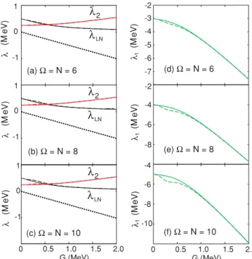
which is obtained from Eq. (23) and shown as a dashed line in Fig.1, deviates from its quasiparticle mean-field value−G/2 already atG=0 because the quantityα≡4λ2−G=0 even atG=0 (orλ2 =0 even at=0). This deviation increases withG. As has been analyzed in Ref. [2], this discrepancy is caused by the admixture of the four-quasiparticle components in the ground state from the omission of the term∼(α†)4 of
the trial Hamiltonian. Consequently, the energy shiftELNof the ground state obtained within the LN method at very small
Gdoes not coincide with the prediction by the perturbation theory. However, this discrepancy vanishes after adding the four-quasiparticle contribution toELN.
We also calculated the exact values of parametersλ2from
Eq. (27), andλ1from Eq. (25) by using the exact free energy
FLN, which is obtained from the exactELNgiven by Eq. (26)
with the entropy equal to zero atT =0. From them the exact
λLNis found by using Eq. (23). These exact values (solid lines
in Fig.1) practically coincide with those obtained by solving the LN equations. These results demonstrate how the chemical potentialµis different from its corresponding quantity, which included the effects due to quantal fluctuations beyond the quasiparticle mean field.
B. Chemical potentials within and beyond quasiparticle mean field atT=0
The chemical potentialµof the Richardson model (equal to
λin the quasiparticle mean field) becomes a constant, which remains in the middle of the single-particle spectrum (i.e., zero in the present choice ofj) only in the half-filled case
-1 0 1
-1 0 1
-1 0 1
0 0.5 1.0 1.5 2.0 G (MeV)
-7 -6 -5 -4 -3 -2
-8 -6 -4 -2
-10 -8 -6 -4
0 0.5 1.0 1.5 2.0 G (MeV)
(M
eV)
λ
(M
eV)
λ
(M
eV)
λ
(M
eV)
λ
(M
eV)
λ
(M
eV)
λ
1
1
1
(a) Ω = N = 6
(b) Ω = N = 8
(c) Ω = N = 10
(d) Ω = N = 6
(e) Ω = N = 8
(f) Ω = N = 10 λ2
λLN
λ2 λLN
λ2 λLN
FIG. 1. (Color online) Chemical potentialλLN, the parametersλ2
[(a)–(c)], andλ1[(d)–(f)] as functions of pairing interaction parameter
GatT =0 for=N=6, 8, and 10. The solid and dashed lines are
the exact and LN results, respectively, whereas the dotted lines show
the−G/2 values.
that neglects the self-energy corrections−Gvj2in the single-particle energiesj (19). In all other cases, where=N, the chemical potentialµdepends on temperatureT, no matter the self-energy corrections−Gv2
j are included or not. The values
of µobtained within the BCS theory are shown in Fig.2as functions ofT for the underfilled cases with=11,N =10, atG=0.4 MeV, and=12,N =8, atG=0.6 MeV along with the exact GCE and CE results. To be compared with the BCS results obtained without the self-energy corrections, the exact GCE (CE) results are calculated by using the exact GCE (CE) total energy shifted by−Gjf2
j, wherefjare the exact
single-particle occupation numbers obtained within the GCE (CE) (see the thin solid lines in Fig.2). The BCS chemical
ε' = j ε - G vj j 2
ε' = j εj
0 2 4 6 8 10
T (MeV)
Ω = 11, N = 10 G = 0.4 MeV
(a)
-0.4
-0.8
-1.2
-1.4 0
-5 -4 -3 -2 -1 0
0 2 4 6 8 10
T (MeV)
Ω = 12, N = 8 G = 0.6 MeV
(b)
thin thick
µ
(MeV)
µ
(MeV)
-6
exact GCE exact CE BCS
FIG. 2. (Color online) Chemical potentials as functions of
tem-peratureT for the underfilled cases with=11,N =10 (a) and
=12,N=8 (b). The dotted, solid, and dashed lines are the BCS,
exact GCE, and CE results, respectively. The thin lines denote the
BCS results obtained without the self-energy corrections−Gv2
j in
potentials decrease with increasingT atT > Tcin agreement
with the exact GCE and CE results [Eq. (2)]. Neglecting the self-energy corrections causes only a shift upward of around 0.2∼0.3 MeV. However, the BCS results, obtained including the self-energy corrections−Gv2
j, contain some small jumps
at the values of T where the chemical potential crosses the single-particle levels. These singularities lead to some small fluctuations in the valuesµ obtained in the approximations beyond the mean field such as the LN1+SCQRPA considered in the present article, and also leads to a slower convergency. For the case with=N+1=11, which we choose as an illustration below, there is no qualitative difference between the results obtained with and without the self-energy corrections up toT =6 MeV [see Fig.2(a)]. Therefore, the terms−Gv2
j
will be omitted in further calculations atT =0 for simplicity. The free energies obtained for the systems with=N+
1=11 atG=0.4 MeV and=N =50 atG=0.3 MeV are shown in Figs.3(a)and3(c)as functions ofT. They all show the general trend of decreasing with increasingT. AtT Tc
the LN1+SCQRPA offers the lowest value for the free energy, which is the closest to the exact one for =N+1=11. However, at high T, where the quantal fluctuations vanish, and the thermal fluctuations become important, the MBCS free energies turn out to be the lowest ones. In the case with
=N+1=11, the MBCS and exact results coincide atT
1.7 MeV.
Regarding the chemical potentials, one finds a clear difference between λ and µ [Eq. (2)] as functions of T as well. The thermodynamic potential µ starts from zero and decreases with increasingT in the underfilled case [Fig.3(b)],
(b)
λ, µ
(MeV)
-0.2 0.0 0.2 0.4 0.6 0.8 1.0 1.2 1.4
0 1 2 3
T (MeV)
Ω = N+1 = 11
(d)Ω = N = 50
λ, µ
(MeV)
-40 -30
BCS MBCS
exact GCE LN
-50
F (MeV)
-650 -640 -630
0 1 2 3
T (MeV)
(a)Ω = N+1 = 11
(c)Ω = N = 50
F (MeV)
LN1+SCQRPA
thin λ thick µ -0.2
0.0 0.2 0.4 0.6 0.8 1.0
thin λ thick µ
exact
λ
LN
exact CE
FIG. 3. (Color online) Free energiesF and chemical potentials
µandλas functions of temperatureT for=N+1=11 atG=
0.4 MeV (a,b) and=N= 50 (c,d) atG= 0.3 MeV. In (a) and
(c) the thin dotted, dash-dotted, and dash-double dotted lines are
the BCS, LN, and LN1+SCQRPA results, respectively. The MBCS
results are shown by the dashed lines, whereas the thick solid and thick dotted lines in (a) are the exact free energy within the GCE and CE, respectively. In (b) and (d), except for the thin solid line
representing the exactλLNas explained in the text, the other thin lines
show the chemical potentialsλobtained within the above-mentioned
approximations as notated in (a) and (c), whereas the thick lines are
the corresponding thermodynamic chemical potentialsµ.
whereas it remains temperature independent in the half-filled case with=N [Fig.3(d)]. The MBCS result with=11 and N =10 exhibits a µ, which slightly increases at T ∼
1 MeV. The reason is due to the shortcoming of the MBCS theory at lowandN, which has been discussed in a series of articles [9,10,20], and we are not going to repeat it here. Therefore, whenµis calculated within the MBCS theory by using Eq. (2) for=11 andN =10, the result can be obtained only up toT ∼1 MeV. The chemical potentialλthat includes the effects of quantal and/or thermal fluctuations beyond the quasiparticle mean field, on the contrary, is quite different from µ. The LN and LN1+SCQRPA values for λ are significantly larger than zero, and decrease with increasingT
to merge withµonly atT > Tc. The “exact”λLNis calculated
by using the same Eq. (23), whereλ2is given by Eq. (27) with the exact energyE, whereasλ1 is found from Eq. (25) with the exactELN from Eq. (26) and exact S given by Eq. (10).
This exact λLN is shown as the thin solid line in Fig. 3(b),
which decreases smoothly as T increases, and crosses zero only at T ∼ 4 MeV. The values of λ obtained within the MBCS theory show a different temperature dependence. It is zero atT =0 because PNP is not included in the MBCS theory. As T increases, the MBCS λ increases sharply up toTc, then it continues to increase (decrease) slightly with T in the case of small (large) [see Figs.3(b) and 3(d)]. Similar to the chemical potentialλLNdefined beyond the BCS quasiparticle mean field, the quantityλobtained by solving the MBCS equations loses its meaning as the thermodynamic chemical potential µ because it includes the effects due to QNF. In this sense, within the MBCS theory, only the quantity
µ, which is shown as the thick dash lines in Figs.3(b)and3(d), corresponds to a strict thermodynamic chemical potential.
C. Chemical potentials and the onset of BEC in finite systems
Following the discussion in Sec. II C for the numerical calculations regarding the BCS-BEC transition, we choose the single-particle energiesj =j−1 withj =1, . . . , (MeV),
that is, all the levels have positive energies, except the lowest one,1=0, with bothN andbeing even numbers (N
2). At small N and, the mean-field chemical potential
λ can increase or decrease with increasing G depending on whether the model is overfilled (N > ), half-filled (N =), or underfilled (N < ). This can be easily seen
-5 0 5 10 15 20
0 1 2 3 4 5 G (MeV)
N = 16
N = 12
N = 8 = 12
Ω
µ(MeV)
T = 0
(a)
-2 -1 0 1 2 3 4
0 0.5 1 1.5 2 2.5 3 G (MeV)
EXACT BCS LN1+SCQRPA
µ
(MeV)
(b)
T = 0
Ω = 12, N = 8
FIG. 4. (Color online) (a) Chemical potentialµwithin the BCS
theory as a function of G for =12 and N= 8, 12, and 16.
(b) Chemical potential as a function ofGfor the underfilled system
with=12 andN=8. The dotted, dashed, and solid lines are the
in the simplest illustration using the seniority model with one single 2-folded level, whose eigenvalue is given as a function of senioritysas [21]
Es(N, )= − G
4
s2
−2(s−N)
1+ 1
−N2
.
(42) The chemical potentialµsen.(T =0) atT =0, according to
Eq. (2), is
µs=0(T =0)=
∂Es=0(N, )
∂N = −
G
2(−N+1). (43) This result for µ, which is obtained as the derivative of the free energy (or total energy atT =0) over the particle numberN, is the same as the prediction by the approximation Eq. (5) becauseEs(N, ) is a quadratic function ofN in the
present case, whereasS(T =0)=0. This chemical potential is negative ifN , and positive ifN > because bothN
andare even. Consequently, asGincreases, the chemical potential will decrease in the underfilled and half-filled cases, and increase in the overfilled case. The physics here is related to the behavior of the pairing gap in a small shell, which is equal to =G√N(−N/2)/2 [21]. This gap is zero for the empty (N = 0) and completely filled shells (N =2), and maximum when the shell is half-filled (N =). If the configuration space is very large or infinite, whereas N
is small, the model is always strongly underfilled (N ), so the chemical potential always decreases with increasing
G. This is the situation of infinite-size systems because the upper limit of k in the kinetic energy k2/2m is very high
or infinite, whereas the number of particles is finite. In the opposite case, if the model is overfilled (N > ), we can never get BEC (i.e., structureless bosons from the pairs of fermions) by increasing the coupling strengthGbecause the chemical potential will never reach the bottom of the spectrum, being always increasing withG. This observation is confirmed by the results for the chemical potentialµ, which are obtained within the multilevel model with =12 and N =8, 12, and 16,
and displayed in Fig.4(a). This figure shows thatµdecreases with increasingGonly forN , and the stronger the model is underfilled, the steeper the decrease of µ one gets as G
increases. The chemical potential µis a smooth function of
G, as Figs. 4(a)and4(b)demonstrate. Moreover, the results displayed in Fig.4(b)show that the LN1+SCQRPA and exact results coincide, and µ crosses zero at GBECc 2.4 MeV, signalizing the appearance of the BEC as a single quantum state. The BCS prediction slightly overestimates the exact and LN1+SCQRPA results, crossing zero atGBEC
c 2.65 MeV.
As has been mentioned in Sec.II C, a negative value ofµ
is considered as the signature of the BCS-BEC transition in infinite systems. We have shown above that a similar behavior ofµalso takes place in the finite underfilled system at large
G. However, whether this still remains the signature of the BCS-BEC transition in finite systems is not straightforward. In Fig.5, we show the ground-state energies (at T =0) and the total energies (at T = 0) as functions of the particle number N at G=10 MeV. It is seen from this figure that, in the strong coupling regime, the multilevel model under consideration becomes very similar to the seniority model, in the sense that the level distance can be neglected in first-order approximation. From Eq. (42) it follows that only atN
(i.e., the low-density limit or diluted systems), the binding energy of the ground state (i.e., the ground-state energy of the system taken with the reverse sign) approaches the limit equal to the binding energy of just one pair multiplied by the number
NP =N/2 of pairs. In this limit, the condensate of N/2
noninteracting fermion pairs, whose binding energy is G
per pair, becomes a condensation ofNB=N/2 bosons (i.e.,
a BEC). This trend can be clearly seen in Figs.5(a)and5(b), which shows that, as the ratioN/ decreases on one hand, and
increases on the other hand, the BCS, LN1+SCQRPA, and exact ground-state energies become closer to the BEC limit. We also notice that the LN1+SCQRPA results practically coalesce with the exact ones at allN. AtT Tc/2 the pairing
gap decreases only slightly as compared with the gap at
T = 0, so the picture remains nearly the same for the total
(a) Ω = 12 T = 0
g.s
(MeV)
(b) Ω=20 T = 0
-500 -450 -400 -350 -300 -250 -200 -150 -100
-500 -400 -300 -200 -100 0
(c) Ω = 12 T = T /2c
(d) Ω = 12 T = Tc
0 1 2 3 4 5 6 7 8 9 10
N 0 1 2 3 4 N5 6 7 8 9 10
Exact BEC limit BCS LN1+SCQRPA
(MeV)
-800 -700 -600 -500 -400 -300 -200 -100
-450 -400 -350 -300 -250 -200 -150 -100
FIG. 5. (Color online) (a) Ground-state energies versus the particle number
N for= 10 atG=10 MeV. (b) The
same as (a) for=20. (c) Total energies
versus N for = 12 at G= 10 MeV
atT =TBCS
c /2. (d) The same as (c) at
T =TBCS
c . The notations for the results
energies up toT Tc/2 [see Fig.5(c)]. However, atT Tc,
where the BCS gap vanishes whereas the LN1+SCQRPA and exact gaps become rather small, the total energies strongly deviate from the BEC limit. As shown in Fig.5(d), the total energies predicted by the exact results and the LN1+SCQRPA theory atT =Tcare much larger than the BEC limit, especially
at larger N, whereas the total energy predicted by the BCS theory even turns positive at N 4. Meanwhile, the total energy in the BEC limit increases only slightly by 10 MeV at
N =8.3 This example demonstrates that, even if the system reaches the BEC in the strong coupling regime at T = 0, increasing T destroys the superfluid pairing correlations. As the result, at T Tc even the lightest system can no longer
stay in the BEC regime.
IV. CONCLUSIONS
The present article studies the effects due to quantal and thermal fluctuations beyond the BCS quasiparticle mean field on the chemical potential within a model, which consists of
N particles distributed amongstdoubly folded equidistant levels interacting via a pairing force with parameter G. The results obtained at zero and finite temperatures T within several approaches such as the BCS, LN, LN1+SCQRPA, and MBCS theories are compared with the exact results, whenever the latter are available. The analysis of the numerical results show that, in general, the chemical potential of the equidistant multilevel pairing model depends on the parameter
3The results obtained within the BCS and LN1+SCQRPA theories
including the self-energy term in the single-particle energies, and the exact results obtained without subtracting the corresponding term −Gkf2
k are only slightly smaller than those shown in Fig.5. The
largest difference, seen atN =8, does not exceed 5%.
of the pairing interaction and temperature. It remains a constant in the middle of the spectrum only in the half-filled case within the mean-field approximation that neglects the self-energy corrections to the single-particle energies. Beyond the quasiparticle mean field, quantal and thermal fluctuations significantly alter the chemical potential as a function ofG
and/orT. As the result, the quantity that corresponds to the chemical potential but includes the effects due to PNF or QNF, such as the parameterλLNwithin the LN method orλwithin
the MBCS theory, gradually loses its strict physical meaning as a chemical potential with increasingT, and as the approximate PNP approach the exact one, where all PNPs are eliminated.
In the study of the chemical potential as a measure to search for the onset of BCS-BEC transition in finite systems, we have shown that the system in the strong coupling regime can approach the BEC limit only in the strongly underfilled case (when the number N of particles is much smaller than the size, that is, number of the levels of the system) at zero temperature. Even if it can take place, increasing temperature will drive the system out of the BEC limit. However, this is a conclusion obtained here within a simple one-dimensional model. How this feature is modified in realistic nuclei remains a question to be answered in the future studies.
ACKNOWLEDGMENTS
The authors thank Peter Schuck (IPN Orsay) for proposing the application to BCS-BEC transition and fruitful discus-sions. The numerical calculations were carried out using the FORTRAN IMSL Library by Visual Numerics on the RIKEN Integrated Combined Cluster (RICC) system. N.Q.H. acknowledges support from the Nishina Memorial program at RIKEN Nishina Center. He also thanks the Vietnam Na-tional Foundation for Science and Technology Development (NAFOSTED) for support through Grant No. 103.04.54.09, under which a part of this work was carried out.
[1] A. L. Goodman, Phys. Rev. C29, 1887 (1984).
[2] H. J. Lipkin, Ann. Phys.9, 272 (1960); Y. Nogami, Phys. Rev.
134, B313 (1964); H. C. Pradhan, Y. Nogami, and J. Law, Nucl.
Phys.A201, 357 (1973); J. F. Goodfellow and Y. Nogami, Can.
J. Phys.44, 1321 (1966).
[3] H. Olofsson, R. Bengtsson, and P. M¨oller, Nucl. Phys.A784,
104 (2007).
[4] N. Q. Hung and N. D. Dang, Phys. Rev. C76, 054302 (2007).
[5] L. G. Moretto, Nucl. Phys.A182, 641 (1972).
[6] A. L. Goodman, Phys. Rev. C29, 1887 (1984).
[7] N. Dinh Dang and N. Zuy Thang, J. Phys. G14, 1471 (1988).
[8] N. D. Dang, P. Ring, and R. Rossignoli, Phys. Rev. C47, 606
(1993); R. Rossignoli, P. Ring, and N. D. Dang, Phys. Lett.
B297, 9 (1992).
[9] N. Dinh Dang and V. Zelevinsky, Phys. Rev. C 64, 064319
(2001);65, 069903(E) (2002); N. Dinh Dang and A. Arima,
ibid.67, 014304, (2003);68, 039902(E) (2003); N. D. Dang and
A. Arima,ibid.74, 059801 (2006); N. Dinh Dang, Nucl. Phys.
A784, 147 (2007); N. D. Dang, Phys. Rev. C76, 064320 (2007).
[10] N. D. Dang and A. Arima, Phys. Rev. C68, 014318 (2003).
[11] P. Nozi`eres and S. Schmitt-Rink, J. Low Temp. Phys.59, 195
(1985).
[12] A. Volya, B. A. Brown, and V. Zelevinsky, Phys. Lett.B509, 37
(2001).
[13] N. Q. Hung and N. D. Dang, Phys. Rev. C79, 054328 (2009).
[14] A. Bohr and B. Mottelson,Nuclear Structure, Vol. 1 (Benjamin,
New York, 1969).
[15] N. Dinh Dang and N. Quang Hung, Phys. Rev. C77, 064315
(2008).
[16] P.-G. Reinhard, W. Nazarewicz, M. Bender, and J. A. Maruhn,
Phys. Rev. C53, 2776 (1996); T. R. Rodriguez, J. L. Egido,
and L. M. Robledo,ibid.72, 064303 (2005); M. V. Stoitsov,
J. Dobaczewski, R. Kirchner, W. Nazarewicz, and J. Terasaki,
ibid. 76, 014308 (2007); G. F. Bertsch, C. A. Bertulani,
W. Nazarewicz, N. Schunck, and M. V. Stoitsov,ibid.79, 034306
(2009).
[17] N. Dinh Dang, Z. Phys. A335, 253 (1990).
[18] N. Q. Hung and N. D. Dang, Phys. Rev. C 78, 064315
(2008).
[19] N. Dinh Dang, Eur. Phys. A16, 181 (2003).
[20] V. Yu. Ponomarev and A. I. Vdovin, Phys. Rev. C72, 034309
(2005);74, 059802 (2006)
[21] P. Ring and P. Schuck, The Nuclear Many-Body Problem