Estimation Methods for Data Subject to Detection Limits

(1)

Estimation Methods for Data Subject to Detection Limits

Ryan C. May

A dissertation submitted to the faculty of the University of North Carolina at Chapel Hill in partial fulfillment of the requirements for the degree of Doctor of Philosophy in the Department of Biostatistics.

Chapel Hill 2012

Approved by:

Dr. Joseph G. Ibrahim

Dr. Haitao Chu

Dr. Stephen Cole

Dr. Pei Fen Kuan

(2)

c

2012

Ryan C. May

(3)

Abstract

RYAN C. MAY: Estimation Methods for Data Subject to Detection Limits (Under the direction of Dr. Joseph G. Ibrahim and Dr. Haitao Chu)

(4)

(5)

Acknowledgments

I would first like to thank both of my advisors, Dr. Joseph Ibrahim and Dr. Haitao Chu, for their guidance with this work. Their immense knowlege and assistance has been a tremendous help to me, and I greatly appreciate the amount of time and effort they committed to helping me with this project.

I would also like to thank Dr. Stephen Cole, Dr. Pei Fen Kuan, and Dr. John Preisser for serving on my committee. I greatly appreciate the time they have given, and their insightful

comments have significantly (p<.05) improved the quality of this work.

I would like to also thank my fellow classmates for their friendship and help through these many years at UNC. In particular, I would like to thank Allison Deal, Annie Green Howard, Dave Kessler, Dustin Long, Leann Long, Virginia Pate, Shangbang Rao, and Vonn Walter.

Many thanks to my parents, Jeff and Ann May, for their unwavering support of a son who wants to spend 11+ years of his life in college.

(6)

List of Tables

1.1 Parameter estimates for simulation study, comparing change-point model to

linear standard deviation model and constant standard deviation model . . . 10

1.2 Parameter estimates for HIV study, using regression models and mixed models 16

2.1 Parameter estimates and standard errors, comparing EM algorithm approach

to complete-case analysis and substitution of LOD/√2. 1000 Datasets were

used for each analysis, with 250 samples taken for each observation below the

limit of detection. . . 31

2.2 Logistic regression model summary for NHANES data, comparing maximum

likelihood approach to complete case analysis and ad-hoc substitution of LOD/√2 36

(9)

List of Figures

1.1 Plot of raw data from six experiments in the HIV study . . . 14

1.2 Change-point model results for experiments 1 and 3 . . . 15

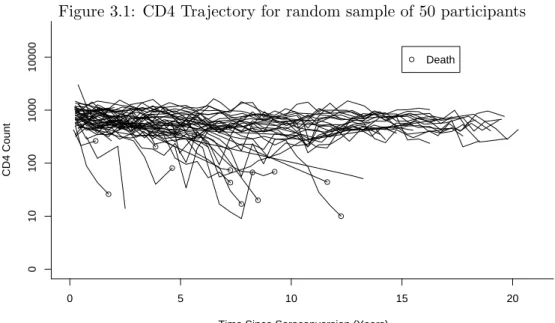
3.1 CD4 Trajectory for random sample of 50 participants . . . 45

(10)

List of Abbreviations

• ARMS - Adaptive Rejection Metropolis Sampling

• HIV - Human Immunodeficiency Virus

• LOD - Limit of Detection

• LOQ - Limit of Quantitation

• MLE - Maximum Likelihood Estimate

• MACS - Multicenter AIDS Cohort Study

(11)

Chapter 1 Change-Point Models to Estimate the

Limit of Detection

1.1 Introduction

In many laboratory assays, interest resides in quantifying very dilute quantities in solution. As concentrations of analytes decrease, however, the resulting measured levels from a mea-surement device often become less precise. At some low concentration level, a measured response cannot accurately be distinguished from background noise, the measured response from a blank sample. This low concentration point is called the limit of detection (LOD), a point that is specific to each particular measurement device (Clinical and Laboratory Stan-dards Institute, 2004). Though the general definition given above for the limit of detection is widely accepted, the methodology used to determine the limit of detection is quite varied. In this chapter we consider the estimation of the limit of detection using repeated measurements from known analyte concentrations. This analysis is motivated by data from a study of low levels of HIV that persist despite potent therapy, in which a novel assay was developed to detect changes in low-level HIV expression after a drug intervention. The assay measuring HIV expression becomes less precise as the concentration of HIV decreases, but a limit of detection for the assay is not known. In this chapter we consider estimating the LOD for this assay based on measurements replicated on several solutions containing known quantities of HIV.

(12)

the proposed change-point model and discuss a two-stage estimation approach for obtaining maximum likelihood estimates from the model. In Section 1.4, we examine the proposed model using a simulation study, then apply the method to data from the aforementioned HIV assay in Section 1.5. We conclude this chapter in Section 1.6 with a discussion.

1.2 Background

To distinguish between low analyte concentrations and those of a blank sample, many esti-mation approaches aim to quantify the distribution of measurements obtained from a blank sample. The distribution of assay measurements for a blank sample is often assumed to be

Gaussian, with meanµblank and varianceσ2_blank (Anderson 1989). A limit of detection is then

chosen to fall a “reasonable” distance outside of this blank distribution. Consequently, many definitions of LOD take the following form (Whitcomb and Schisterman 2008):

LOD =µblank+Kσblank (1.1)

where K is a definition-specific constant, usually in the range of 2.0 to 3.0 (Browne and

Whitcomb 2010, Long and Winefordner 1983, Thomsen et al. 2003).

When K = 3, it is expected that 99.9% of measurements from a blank sample will fall

below the limit of detection. Clearly, the larger value ofK that is chosen, the higher the LOD

will be, and the lower the chance that a value from a blank will fall above the LOD. Using

this definition, many estimation approaches are designed to accurately estimate µblank and

σblank. In practice, such estimation is straightforward when many repeated measurements

can be obtained from a blank sample, by taking the sample mean and standard deviation

(SD) as estimates ofµblank and σblank.

When blank measurements are not available, alternative estimation approaches can be utilized. One approach involves taking repeated measurements of a known low concentration of analyte and using these measurements as proxy measurements for a blank sample. In this

case, the LOD definition is extremely similar to (1.1). Withµlow and σlow representing the

(13)

(again assumed to follow a Gaussian distribution), the limit of detection is defined as:

LOD =µlow+Kσlow (1.2)

The previous definition of the LOD in (1.1) includes only a specification of the distribution of a blank sample. Using this definition enables direct control of the type I error, the chance of incorrectly specifying a blank sample as containing some concentration of analyte. For

example, when K = 3 the chance of a type I error is only 0.1% for any particular blank

measurement. However, this specification does not control for type II error, the chance of incorrectly specifying a sample containing analyte as coming from a blank. If the type II error is high, clearly there is still difficulty in conclusively distinguishing a concentration value near the LOD from a blank. Consequently, many definitions of the LOD take both type I and type II error into account. To ensure that measured values for concentrations at the LOD are unlikely to fall in the range of a blank sample, alternative definitions of LOD account for the distribution of measurement values at some known small concentration of analyte. The limit of detection is defined as follows (Armbruster and Pry 2008, Browne and Whitcomb 2010):

LOD =µblank+ 1.645σblank+ 1.645σlow (1.3)

Using this definition, 95% of blank samples will fall below µblank+ 1.645σblank (called the

“limit of blank”, or “limit of decision”), and 95% of measurements for concentrations at the limit of detection will fall above the limit of blank. It should be noted that definition (1.3) is only needed when it is assumed that the measurement standard deviation for a blank sample is different from the standard deviation for any other “low” concentration sample at or around

the LOD (i.e. σblank 6=σlow). Many authors (Anderson 1989, Armbruster 1994, Browne and

Whitcomb 2010) assume a constant measurement error variance for any true concentrations

near or below the limit of detection. In this case, the choice ofK in (1.1) specifies the chance

of a type I or type II error. When K = 3.29, the chance of either type of misclassification is

5%; whenK = 3, the chance is 7%. Alternative (but similar) definitions to (1.3) calculate a

(14)

estimate in place of bothσblank and σlow (Long and Winefordner 1982).

The LOD definitions displayed in equations (1.1) and (1.3) usually are performed under the assumption that the measurement distribution for a blank sample is Gaussian. In reality, characteristics of the measurement device often result in non-Gaussian measurement distri-butions for a blank. In such cases, nonparametric methods have been proposed (Linnet and Kondratovich 2004), which involve estimating quantiles from the observed blank distribution.

For definition (1.3), the value of σlow can still be estimated with parametric methods when

it is reasonable to assume a Gaussian distribution for a low concentration sample. If the low

concentration cannot be assumed Gaussian, quantile estimation can be used to estimateσlow

as well.

In practice, data analysts often do not have access to replicates of data from blank or “low” concentrations. This is the case for the HIV pilot study data considered in Section 1.5, in which the number of polymerase chain reaction (PCR) cycles needed to obtain a blank sample measurement is too high to be operationally feasible. In this case it is difficult to directly estimate the distribution of measurements for a blank sample, or for the distribution of any low concentration sample. Estimation often proceeds using higher analyte concen-trations from which measurements are more easily obtained. A regression line is then fit to (X1, Y1), ...,(Xn, Yn), the n observed pairs of analyte concentrations X and measured

re-sponses Y. This fitted regression line is known as a linear calibration curve. Assuming a

linear relationship betweenXandY, we have the following model specification (Dunne 1995,

Hubaux and Vos 1970):

Yi =β0+β1Xi+i, i ∼N(0, σ2) (1.4)

Taking θ = (β0, β1, σ2), the assumptions of (1.4) specify the distribution of Yi|Xi,θ ∼

N(β0 +β1Xi, σ2). Clearly, the parameter estimates of the model can be used to directly

estimate the distribution of YXi=0, the response for a blank sample. When the parameter

vectorθ is known, we have:

YXi=0|θ∼N(β0, σ

(15)

Using the definition of LOD in equation (1.1) withK = 3, the LOD under model (1.4) is:

LODY =β0+ 3σ

The above specification is conditional on the true values of the model parameters β0,β1,

andσ2. Let ˆβ0, ˆβ1, and ˆσ2 denote the Maximum Likelihood Estimates (MLE’s) forβ0,β1, and

σ2 (and denoteV[ ˆβ0] = ˆσ_β2₀). The response distribution for a blank sample can be estimated

as follows:

YXi=0∼N( ˆβ0,σˆ

2_{+ ˆ}_σ2

β0)

Consequently, the limit of detection can be estimated as (Cox 2005, Hubaux and Vos 1970):

[

LODY = ˆβ0+ 3(ˆσ2+ ˆσβ20)

1/2 _(1.5)

In practice, the limit of detection is usually defined in terms of the concentrationXinstead

of the measurement Y. To obtain the limit of detection for concentration, a simple linear

transformation onLOD[Y is performed (Gibbons et al., 1992), to obtain:

[

LODX =

3(ˆσ2+ ˆσ2_β 0)

1/2

ˆ

β1

(1.6)

The standard analysis for estimating the LOD with a linear calibration curve assumes that the variance of measured responses is constant at all concentration values. In many practical applications this is not the case, and it is common for a measurement device to become more (or less) precise as the concentration of analyte increases. In the most basic case (or possibly under suitable transformation), the measurement standard deviation is assumed to decrease linearly with the concentration. This case was first considered by Oppenheimer et al. (1983), and specifies the error distribution from model (1.4) as follows:

i ∼N(0,(σ0+σ1Xi)2) (1.7)

(16)

equations (1.5) and (1.6).

Current analysis methods for estimating the limit of detection with a linear calibration curve either assume a constant standard deviation for measurement error as in (1.4), or a linear change in measurement standard deviation by concentration as in (1.7). As noted by several authors (Armbruster 1994, Hubaux and Vos 1970, Clinical and Laboratory Standards Institute 2004, Browne and Whitcomb 2010), a more realistic assumption is that the measure-ment standard deviation changes for “high” concentration values above the limit of detection, while remaining effectively constant for “low” concentration values. Under this assumption, the use of a constant standard deviation model like (1.4) for all concentration values can result in underestimation (if precision increases with concentration) or overestimation (if precision decreases with concentration) of the limit of detection. The use of a linear standard deviation model like (1.7) could provide the opposite effect, overestimating the LOD when precision in-creases with concentration and underestimating when precision dein-creases with concentration. To correct these potential biases in LOD estimation with a linear calibration curve, in Section 1.3 a change-point model is proposed to more accurately model the measurement error for all concentrations.

1.3 Change-Point Model

In Section 1.2 it was discussed that current analyses using a linear calibration curve usually assume either a constant measurement standard deviation for all analyte concentrations, or a measurement standard deviation that varies linearly with the analyte concentration. Because measurements below the limit of detection are indistinguishable from a blank, it follows that the measurement standard deviation should be constant for low analyte concentrations. Such a distribution can be modeled using a change-point for the measurement standard deviation. While the literature on change-point models in both regression (Bai 1997, Hawkins 2001) and mixed (Cudeck and Klebe 2002) modeling is quite rich, to our knowledge no published articles have looked at models with a change-point on the standard deviation of the error. Taking

(17)

the measurement standard deviation for concentrationXi, we make the following assumption

for the form ofσi:

σi =



  

  

σ0 ifXi ≤λ

σ0+σ1(Xi−λ) ifXi > λ

(1.8)

whereλrepresents the change-point for measurement standard deviation. As noted in Section

1.2, a common definition for the LOD is 3 standard deviations away from the expected value of a blank sample. Given the assumption in equation (1.8), the standard deviation of a blank

sample isσ0. The expected value of the blank sample is the intercept term for the model,β0.

The LOD for both the measurement (Y) and true concentration (X) are:

LODY =β0+ 3σ0 (1.9)

LODX =

3σ0

β1

(1.10)

Taking ˆβ0, ˆσ0, ˆσβ0, and ˆβ1 as the MLE’s for their respective parameters, the limit of

detection is estimated following equations (1.5) and (1.6):

[

LODY = ˆβ0+ 3(ˆσ20+ ˆσ2β0)

1/2

[

LODX =

3(ˆσ₀2+ ˆσ_β2₀)1/2 ˆ

β1

(1.11)

In the situation described above, the MLE’s ˆβ0, ˆβ1, and ˆσ have a simple closed form.

However, in the HIV pilot study motivating this work the measured assay responses Y are

right-censored at a constant upper limit (here denoted as γ). Accounting for this censoring,

the log-likelihood for an individual observation is:

li=



  

  

−log(σi)−₂_σ12

i

(Yi−(β0+β1Xi))2 ifYi ≤γ

log

h

1−Φ

n

γ−(β0+β1Xi)

σi

oi

ifYi > γ

(18)

Again denoting (X1, Y1), ...,(Xn, Yn) as the n iid observations available for analysis, the

log-likelihood for the model can be expressed as:

l(β0, β1, σ0, σ1, λ) =

n

X

i=1

li (1.12)

In order to estimate the LOD under model 1.8, we maximize the log-likelihood (1.12) with

respect to the parameter vector (β0, β1, σ0, σ1, λ). Maximization of the log-likelihood is done

under the following constraints. First, the change-point (λ) must be constrained within the

range of the observedXi. Takingx(1)...x(n) as the order statistics for the observedXi, this is

expressed asx(1)≤λ≤x(n). The rationale for this constraint is that the parameters σ0 and

λbecome unidentifiable when λ≤x(1), and the parametersσ1 and λbecome unidentifiable

whenλ≥x(n).

The second model constraint is that the error standard deviation σi cannot be negative

atx₍₁₎, and the third model constraint is thatσi cannot be negative atx(n). Together, these

constraints specify thatσi is nonnegative at all points in [x(1), x(n)]. One way to specify these

constraints is to require σ0 ≥0 and σ0+σ1(x(n)−λ) ≥0. All constraints on the model are

given below:

(i) x(1) ≤λ≤x(n)

(ii) σ0 ≥0

(iii) σ0+σ1(x(n)−λ)≥0

Constraints (i) and (ii) are both linear, so are straightforward to implement in any maxi-mization of the resulting log-likelihood. However, constraint (iii) is not linear, as it involves

the term σ1λ. Therefore, maximizing (1.12) subject to (i), (ii), and (iii) is challenging since

many standard optimization routines only allow for linear constraints. To get around this issue, we instead use a two-stage optimization routine (Smyth 1996). For ease of exposition,

we will defineσx(n) =σ0+σ1(x(n)−λ), the standard deviation atx(n), the maximum observed

(19)

thet-th iteration of the estimation routine. The proposed two-stage optimization routine is as follows:

1. Fixλ=λ(t−1). Maximize (1.12) with fixed λ, subject to thelinear constraints:

i) σ0 ≥0

ii) σ0+σ1(x(n)−λ)≥0

2. Taking ˆσ0 and ˆσ1 as the estimates from step 1, fix σx(n) = ˆσ0 + ˆσ1(x(n) −λ

(t−1)_).

Maximize (1.12) with fixedσx(n) subject to thelinear constraints:

i) x₍₁₎ ≤λ≤x₍_n₎

ii) σ0 ≥0

Obtain estimatesβ₀(t),β₁(t),σ₀(t),λ(t), setσ₁(t)= (σx(n) −σ

(t)

0 )/(x(n)−λ(t))

Steps 1 and 2 in the above procedure are repeated until convergence is achieved for all

parameter estimates. The convergence criterion used for parameter φ specifies that φ(t) ₋

φ(t−1)≤K, withKagain representing a generic constant. The proposed optimization routine

is relatively simple to implement, as the likelihood in (1.12) is not overly complex. For

all individual model analyses presented in Sections 1.4 and 1.5, optimization in each stage

was performed using R software (R Development Core Team 2008) with the constrOptim()

function. In the following section we perform a simulation study to test the new estimation approach, and then apply our approach to data from an HIV pilot study.

1.4 Simulation Study

A simulation study was conducted to analyze the performance of the proposed change-point model. The data for this simulation study was generated using a parameter specification that mirrored that for the HIV data analysis presented in Section 1.5. The model was specified as:

(20)

(21)

withσi having the change-point specification given by (1.8).

Following the HIV data, only 5 different values of concentration Xi were used at 1, 2,

3, 4, and 5. For each of the concentration values used, repeated measurements (Yi) were

generated. The number of Yi generated for each of the 5 concentration values was equal,

a balanced allocation. For all simulations, the parameter values were specified as follows:

β0 = 45, β1 = −3.7, σ0 = 1.1. Four different sets of simulations were run using a different

value for the change-point, withλtaking values 1.5, 2.5, 3.5, and 4.5 to span the range ofXi.

The value of σX(n), the standard deviation at the maximum concentration value, was kept

constant at 0.25 for all simulations (again mirroring results from the HIV data analysis). The

specified values ofσ0, λ, andσX(n) determined the parameter value of σ1 for each simulated

data set. Following the real-life data set in Section 1.5, all values ofYi falling above 42 were

set as right-censored.

For each simulation scenario, 10,000 data sets of size 80, 150, and 300 were generated. The proposed change-point model was then fit to the data, using the two-stage estimation approach to obtain maximum likelihood estimates of all the model parameters. For comparison, model (1.7) assuming a linear change in standard deviation with no change-point and model (1.4) assuming constant standard deviation were also fit to the simulated data sets.

(22)

In addition to parameter estimates, the Akaike Information Criterion (AIC, Akaike 1974) was also calculated for each of the three models fit to every simulated data set. For each set of 10,000 simulated data sets, the model with the lowest AIC was selected as the best fit for the current data set. Table 1.1 displays the proportion of simulated data sets that

resulted in a particular model having the best fit. For example, with N = 80 andλ= 4.5, the

change-point model had the best model fit in 96.0% of the simulated data sets, compared to 0.6% for the linear standard deviation model and 3.4% for the constant standard deviation model. The results displayed in table 1.1 show that the change-point model produces the best fit to the data a much higher proportion of the time than either the linear standard deviation or constant standard deviation models, for all simulation scenarios. This “relative fit” of the change-point model increased with increasing change point, and also with sample size, from

60.3% in the N = 80,λ= 1.5 simulation to 100% in the N = 300,λ= 4.5 simulation.

1.5 HIV Data

Data for this analysis comes from an HIV pilot study analyzing the effects of a drug on HIV transcription. Resting cells from HIV infected patients are treated with the drug, with interest in the degree to which HIV transcription is increased. HIV RNA in general is too unstable and must be reverse transcribed into the more stable form, cDNA. The concentration of HIV RNA in patient samples is much too low to be directly measured, and following conversion to cDNA subsequent amplification by quantitative PCR is necessary (Nolan et al. 2006, Palmer et al. 2003). The region of the HIV genome amplified in this assay codes for a highly

conservative region known as gag which is measured with primers and probes as described

(23)

concentration can be estimated.

For each patient in the pilot study, a linear calibration curve is created by measuring

the cycle-threshold value for different known dilutions of HIV. Data for the study consists

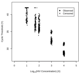
of calibration curve data for six experiments (one for each patient), with each experiment consisting of 20 measurements for each of 4-5 known concentrations of HIV. The goal of the analysis is to estimate the limit of detection for the concentration of HIV individually for each experiment. Complicating the analysis is the restriction that each sample was run for a maximum of 42 cycles of PCR amplification; HIV concentrations resulting in more than 42 cycles are right-censored. A plot of the raw data for all six experiments is presented in Figure 1.1.

It is important to note here that the concentration of HIV (X) is inversely related to the cycle-threshold value (Y) in the analyzed data. A lower concentration of HIV will take more PCR cycles to fluoresce, resulting in a higher cycle-threshold value. This relationship is the opposite of what is usually observed when relating known concentrations to measured values, where measurement (Y) usually increases with analyte concentration (X). Because of

the inverse relationship between Y and X in the current data, the LOD estimates will be

slightly altered from (1.13), taking the form:

[

LODY = ˆβ0−3(ˆσ20+ ˆσ2β0)

1/2

[

LODX =

−3(ˆσ2₀+ ˆσ2_β

0)

1/2

ˆ

β1

(1.13)

Analysis of the data was performed in two ways. First, the change-point model proposed in Section 1.3 was fitted separately for each individual experiment, generating experiment-specific LOD estimates. Additionally, a mixed-model approach was also considered. The mixed model allows for simultaneous estimation of the LOD for all experiments. The model specification is given as follows:

(24)

● ● ● ● ● ● ● ● ● ● ● ● ● ● ● ● ●● ● ● ● ● ● ● ● ● ● ● ●● ● ● ● ● ● ● ● ●●●● ● ● ● ● ● ● ● ● ● ● ● ● ● ● ● ● ● ● ● ● ● ● ● ● ● ● ● ● ● ● ● ● ● ● ● ● ●● ●●● ● ● ● ● ● ● ● ● ● ● ● ● ● ● ● ● ● ● ● ● ● ●● ●● ● ● ● ● ● ● ● ● ● ● ● ● ● ● ● ● ● ● ● ● ● ●● ● ● ● ● ● ● ● ● ● ● ● ● ●●● ● ● ● ● ● ● ● ● ● ● ● ●● ● ● ● ● ● ● ● ● ● ● ● ●●●● ●● ● ● ● ● ● ● ● ● ●● ● ● ● ● ● ● ●●●● ●●●● ● ● ● ● ● ● ●● ● ● ● ● ● ● ● ● ● ● ● ● ● ● ● ● ● ●● ● ● ● ● ● ● ● ● ● ● ● ● ● ● ● ● ● ●●● ● ● ● ● ● ● ● ● ● ● ● ●● ●●●● ● ● ● ● ● ● ● ● ● ● ● ● ●● ● ● ● ● ● ● ● ● ● ● ● ● ● ● ● ● ● ● ● ● ● ● ● ● ● ●● ● ● ●● ● ● ● ● ● ● ● ● ● ● ● ● ● ● ● ● ● ● ● ● ● ● ● ● ●● ● ● ● ● ● ● ● ● ● ● ● ● ● ● ● ● ● ● ● ● ● ● ● ● ● ● ● ● ● ● ● ● ● ● ● ● ● ● ● ● ●● ● ● ● ● ● ● ● ● ● ● ● ● ● ● ● ●● ● ● ● ● ● ● ● ● ● ● ● ● ● ● ● ● ● ● ● ● ● ● ● ● ● ● ● ● ● ● ● ● ● ● ● ●●● ● ●● ● ● ● ● ● ● ● ● ● ● ● ● ● ● ● ●● ● ● ● ● ● ● ● ● ● ● ● ● ● ● ● ● ● ●● ● ● ● ● ● ● ● ● ● ● ● ● ● ● ● ●● ● ● ● ● ● ● ● ● ● ● ● ● ● ●

0 1 2 3 4 5

30

35

40

Log10(HIV Concentration) (X)

Cycle Threshold (Y)

● Observed Censored

Figure 1.1: Plot of raw data from six experiments in the HIV study

σij =

      

σ0 ifXij ≤λi

σ0+σ1(Xij −λi) ifXij > λi

(bi0, bi1)∼M V N



 0,



 

σ_b2

0 ρσb0σb1 ρσb0σb1 σ

2 b1      

whereYij is the cycle-threshold value andXij is the log10concentration of HIV for experiment

i and measurement j. The abbreviation M V N denotes a multivariate normal distribution.

Maximum likelihood estimation for this model was performed using PROC NLMIXED in SAS

software version 9.3. As with the simulation study, both linear standard deviation and con-stant standard deviation models were included for comparison. The model fit was again analyzed using the AIC.

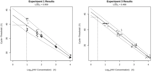
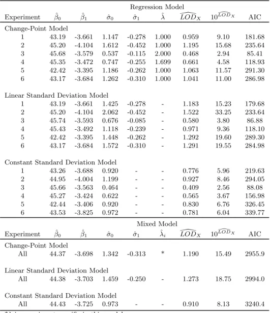
Parameter estimates for both the regression and mixed model approaches are given in Table 1.2, and a plot of the model fit for experiments 1 and 3 is given in Figure 1.2. The dashed lines about the predicted regression line in Figure 1.2 represent a 95% prediction interval for the data, with the vertical and horizontal dashed lines representing the estimated LOD.

Estimates of experiment-specific LODs (denotedLOD[X in table 1.2) using the change-point

(25)

HIV concentrations of 2.94 to 15.68 copies of gag. LOD estimates from the change-point model were lower than those from the linear standard deviation model, and were higher than estimates from the constant standard deviation model, for all experiments. Interestingly, the AIC for the change-point model was lower than the AIC for the linear standard deviation model in only one of the six experiments tested, suggesting that the linear standard deviation model generally provided a better fit to the data when the regression model was utilized. In experiments 1, 2, 5, and 6, the change-point estimates equal 1.0, the lowest observed concentration value. This makes the likelihood for the model identical to the linear standard

deviation model (notice the identical parameter estimates for β0 and β1), only with more

parameters estimated in the change-point model. This results in the higher AIC value for the change-point model.

The mixed model results also give LOD estimates for the change-point model that are higher than the constant standard deviation model, and lower than the linear standard devi-ation model. The un-logged LOD estimate of 15.49 is in the range of LOD estimates for the regression change-point models on each experiment, as expected. The AIC results indicate that the change-point model provides a better fit to the available data than does the linear standard deviation or constant standard deviation mixed models.

● ●● ● ● ● ● ● ● ● ● ● ● ● ● ● ●● ● ● ● ● ● ● ● ● ● ● ● ● ● ● ● ● ● ● ● ● ● ● ● ● ●● ● ● ● ● ● ● ● ● ● ● ● ● ● ● ● ● ● ● ● ● ● ● ●● ● ● ● ● ●● ● ● ● ● ● ●

0 1 2 3 4

30

35

40

45

Experiment 1 Results

Cycle−Threshold (Y)

LODX ^ = 0.959 ●● ● ● ● ● ● ● ● ● ● ● ● ● ● ● ● ●● ●● ●● ● ● ● ● ● ● ● ● ● ● ● ● ● ● ● ● ● ● ● ● ● ● ●● ●●● ● ● ●●● ● ● ● ● ● ●●●

0 1 2 3 4

35

40

45

Experiment 3 Results

Cycle−Threshold (Y)

LODX ^

= 0.468

(26)

Table 1.2: Parameter estimates for HIV study, using regression models and mixed models

Regression Model

Experiment βˆ0 βˆ1 σˆ0 σˆ1 ˆλ LOD\X 10LOD\X AIC

Change-Point Model

1 43.19 -3.661 1.147 -0.278 1.000 0.959 9.10 181.68

2 45.20 -4.104 1.612 -0.452 1.000 1.195 15.68 235.64

3 45.68 -3.579 0.537 -0.115 2.000 0.468 2.94 85.41

4 45.35 -3.472 0.747 -0.255 1.699 0.661 4.58 118.93

5 42.42 -3.395 1.186 -0.262 1.000 1.063 11.57 291.30

6 43.17 -3.684 1.262 -0.310 1.000 1.041 11.00 286.98

Linear Standard Deviation Model

1 43.19 -3.661 1.425 -0.278 - 1.183 15.23 179.68

2 45.20 -4.104 2.062 -0.452 - 1.522 33.25 233.64

3 45.74 -3.593 0.676 -0.085 - 0.580 3.80 86.88

4 45.43 -3.492 1.118 -0.239 - 0.971 9.36 118.10

5 42.42 -3.395 1.448 -0.262 - 1.292 19.60 289.30

6 43.17 -3.684 1.572 -0.310 - 1.291 19.55 284.98

Constant Standard Deviation Model

1 43.26 -3.688 0.920 - - 0.776 5.96 219.63

2 44.95 -4.004 1.199 - - 0.927 8.46 294.05

3 45.66 -3.563 0.464 - - 0.409 2.56 88.08

4 45.27 -3.424 0.622 - - 0.565 3.67 156.98

5 42.44 -3.406 0.920 - - 0.830 6.76 326.45

6 43.53 -3.825 0.972 - - 0.781 6.04 339.77

Mixed Model

Experiment βˆ0 βˆ1 σˆ0 σˆ1 λˆi LOD\X 10LOD\X AIC

Change-Point Model

All 44.37 -3.698 1.342 -0.313 * 1.190 15.49 2955.9

Linear Standard Deviation Model

All 44.38 -3.703 1.459 -0.250 - 1.273 18.75 2994.0

Constant Standard Deviation Model

All 44.43 -3.725 0.973 - - 0.910 8.13 3240.4

(27)

1.6 Discussion

In this chapter we have developed a change-point model to estimate the limit of detection with a linear calibration curve. In certain settings, the proposed approach may provide a more realistic modeling of the underlying distribution of measurement errors in a linear calibration curve. Estimation is performed via a two-stage estimation technique, such that the nonlinear constraints on the model parameters are satisfied. We have demonstrated application of the proposed model using both an individual regression model and a mixed model.

The simulation results presented in Table 1.1 demonstrate that the proposed change-point model can dramatically improve estimation of the limit of detection when compared to both the linear standard deviation and constant standard deviation models. When measurement error is constant for low concentrations of analyte, the linear standard deviation model tends to overestimate the measurement error for a blank sample, and consequently tends to overes-timate the limit of detection. This is shown quite dramatically in Table 1.1, where esoveres-timates using the change-point model exhibit smaller bias than the linear standard deviation model, particularly when more of the observed data falls below the true change-point. The constant standard deviation model was shown to underestimate the LOD for all simulations considered, with a significantly larger bias than the change-point model. When AIC fit statistics were analyzed, the change-point model was correctly identified as the model providing the best fit to the data, for all simulations considered.

The key assumption of the proposed change-point model is that the measurement error standard deviation is constant below some low concentration value. If this assumption does not hold (the standard deviation instead continues to increase or decrease with concentration), the change-point model would be expected to exhibit a greater bias than the linear standard deviation model. In this case, when the measurement error increases with concentration, the change-point model would tend to overestimate the limit of detection. When the measurement error decreases with concentration, the change-point model would tend to underestimate the LOD.

(28)

(29)

Chapter 2 Maximum Likelihood Estimation in

Generalized Linear Models With Multiple

Covariates Subject to Detection Limits

2.1 Introduction

While the previous chapter concerned estimation of the limit of detection itself, the current topic considers analysis of data subject to detection limits with a predetermined limit of de-tection. Specifically, we are interested in estimation with generalized linear models (GLM’s) in which multiple covariates are subject to a limit of detection. While the proposed method-ology in this chapter can be applied to both right- and left-censored covariate data, the real and simulated examples presented here consider only left-censored data, as is most common in real-life studies with detection limits. To motivate these methods, we consider a study in cancer incidence conducted within the National Health and Nutrition Examination Survey (NHANES). As part of this study, levels of urinary heavy metals were recorded, along with presence of any form of cancer. Recorded urinary heavy metals included cadmium, uranium, tungsten, and dimethylarsonic acid. The measurement device used to examine levels of each urinary heavy metal can only be calibrated down to a specific limit of detection (i.e. only above 1.7 ug/L for dimethylarsonic acid). As a result, 24.1% of the 1350 patients had at least one covariate value that fell below the limit of detection for the measurement device. Study subjects were also surveyed as to past cancer status, the response variable for this study.

Past research on data subject to detection limits has considered models where either

the response or covariates alone are subject to detection limits. The simplest and most

(30)

falling below the limit of detection. This is known as complete-case analysis. Complete-case analysis is generally discouraged because of the loss of useful information in the data. Though complete-case analysis can give unbiased parameter estimates in regression models (Rigobon and Stoker 2007, D’Angelo and Weissfeld 2008, Nie et al. 2010), the standard errors of those estimates will be inflated due to the decreased sample size. This deficiency is particularly significant for studies where a large proportion of data falls below the limit of detection. Additionally, background parameter estimates for the covariate distribution of interest will be biased (Helsel, 2005). Another very common approach is to use ad-hoc substitution methods. These often include substituting some fraction of the limit of detection for all observations falling below the limit of detection, such as the limit of detection itself

(LOD), LOD/2, LOD/√2, or zero. Such methods are commonly employed because they

are simple both to understand and implement. However, numerous authors have concluded that such methods are statistically inappropriate (see Helsel, 2006 and Lubin, 2004 for a discussion with censored responses, and Lynn, 2001 for censored covariates). Helsel (2005) provides a review of several of these substitution procedures, concluding that the substitution method leads to highly biased estimates and has no theoretical basis. Singh and Nocerino (2002) analyzed the substitution method on censored response values in environmental studies, concluding that highly biased estimates result even in cases with a small percent of censored values and only a single detection limit. The bias increases as more detection limits are introduced. For regression with a censored outcome, Thompson and Nelson (2003) found that substitution of half the detection limit led to biased parameter estimates and artificially small standard error estimates. These results have provided strong evidence against using ad-hoc substitution techniques.

In a linear regression setting, further substitution methods have been proposed for cases when a single covariate is subject to a limit of detection. Richardson and Ciampi (2003) proposed substituting the conditional expected value of each censored covariate, given all observed covariates. This method relies on a specification of the underlying covariate distri-bution, which often is not known with certainty. When the covariate distribution is unknown,

(31)

which was shown to achieve unbiased results. Another common method is maximum likeli-hood (ML) estimation, which also requires knowledge of the underlying covariate distribution. These methods were compared with the previously discussed ad-hoc substitution methods in Nie et. al (2010) when only one covariate is subject to a limit of detection. It concluded that maximum likelihood performed best when the covariate distribution is known, as ML estimation is unbiased and results in small standard errors. These results were echoed by Lynn (2001), who compared substitution methods to multiple imputation and maximum like-lihood estimation. Both papers noted that maximum likelike-lihood estimation should not be attempted when the underlying covariate distribution is not known. In this case, Nie et al. (2010) suggests using complete-case analysis.

The preference for maximum likelihood approaches has also been seen in studies using logistic regression with a single covariate subject to a limit of detection. Cole et al. (2009) compared ad-hoc substitution methods to complete-case analysis and maximum likelihood estimation, concluding that maximum likelihood resulted in relatively unbiased estimates with smaller standard errors than either complete-case or substitution methods, especially when the proportion of censored values was large (50% or more).

Methods have also been proposed for Cox Regression models with up to two covariates subject to a lower limit of detection. D’Angelo and Weissfeld (2008) presents an index-based EM Algorithm-type method for this problem. The E-step for this method involves substituting the conditional expectation of each censored covariate, while the M-step uses standard Cox regression. It found that the index-based approach provided improvements over complete-case analysis in terms of variance estimates, but that a small bias existed in the index approach compared to the unbiased complete-case analysis. The approach was not shown to provide

much improvement over the biased LOD/2 and LOD/√2 substitution approaches, however.

(32)

on bootstrapping, and compared the results to substitution methods and Tobit regression. It found that both the proposed multiple imputation approach and Tobit Regression have reduced biases with respect to other ad-hoc substitution methods.

All the methods previously mentioned here concern models with either a censored

re-sponse and fully-observed covariates, or a fully-observed rere-sponse and at most 2 censored

covariates. To the authors knowledge, no general likelihood-based approach has been devel-oped to account for a large number of left-censored covariates in a generalized linear model. In this chapter, we investigate maximum likelihood methods for fitting models with covariates subject to a limit of detection. We show that this maximum likelihood estimation can be

carried out directly via an EM algorithm called theEM by the Method of Weights (Ibrahim,

1990). For covariates subject to a limit of detection, we specify the covariate distribution via a sequence of one dimensional conditional distributions. We discuss the missing data mechanism for censored data and explain how the notion of missingness differs from that of regular missing data problems.

(33)

Chen (1999). The proposed methods are computationally feasible and can be implemented in a straightforward fashion.

The rest of this chapter is organized as follows. In Section 2.2, we given some general notation for generalized linear models. In Section 2.3, we discuss the proposed methods of estimation and give a detailed discussion of the various models used. In Section 2.4, we demonstrate the methodology with a simulation study involving a linear regression model. In Section 2.5, we demonstrate the methodology with an example involving real data. We conclude the chapter with a discussion section.

2.2 Notation for GLM’s

In this chapter, we will take (x1, y1), ...,(xn, yn) as a set ofnindependent observations, withyi

representing the response variable andxi representing a p x 1 vector of covariates. The joint

distribution of (yi, xi) is written as a sequence of one-dimensional conditional distributions

[yi|xi] and [xi], representing the conditional distribution ofyigivenxi and the marginal

distri-bution ofxi. The notationp(yi|xi) is used throughout the chapter to denote the conditional

density ofyi given xi.

The conditional distribution [yi|xi] is specified by a k×1 parameter vector θ, with the

conditional density being represented asp(yi|xi, θ). For the class of generalized linear models,

the parameter vector θ is usually specified as θ = (β, τ), with β representing the regression

model coefficients and τ representing the dispersion parameter. The logistic, poisson, and

exponential models have aτ value exactly equal to one; in these cases,βand θare equal. For

nonlinear models with a normal errors, we write the parameter vector as θ = (θ∗, σ2), with

θ∗ representing the expectation parameters and σ2 representing the variance of the errors.

The marginal density for xi is taken as p(xi|α), with α representing the parameters for

the marginal distribution of xi. The joint density for (yi, xi) can then be represented by the

following sequence of conditional densities for subjecti.

(34)

Combining this formula for all subjects leads to the complete-data log-likelihood:

l(x, y|γ) =

n

X

i=1

l(xi, yi|γ)

=

n

X

i=1

log [p(yi|xi, θ)] + log [p(xi|α)]. (2.2)

Here l(xi, yi|γ) represents the log-likelihood contribution for subjecti, and γ = (θ, α). In

the present analysis, our primary interest is in estimating θ; here,α is considered a nuisance

parameter.

Extending this notation to censored covariate data, we write xi = (xcens,i, xobs,i), where

xobs,i are the fully observed covariates, andxcens,iis aqi×1 vector of censored covariates. For

individual censored covariate values, we use the notationxcens,i = (x∗_i₁, ..., x∗_iq_i). We allow a

different censoring interval for each covariate and subject, taking (clij, cuij) as the censoring

interval for subject i and covariate j. We note here that the censoring intervals are considered to be fully known here. In some applications, limits of detection are not known explicitly, and must be estimated. We also note that in most cases the censoring intervals will not vary across subjects, this is included for generality. This notation is easily generalized to right or

left-censoring. For left-censored covariates, take clij = −∞. For right-censored covariates,

takecuij=∞. We use the shorthand notation (cl< xcens,i< cu) to denote that each element

ofxcens,i takes a value within its respective censoring interval. That is:

(cl < xcens,i< cu)≡

\

xij∈xcens,i

(clij < xij < cuij)

2.3 Covariate Data Subject to a Limit of Detection

We now propose maximum likelihood methods for covariate data subject to a limit of de-tection. We will allow left, right, or interval censoring on each covariate, and for ease of

exposition will assume thatτ = 1. For clarity, we develop the methodology here for the class

of generalized linear models.

(35)

p(yi|xi, β) = exp

yiθ(x0iβ)−b(θ(x

0

iβ))

fori= 1, ..., n. In general, the EM-algorithm maximizes the expected value of the complete

data log-likelihood of (yi, xi), given the observed data, i.e.,

Q(γ|γ(t)) =

n

X

i=1

Ehlog[p(yi|xi, β)] +

log[p(xi|α)]|observedi, γ(t)

i

(2.3)

Unlike the usual missing covariate problem in which the ‘observed data’ for

subjec-t i is (yi, xobs,i), in the censored covariate problem the ‘observed data’ are (yi, xobs,i) and

(cl < xcens,i < cu). In the usual missing covariate problem with xmis,i completely

miss-ing, the ‘weights’ in the EM by the Method of Weights are the conditional probabilities

p(xmis,i|xobs,i, yi, γ). Now, with the additional information that (cl < xcens,i < cu) in the

censored covariate problem, the weights are the conditional probabilitiesp[xcens,i|xobs,i,(cl <

xcens,i< cu), yi, γ].

If the censored covariates are all continuous (the most common case), then the E-step of the EM algorithm consists of an integral, which typically does not have a closed form for

GLM’s. We can write the E-step for theith observation as

Qi(γ|γ(t)) =

Z

log[p(yi|xi, β)]p(xcens,i|xobs,i, yi, γ(t))

×I(cl< xcens,i< cu)dxcens,i

+

Z

log[p(xi|α)]p(xcens,i|xobs,i, yi, γ(t))

×I(cl< xcens,i< cu)dxcens,i

=Q(1)_i (β|γ(t)) +Q(2)_i (α|γ(t)).

(36)

We note here that in the above equation, xcens,i is a vector consisting of all covariates

in observation i that fall within their respective censoring intervals. In cases where xcens,i

contains more than a single censored covariate, equation (2.4) consists of multiple integrations, one over each censored covariate, integrating over the range of the censoring interval. For

example, with 3 censored covariates (xcens,i= (x∗i1, x∗i2, x∗i3)), we have:

p(xcens,i|xobs,i, yi, γ(t)) =p(x∗i1|x

∗

i2, x

∗

i3, ...)

×p(x∗_i₂|x∗₍_i₃₎, ...)×p(x∗_i₃|...) and

Qi(γ|γ(t)) =

Z Z Z

log[p(yi|xi, β)]p(xcens,i|xobs,i, yi, γ(t))

×I(cl< xcens,i< cu)dx∗i1dx

∗

i2dx

∗

i3

+

Z Z Z

log[p(xi|α)]p(xcens,i|xobs,i, yi, γ(t))

×I(cl< xcens,i< cu)dx∗i1dx∗i2dx∗i3

From this, it should be clear that closed-form solutions to equation (2.4), even if available (i.e. for a small number of censored covariates), are complicated, and the maximization can be very difficult. We now propose a general approach to evaluating equation (2.4), regardless of the number of censored covariates.

To evaluate (2.4) at the (t+ 1)st iteration of EM, we use the Monte Carlo version of

the EM algorithm given by Wei and Tanner (1990). To do this, we first need to

gener-ate a sample from the truncgener-ated distribution [xcens,i|xobs,i, yi, γ(t)]I(cl < xcens,i < cu). This

truncated distribution is log-concave in each component of xcens,i for most link functions.

Thus we can use the Gibbs sampler along with the adaptive rejection metropolis algorithm (ARMS) of Gilks, Best, and Tan (1995) to successively sample from the truncated

(37)

component ofxcens,i.

The ARMS algorithm is an extension of the Adaptive Rejection Sampling (ARS) algorithm of Gilks and Wild (1992), and can sample values from complex likelihood functions which are not required to be log-concave. ARMS works by constructing an envelope function around the desired log-density. It performs rejection sampling on the envelope function, shrinking the envelope around the desired log-density with each successive sample. For log-densities that are not concave, the ARMS algorithm performs an additional Metropolis step on each potential sampled value (Metropolis, 1953). The shrinking envelope function provides an efficient means of sampling from a complicated log-density, without having to evaluate each point of the density directly. ARMS also allows for straightforward sampling from truncated distributions, as all potential points falling outside the censoring interval are immediately rejected.

Use of the EM algorithm requires complete sampled data for each of the n observations

in the dataset. For observation i, a new sample must be obtained for each of the qi

cen-sored covariate withinxcens,i. This is done by successively sampling from the distribution of

xcens,ij, j = 1, ..., qi until a new sample vector zi is obtained for the censored vector xcens,i.

The sampled vector zi contains qi sampled values, one for each of censored covariates in

xcens,i. Now, suppose for the ith observation, we take a sample of size mi, zi1, ..., zimi, from

the truncated distribution [xcens,i|xobs,i, yi, γ(t)]I(cl < xcens,i < cu) via the Gibbs sampler in

conjunction with the adaptive rejection algorithm. We note here that each zik is a qi ×1

vector for eachk= 1, ..., mi, withqi representing the length of xcens,i. The E-step for theith

observation at the (t+ 1)st _{iteration for the GLM can be written as}

Qi(γ|γ(t)) =

1

mi

X

k=1

l(zik, xobs,i, yi, γ).

= Q(1)_i (β|γ(t)) +Q(2)_i (α|γ(t)). (2.5)

We notice that this E-step is the EM by the Method of Weights with each xcens,i being

(38)

equation 2.3, which can be expressed as

Q(γ|γ(t)) =

n

X

i=1

Qi(γ|γ(t))

The maximization can be performed first by taking

˙

Q(γ|γ(t)) = ( ˙Q(1)(β|γ(t)),Q˙(2)(α|γ(t)))0

as theq×1 gradient vector of Q(γ|γ(t)). This can be calculated by taking

˙

Q(γ|γ(t))≡

n

X

i=1

˙

Qi(γ|γ(t))

=

n

X

i=1

1

mi

X

k=1

∂

∂γl{zik, xobs,i, yi, γ}

(2.6)

Using this procedure, the EM algorithm can then be run until convergence. In practi-cal application, the maximization of the weighted log-likelihood (with respect to the model parameters) can often be performed by standard software.

Also here we let ¨Q(γ|γ(t)_{) denote the}_q_×_q _{matrix of the second derivatives of} _Q₍_γ_|_γ(t)_).

Let ˆγ denote the estimate of γ at convergence. The asymptotic covariance matrix can then

by calculated by the method of Louis (1982). The estimated observed information matrix of

γ based on the observed data is taken as

I(ˆγ) =−Q¨(ˆγ|γˆ)

−

( _n

X

i=1

X

xcens,i,j

1

mi

Si(ˆγ;xi, yi)Si(ˆγ;xi, yi)0

−

n

X

i=1

˙

Qi(ˆγ|ˆγ) ˙Qi(ˆγ|ˆγ)0

)

(39)

Si(ˆγ;xi, yi) =

∂l(γ;xi, yi)

∂γ

γ=ˆγ

The estimate of the asymptotic covariance matrix is then calculated as I(ˆγ)−1_.

We note here that the E-step for censored data is different from the standard missing data

notation. Specifically, the censored data E-step in equation (2.4) omits theR

log[p(ri|yi, xi, φ)]...dxcens,i

section used in missing data problems, whereri represents an indicator for missingness. This

is because the notion of ignorability is fundamentally different in detection limit problems when compared to missing data problems. In detection limit problems it is generally assumed that the detection limits are known values. With detection limits known, the probability of censoring (“missingness” in the missing data case) clearly depends on the true value of the

covariate (xi), suggesting a non-ignorable mechanism. However, in the detection limits case

the true value ofxi explicitly determines whether or not the value is censored. The value of

p(ri|xi) is either 0 or 1, for all values of xi. It follows that the non-ignorable component of

the E-step equation for missing data is omitted in the detection limit case.

It should be noted that having a continuous outcome variable also subject to a limit of detection only marginally complicates the situation at hand. In this case, the E-step requires an additional integration over the possible values of the censored outcome. Equation (2.4) then becomes:

Qi(γ|γ(t)) =

Z Z

log[p(yi,|xi, β)]. . . dxcens,idycens,i

+

Z Z

log[p(xi|α)]. . . dxcens,idycens,i

This situation is further simplified when sampling from the distribution of an outcome value below the detection limit, however, because we are dealing with the class of generalized linear models. The distribution of the outcome given the covariates and parameters is assumed to come from an exponential family. Therefore, the distribution of an outcome value below the limit of detection is just a truncated form of a well-known distribution, be it normal, gamma, etc. Such sampling is straightforward.

(40)

covariates as outlined above. We will study the EM algorithm for this problem and consider GLM’s with covariates subject to a detection limit. Examples analyzed include both linear and logistic regression.

2.4 Simulation Study

Here we consider a simple linear model involving six covariates:

yi=β0+β1xi1+β2xi2+β3xi3

+β4xi4+β5xi5+β6xi6+i

where i ∼ N(0, σy2). The response yi is fully observed, as are the first three covariates

x1, ..., x3. The last three covariates x4, ..., x6 are subject to a prespecified detection limit.

Detection limits are specified according to a desired overall censoring percentage. In this case, detection limits were chosen such that 30% and 50% of observations had at least one covariate that fell below the limit of detection. The covariate distribution was specified as multivariate normal, with arbitrary prespecified parameter values and correlated observations

with 0.3≤ |ρ| ≤0.7 for all covariate pairs. Using this specification, datasets of size 200 were

then generated; covariate values for x4 −x6 falling below the detection limit were set as

missing.

Each simulation presented in this chapter was performed on 1000 datasets created as de-scribed above, each from identical background parameter distributions and detection limits. TheEM by Method of Weights was then applied to each dataset. Initial parameter estimates for the model and covariate distribution were taken from a complete-case analysis of the da-ta. These were passed to the ARMS algorithm as parameters in the initial iteration of the EM algorithm. For each observation with at least one covariate falling below the limit of

detection, ARMS was used to generate mi = 250 samples of complete covariate data. For

observations with a single covariate falling below the limit of detection, these samples were

taken from the distribution ofxcens,i|xobs,i, yi, γ(t) truncated over the censoring interval. For

(41)

(42)

sequentially to sample from the distribution for each censored covariate until a new complete

sample of covariate values was produced. Themi = 250 samples from each censored

observa-tion were then combined, creating an augmented dataset of fully observed observaobserva-tions along with sampled values. The M-step of the EM algorithm was then performed via a weighted maximum likelihood estimation. Weights of 1 were used for each fully observed observation, and 1/250 was used for each sampled observation. This weighted maximum likelihood

proce-dure produced new estimates forβ in the model, along with updated parameter estimates for

the covariate distribution. The updated covariate parameter estimates were then passed back to ARMS as the estimates for the following E-step, and the procedure was run iteratively until convergence.

Convergence of this algorithm was checked by calculating the average β estimate for the

previous 10 iterations. This average was compared to the β average for the 10 iterations

prior. In other words, at iteration t the mean beta values from t:(t-9) are compared to values

from (t-10):(t-19). A difference of ≤10−3 _{was used for convergence. After convergence was}

reached for all parameters, final β estimates were taken as the average of the previous 10

estimates ofβ in the chain.

Bootstrap standard errors were calculated for each parameter in the dataset, for com-parison to the standard error of the estimates obtained. For each of the 1000 datasets in a simulation, 25 bootstrapped datasets of size n = 200 were generated. The proposed EM

algo-rithm was then run on each bootstrapped dataset, and finalβ estimates were obtained. The

standard error for each population of 25β estimates was then calculated for each parameter

in the model. The mean of these standard errors were then taken as the final bootstrap

stan-dard error estimate for the model, and are used for comparison with the normal β standard

error (SE) from the proposed maximum likelihood approach.

Table 2.1 displays results from analysis on all 1000 datasets. Final estimates and variances for each parameter are calculated as the mean and variance of final beta estimates for all 1000 datasets. The true prespecified parameter values are given, along with variance estimates calculated using the bootstrap procedure described above. Results are also presented for

(43)

along with a complete-case analysis. As expected, both the maximum-likelihood approach and complete-case analysis appear to be largely unbiased, while the substitution approach produced very biased estimates. Maximum likelihood resulted in standard errors for the parameter estimates that were lower than those obtained with complete case analysis, and similar standard errors to the substitution approach. In addition, all calculated standard error estimates for maximum likelihood are close to the asymptotic bootstrapped estimates. The reduction in standard error seen with the maximum likelihood approach was large enough

to result in a change in statistical significance (here taken at the α = 0.05 level) for several

parameters in the model when compared with the complete-case analysis. These conclusions hold for both 30% and 50% censored observations, suggesting that the benefit seen is robust to the degree of censoring observed. The EM-algorithm was also observed to converge rather quickly using the described criterion. Only 28 EM iterations were needed on average for all model parameters to converge.

2.5 NHANES Data

(44)

included in the model are gender, race (dichotomized to white/nonwhite), physical activity (dichotomized survey response for any physical activity during an average day), and current nicotine use (yes/no). A log transformation was performed on each of the urinary heavy metals variables prior to modeling, and a multivariate normal prior distribution was assumed for these continuous covariates. An independent bernoulli prior was assumed for the binary covariates gender, race, and smoking status.

Initial parameter estimates for the model were taken from a complete-case analysis. Ev-ery observation with a urinary heavy metal covariate value falling below the LOD was then

sampled mi = 250 times using the ARMS algorithm. For observations with multiple

covari-ate values below the LOD, each missing covaricovari-ate value was consecutively sampled until a complete sampled observation was obtained. In such cases, 250 complete sampled observa-tions were recorded. A weighted logistic regression model was then fit to the data, and MLE estimates and standard errors were obtained. Parameter estimates for the prior distributions were updated, and the procedure was run iteratively until convergence of the logistic model parameter estimates. The convergence criterion used here was identical to the procedure de-tailed in Section 2.4. Upon convergence, final beta estimates and standard errors were taken as the average estimates of the previous 10 iterations.

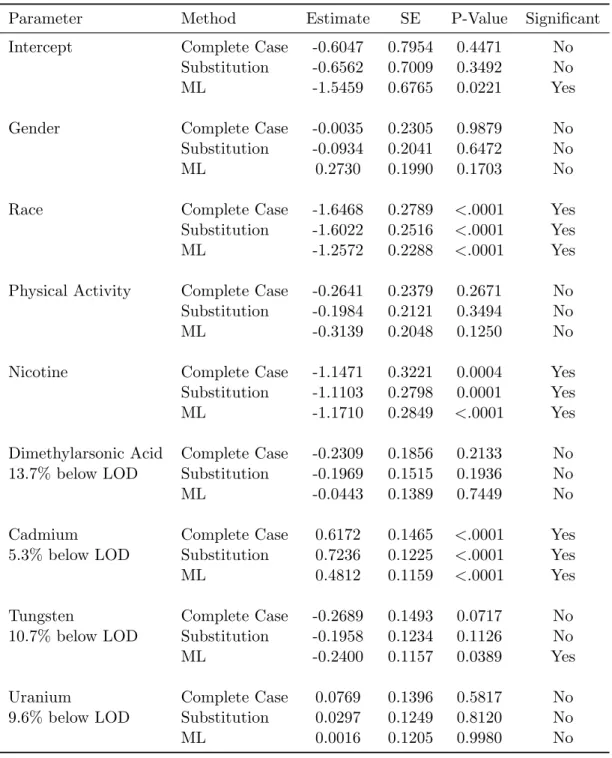
Table 2.2 summarizes the results of this study again comparing the maximum likelihood

approach to both a complete-case analysis and ad-hoc substitution of LOD/√2. The

substi-tution of LOD/√2 is particularly relevant in this case, as urinary heavy metals falling below

the limit of detection are actually reported by the NHANES researchers as LOD/√2 in the

available public data releases. As can be seen, the maximum likelihood approach results in significantly smaller standard errors for the parameter estimates when compared to

complete-case analysis, and slightly smaller than those obtained via substitution with LOD/√2. This

leads to a change in statistical significance (at theα= 0.05 level) for the effect of Tungsten on

(45)

table 2.1 were calculated as the standard error of the population of 1000 final beta estimates, one for each simulated dataset. These estimation procedures are not equivalent, and it is important to note this difference.

It should also be noted that the fitted model used here does not include age as a covariate in the prediction of cancer status. A logistic model including the age covariate was also fit to this data, and age was found to be highly significant. The current model (without an age covariate) has been included here to more clearly display the potential benefits of the proposed methodology.

2.6 Discussion

In this chapter, we have proposed a method of maximum-likelihood estimation in generalized linear models with an unlimited number of covariates subject to a limit of detection. We have proposed models for the joint covariate distribution, which is based on a sequence of one-dimensional conditional distributions. The methodology presented here can be easily extended to cases where both the response and the covariates are subject to a limit of detection. The maximum likelihood approach presented here is much simpler computationally than a direct computation by way of the observed-data likelihood, especially for cases with multiple covariates subject to a LOD. When only a single covariate (or just the response) is subject to a LOD, closed-form solutions can often be used.

For the example considered in Section 2.4, the variance estimates for β are significantly

improved over the complete case analysis. This result was echoed in our real-life analysis of NHANES data. This improvement can clearly lead to higher statistical power in studies that include data subject to detection limits.

(46)

Table 2.2: Logistic regression model summary for NHANES data, comparing maximum

like-lihood approach to complete case analysis and ad-hoc substitution of LOD/√2

Parameter Method Estimate SE P-Value Significant

Intercept Complete Case -0.6047 0.7954 0.4471 No

Substitution -0.6562 0.7009 0.3492 No

ML -1.5459 0.6765 0.0221 Yes

Gender Complete Case -0.0035 0.2305 0.9879 No

Substitution -0.0934 0.2041 0.6472 No

ML 0.2730 0.1990 0.1703 No

Race Complete Case -1.6468 0.2789 <.0001 Yes

Substitution -1.6022 0.2516 <.0001 Yes

ML -1.2572 0.2288 <.0001 Yes

Physical Activity Complete Case -0.2641 0.2379 0.2671 No

Substitution -0.1984 0.2121 0.3494 No

ML -0.3139 0.2048 0.1250 No

Nicotine Complete Case -1.1471 0.3221 0.0004 Yes

Substitution -1.1103 0.2798 0.0001 Yes

ML -1.1710 0.2849 <.0001 Yes

Dimethylarsonic Acid Complete Case -0.2309 0.1856 0.2133 No

13.7% below LOD Substitution -0.1969 0.1515 0.1936 No

ML -0.0443 0.1389 0.7449 No

Cadmium Complete Case 0.6172 0.1465 <.0001 Yes

5.3% below LOD Substitution 0.7236 0.1225 <.0001 Yes

ML 0.4812 0.1159 <.0001 Yes

Tungsten Complete Case -0.2689 0.1493 0.0717 No

10.7% below LOD Substitution -0.1958 0.1234 0.1126 No

ML -0.2400 0.1157 0.0389 Yes

Uranium Complete Case 0.0769 0.1396 0.5817 No

9.6% below LOD Substitution 0.0297 0.1249 0.8120 No

(47)

and straightforward. However, more complicated covariate distributions will require a less standard computation of the log-likelihood, which can take significant additional time and can lead to error.

For both the simulation study and real-data analysis presented here, mi = 250 samples

were taken for each observation with covariates below a limit of detection. Based on the authors experience and other extensive simulations performed with this type of data, we feel

that a sample size of at leastmi= 100 is necessary for accurate inference.

The computing time required to achieve EM convergence here clearly depends on the number of covariates in a model, the degree of censoring that is observed, and the number of samples that are taken for each censored observation. The simulation presented in Section 2.4 tended to converge quickly, with only an average of 28 iterations performed per dataset. This simulation of 1000 datasets took about 16 hours to complete on a Lenovo laptop with a dual-core Pentium processor, making this approach very computationally feasible.

(48)

Chapter 3 Joint Modeling of Longitudinal and

Survival Data with Missing and

Left-Censored Time-Varying Covariates

3.1 Introduction

In many longitudinal studies, time to event data is recorded in addition to the longitudinal and baseline covariates. In such studies, interest often lies in understanding the relationships between the longitudinal history of a process and it’s effect on the risk of an event. For analysis

of this type of data, a class of models called joint models has been developed, which jointly

(49)

is motivated by data from the Multicenter AIDS Cohort Study (MACS, Kaslow 1987), a prospective study of disease progression in participants infected with, or at risk for infection with, HIV. The subset of MACS participants who seroconvert with HIV while under obser-vation are followed from the date of HIV seroconversion, with many variables including CD4 cell counts and viral load measured at planned study visits every 6 months. Interest lies in the progression of CD4 cell counts and viral load from seroconversion with HIV, and their impact on survival. Of the available viral load data, 27% is missing and 17% falls below a limit of detection. Using a Bayesian analysis, we model the progression of CD4 cell counts over time, while accounting for the missingness and left-censoring on the available viral load data. We assume that the intermittent missingness is missing at random (MAR, Little 1995). Although a great deal of attention has been paid to developing joint models in recent years, the literature on censored and/or missing covariate data within a joint model is sparse. A paper by Wu et al. (2008) investigated the joint modeling in an AIDS clinical trial with informative dropout. This paper incorporated a missing data mechanism into the joint model likelihood, to model missingness in the model covariates due to subject dropout. Estimation was performed using an EM algorithm. To the authors knowledge, no paper has investigated joint modeling with intermittent missing covariate data, or with covariate data subject to a limit of detection. Using data from the Multicenter AIDS Cohort Study, the goal of the analysis presented in this chapter is to jointly model the longitudinal progression of disease in study participants while accounting for both intermittent missingness and a limit of detection on a single covariate. Estimation will be undertaken using a Bayesian framework, which contrasts with the EM approach taken in the Wu et al. (2008) paper.

Estimation Methods for Data Subject to Detection Limits