Dynamic real-time substrate feed optimization of anaerobic co-digestion plants

(1)

The handle

http://hdl.handle.net/1887/29085

holds various files of this Leiden University

dissertation

Author: Gaida, Daniel

(2)

Dynamic Real-Time Substrate Feed Optimization of

Anaerobic Co-Digestion Plants

Proefschrift

ter verkrijging van

de graad van Doctor aan de Universiteit Leiden, op gezag van Rector Magniﬁcus prof. mr. C.J.J.M. Stolker,

volgens besluit van het College voor Promoties te verdedigen op woensdag 22 oktober 2014

klokke 11:15 uur

door

Daniel Gaida

(3)

Promotor: Prof. Dr. T.H.W. Bäck

Prof. Dr. M. Bongards (Cologne University of Applied Sciences) Voorzitter: Prof. Dr. J.N. Kok

Overige leden: Prof. Dr. U. Jumar (University of Magdeburg) Prof. Dr. A. Plaat

Dr. M.T.M. Emmerich Dr. E.A. Schultes

(4)

(5)

(6)

Chapter 1 Introduction

The European Union (EU) has set a goal that 20 % of the gross ﬁnal energy consumption in the EU should be produced by renewable energy sources in the year 2020 (Holm-Nielsen et al., 2009). Between the years 2004 and 2011 in the EU this share increased from8.1% to13.0 % (Eurostat, 2013).

In Germany7.0% of the gross electrical energy production in 2012 was produced out of biomass (22.6% of gross electrical energy production was from renewable sources), whereas biogas produced from biomass had the greatest share (FNR, 2013). Biogas mainly consists of methane and carbon dioxide and is produced in so-called biogas plants. In such plants, one of the key components is the digester. In the digesters there is an absence of oxygen, allowing the bacteria to convert the anaerobic degradable biomass in to biogas. Some examples for biomass are manure, grass, energy crops, organic fraction of municipal solid waste (OFMSW), biodegradable wastes from industrial production, wastewater and many more.

Once produced, there are various utilization pathways for biogas. Among them are production of heat (e.g. in third world countries) as well as of electrical and thermal energy while burning it in cogeneration units (also called combined heat and power plants (CHP)) and upgrading biogas to biomethane by removal of carbon dioxide. The latter allowing for the possibilities of either injecting the biomethane into the natural gas grid or utilizing it as vehicle fuel (Holm-Nielsen et al., 2009).

(11)

valuable resources is absolutely necessary. This aspect is also considered in the recently announced new 2014 Renewable Energy Sources Act. The ﬁrst draft suggests that the German government is focusing on the digestion of waste products in the near future, thus trying to reduce ecological costs introduced by the cultivation of maize for energy production.1

The Netherlands was ranked at the 5th position regarding primary biogas production in the EU in the year 2011 (OBSERV’ER, 2012). In 2013, there was a total of105 co-digestion plants with an installed electrical power of129 MW (Agentschap NL, 2013). The current funding scheme for renewable energy in the Netherlands is the Renewable Energy Production Incentive Scheme (SDE+, Dutch: stimuleringsregeling duurzame energieproductie) (Statistics Netherlands, 2012). In 2012 the renewable energy share of gross ﬁnal energy consumption in the Netherlands was4.4% with the 2020 goal being 14% (Centraal Bureau voor de Statistiek, 2013).

Operation of biogas plants is only economically feasible if they are operated near their optimal operating point. One key aspect for optimization is to choose the most suitable biomasses, called substrates, and their daily throughput. The substrates used strongly effect biogas production, population sizes of different bacteria species in the digesters and digestate quality. Thus, by optimizing the substrate feed, economical, ecological and stability criteria of plant operation can be optimized. At present, most biogas plants in Germany are operated at steady-state, ideally producing sufficient biogas to power an electrical generator at maximum capacity. This allowed biogas plant owners to ensure that they obtained the maximum possible funding (BMU, 2009), until the EEG was amended in 2012. The 2012 amendment introduced the possibility for biogas plants to sell the produced electrical energy directly to an interested customer (BMU, 2012a). Consequently, higher revenues compared to conventional remuneration schemes are possible. Selling energy under the EEG feed-in tariff on EPEX SPOT’s Day-Ahead market became an interesting option. EPEX SPOT2_{is a European power spot market}

covering France, Germany, Austria and Switzerland. Therefore, there is a need for highly ﬂexible biogas and power production, which in turn requires a closed-loop substrate feed control that is able to track a given setpoint and adjust the substrate mix in an optimal manner.

The current state of control and automation on most full-scale biogas plants is very basic (Wiese and König, 2009). On agricultural biogas plants (ABP) the substrate feed is usually changed on a daily basis based on simple calculations or a rule of thumb (Dewil et al., 2011). Due to a lack of online process instrumentation, it is often not possible to make reliable predictions of expected biogas production and the state of the process. Advances in the development of reliable and robust measurement sensors, as

(12)

1.1. Aim and Objectives 7

well as detailed anaerobic digestion (AD) models give hope that these limitations will be lifted in the coming years (Madsen et al., 2011). Nevertheless, it is questionable as to whether biogas plants will ever have adequate instrumentation ﬁtted as standard. Therefore, presently and in the future, control and optimization methods ﬁtted to biogas plants should cope with these limitations. Following this idea in this thesis, the developed real-time feed optimization method requires only very basic instrumentation, so that it will be possible to use it on ordinary full-scale biogas plants.

However, simulation and control of waste digestion is much more challenging than for ABPs. The reason is that feed based on municipal waste will change its composition continuously, requiring continuous adjustment and control of the plant. Nevertheless, the dissemination of the technologies developed in this work will be absorbed by a market that speciﬁcally requires these solutions.

1.1 Aim and Objectives

In this thesis a dynamic real-time optimization (RTO) scheme is developed to achieve optimal substrate feed control for biogas plants. RTO continually alters the substrate feed to maximize the economic productivity of the biogas plant while at the same time predeﬁned stability criteria are maintained. In Figure 1.1 the developed dynamic RTO control loop is visualized. An important part of the dynamic RTO scheme is the

RTO

Σ process_control biogas_plant

state estimator optimal feed

Q∗ch4(t) ech4(t) feed

−

Qch4(t)

ˆ

xk

disturbances

y

Figure 1.1: Dynamic Real-Time Substrate Feed Optimization. The RTO determines the

optimal substrate feed and returns the optimal volumetric methane ﬂow rate Q∗_ch₄(t). The

process control adapts the optimal feed to stabilize the produced methane ﬂow rateQch4(t)of

the biogas plant around the given setpointQ∗_ch₄(t). As a dynamic model is used for prediction,

a state estimator is needed that estimates at each time stepk the current state estimatexkˆ

given the current feed and plant measurementsy.

(13)

The developed method for the dynamic real-time substrate feed optimization is dedicated to assisting the biogas plant operators in the selection of the optimal substrate feed on a daily basis, ultimately with the goal of autonomously controlling the feed of the plant. The following features are expected from the RTO scheme:

• Determination of optimal substrate mixture for anaerobic co-digestion plants. • Keeping the plant stable by all means due to prediction.

• Consideration of changing substrate availabilities in the chosen substrate feed. • Robust stable setpoint tracking.

• Flexibility and extensibility with respect to the optimization goal.

In order to realize a sophisticated real-time feed optimization that is practical to implement, there are multiple objectives that must be achieved.

The first objective is to create a detailed dynamic simulation model for biogas plants. This model is used in the dynamic RTO to continually predict the optimal substrate feed for the controlled plant. Performance and practical usability of RTO is highly dependent upon the underlying model, consequently, a significant amount of effort is necessary to ensure realistic modeling of full-scale biogas plants.

The optimization and prediction method implemented as a part of the RTO scheme, is nonlinear model predictive control (NMPC). Thus, the second objective is to develop and implement NMPC for the substrate feed of biogas plants. NMPC selects a substrate feed trajectory that optimizes an objective function over a prediction horizon. For biogas plants, such an objective function may contain economical, ecological and stability criteria and thus is of a multi-objective nature. Furthermore, it can be highly nonlinear. To solve the nonlinear multi-objective optimization problem, global multi-objective optimization methods such as evolutionary algorithms and eﬃcient global optimization (EGO) are used.

In order to make NMPC predictions with the simulation model, the NMPC must know the current system state of the biogas plant. Therefore, the third objective is to develop a state estimation algorithm that is capable to continually estimate the state of the biogas plant. The challenge to develop a reliable state estimator increases with process model complexity. To achieve this task, supervised machine learning methods are used to estimate the current state given current and past measurement data.

1.2 Main Contributions of this Thesis

To the author’s knowledge, dynamic real-time substrate feed optimization has not been applied to anaerobic co-digestion plants before. To achieve this goal, different components from various scientific fields had to be developed, implemented and combined. This is the first main contribution of this thesis.

(14)

1.3. Outline of this Thesis 9

at present. There are multiple challenges when attempting to implement this model inside the NMPC. Three of these challenges are that predictions are time consuming, the underlying optimization problem is highly nonlinear and the state estimator must estimate a large state vector of a non observable process. To address the ﬁrst two challenges, evolution strategies are used that in part use surrogate models to improve speed.

Solving the latter challenge results in the second main contribution of this thesis. This is the development of the state estimation algorithm. Using machine learning methods, a static function is created that maps measured process values to the state vector of the plant and therefore can be used for state estimation. Classical state estimation approaches such as the famous Kalman ﬁlter will not be stable because the observability criterion (Simon, 2006) in practice is not satisﬁed for the ADM1. Therefore, this new state estimation approach is needed.

The last contribution of this thesis to the scientiﬁc community is the MATLAB®

toolbox for “Simulation, Control & Optimization of Biogas Plants” (Appendix B), which was developed for the purposes of this thesis.

1.3 Outline of this Thesis

This document is structured in ﬁve parts.

Part I presents the theoretical foundation to this work. As the proposed real-time optimization scheme uses multi-objective model predictive control, Chapter 2 presents the basics of model predictive control and multi-objective model predictive control. To solve the multi-objective optimization problem formulated in Chapter 2, Chapter 3 reviews multi-objective optimization algorithms which will be used to solve the control problem. They are SMS-EMOA and SMS-EGO which are based on theS-Metric. For

model predictive control a state estimation algorithm is necessary. Therefore, three diﬀerent state estimation algorithms are described in Chapter 4 which concludes Part I. The state estimation algorithms are the well-known hybrid extended Kalman ﬁlter, moving horizon estimation and the newly developed state estimator based on machine learning methods. Using a simple model of an anaerobic digestion process, all three approaches are validated and compared.

(15)

The 3rd part, Part III, starts with Chapter 8 that presents the results obtained with the self-developed state estimator for the biogas plant model of Chapter 7. Chapter 9 outlines the main result of this thesis, the dynamic real-time substrate feed optimization for co-digestion plants. The proposed RTO scheme is validated by means of extensive simulation and optimization studies revealing its performance.

The thesis is concluded by Chapter 10, in which the main results of this thesis and possible future work are summarized.

In the appendices, detailed technical descriptions of the used models are provided. In Part A of the appendix the AD model used in the experiments of Chapter 4 is presented. Part B presents the MATLAB®_{toolbox developed for this thesis in which all}

(16)

Part I

(17)

(18)

Introduction

In this ﬁrst part of the thesis three of the four key ingredients of dynamic real-time optimization (RTO) are discussed in detail:

• Multi-Objective Nonlinear Model Predictive Control (MONMPC) (Chapter 2) • Multi-Objective Optimization Algorithm (Chapter 3)

• State Estimation Method (Chapter 4) • Dynamic Process Model (Chapter 7)

The fourth item, namely the dynamic process model, is not dealt with in this part, but in Chapter 7.

Indynamic real-time optimizationa dynamic simulation model is used to develop a predictive control. In general a RTO system is an upper-level control that provides a setpoint to a lower-level control (Engell, 2007). In the upper-level control the simulation model is used to predict the future economics of the controlled plant, whereas an optimization method generates the setpoint, so that future profits are maximized. The lower-level control holds the controlled variable around the given setpoint. Usually the setpoints are created on a medium time-scale (hours to days) whereas the lower-level control acts on a shorter time-scale such as seconds to minutes, cf. Darby et al. (2011). Multi-objective nonlinear model predictive controlis used in the RTO scheme to continually find optimal substrate feed trajectories over a prediction horizon. The objective function usually comprises terms to maximize the profit, minimize the ecological impact, and to maintain the plant stable at all times. Using the model of the process, different feed trajectories can be evaluated, whereas only the optimal trajectory is applied to the real biogas plant for a much shorter control sampling time. Excellent overviews about nonlinear model predictive control can e.g. be found in Morari and H. Lee (1999), Findeisen et al. (2003), Johansen (2011) and Mayne et al. (2000).

Multi-objective optimization algorithms are used to solve the optimization problem stated by the MONMPC. As the optimization problem is nonlinear, the focus is put on global optimization methods, such as multi-objective evolutionary algorithms (Fleming and Purshouse, 2002).

(19)

(20)

Chapter 2 Multi-Objective Nonlinear Model

Pre-dictive Control

Consider a physical, time-dependent, real-world system showing deterministic behavior at any timet∈_R+

0. Assume that the main inﬂuence on the system by its environment

can be described by a ﬁnite number nu ∈N0 of physical values. They are called the

input values of the system. The nominal input values of the system are generated by a function of time u : R+0 → U, which, for each time t ≥ 0, returns the input of

the system at time t symbolized by u(t) ∈ U. Each input function uiu, with u := (u1, . . . , uiu, . . . , unu)

T

, returns values out of the setUiu⊆R,iu= 1, . . . , nu. The setU then is deﬁned asU := (Uiu)

nu _:=_U

1× · · · × Unu. Note that the ith input of the system is symbolized by the iteratori_u∈ {1, . . . , n_u}.

Those physical values which are assumed to describe the inherent behavior of the system are put inside the state of the system x : R+0 → X, with the state space

X ⊆Rnx andnx ∈N0 representing the number of physical values in the system state

vectorx∈ X. The idea of the system state is that if it is known for some timet, then

the complete physical system description at that time is known. Examples of state vector components are the position of the system in space, the temperature inside the system or the concentration of ﬂuids or species inside the system.

The setsX andU could be generated out of state and input constraints, respectively.

If the state (input) constraints are linear, then X (U) is a convex set (Boyd and Vandenberghe, 2004).

To be able to predict the future trajectory of the system state x for a given input

trajectoryuthe real-world system is described as a system of continuous-time nonlinear

stochastic diﬀerential equations:

o_x0

(t) =f(ox(t),u(t),ω(t)), ox(0) =x(0). (2.1)

This future state vector trajectory is symbolized by the vector valued function o_x _:

(21)

called the open loop state, whereas “open” is symbolized by theo in front of _xino_x.

The behavior of the real-world system is approximately modeled using the real-valued smooth vector ﬁeldf :X ×U ×_Rnω→ T X, which maps the input space of the function

onto the tangent spaceT X ⊆Rnx. To emphasize that f is only an approximation of

the real system the noise processω:_R+₀ →Rnω is introduced as input of the system

functionf. This noise process is used to take account for the fact thatfcannot describe

exactly what is happening in the real world and for possibly noisy input values u.

This nω ∈ N0 dimensional noise process ω is modeled as a normal distribution with

zero-mean and the covariance matrixΨω∈Rnω×nω, symbolized by_ω₍_t₎_{∼ N}₍₀_,_Ψ

ω). We assume stationary, white noise. That is,E

ω(t)·ωT₍_τ₎

=Ψω·δD(t−τ), where

δ_D is the Dirac delta “function” andEh·idenotes the expected value.

Given the initial state of the real system at time t = 0, x(0), for each t ≥ 0 the approximate state of the systemo_x₍_t₎ can be calculated using equation (2.1). As for

t > 0 there is no further interaction with the real system (thus no feedback) this predictor could be very inaccurate, because it cannot be guaranteed that the predicted state valueso_x₍_t₎track the real state values _x₍_t₎for_{t >}₀. The error between the two

state vector trajectories is commonly measured by the root-mean-square error (RMSE): RMSE(ox(t),x(t)) :=

(

o_x₍_t₎

−x(t))·(ox(t)−x(t))T ₂,

whose value must be kept arbitrarily small. Better predictors than eq. (2.1) are presented later in Chapter 4.

The task at hand is to ﬁnd an optimal input function u∗ : R+0 → U, such that an

objective function

e

J :X × U →_Rno (2.2)

gets minimized for all t ∈ [0,∞), with the number of objectives n_o ∈ N0 and the

constraint o_x₍_t₎ _{∈ X ∀}_t _∈ _[0_,_∞₎. The vector function

e

J := Je1, . . . ,Jeno T

consists out ofn_o scalar-valued objective functions

e

Jio :X × U →R (2.3)

withi_o= 1, . . . , n_o. The problem can be formulated as:

minimizeu Je(ox(t),u(t)) subject to o_x0

(t) =f(ox(t),u(t),0), ox(0) =x(0),

o_x₍_t₎_{∈ X}_, _∀_t_≥₀_,

u: [0,∞)→ U.

(2.4)

(22)

2.1. Case I: Number of Objectivesn_o= 1 17

functionJeio separately is often not well-suited, because most of the time the objective functions are conflicting. Two objective functions are conflicting, if and only if the set of optimal solutions of one objective function does not overlap with the set of optimal solutions of the other objective function. To simplify things, at first the optimal control problem for the casen_o= 1is handled in Section 2.1 before the general case forn_o>1 is solved in Section 2.3. To minimize the objective functionJeproperly, concepts from multi-objective optimization are used, which are recapped in Section 2.2.

Since minimizing Jein choosing the optimal input u for all t ∈[0,∞) is in general a hard problem, in practice a heuristic technique named multi-objective nonlinear model predictive control (MONMPC) shall be used that will be introduced in Section 2.1.

2.1 Case I: Number of Objectives

n

_o

= 1

For n_o = 1 the objective function reduces to the scalar-valued objective functionJe1,

deﬁned in equation (2.3), such that the minimum of the objective function is well deﬁned. Thus, for this case problem (2.4) results in the problem formulation:

u∗:=arg min u Je1(

o_x₍_t₎_,_u₍_t₎₎

subject to o_x0₍_t_{) =}_f₍o_x₍_t₎_,_u₍_t₎_,₀₎_, o_x_{(0) =}_x₍₀₎_, o_x₍_t₎_{∈ X}_, _∀_t_≥₀_,

u: [0,∞)→ U.

(2.5)

Problem (2.5) states that we try to ﬁnd the optimal input functionu∗for system (2.1)

which for all timet≥0minimizes the objective functionJe1.

According to Diehl et al. (2006a) there are three basic approaches to address optimal control problems:

• Dynamic Programming Methods • Indirect Methods

• Direct Methods

Direct methods can be divided into single shooting, collocation and multiple shooting. The approach followed in this thesis belongs to the method of single shooting. An example of multiple shooting can be found in Diehl et al. (2002, 2003). For collocation see Biegler (1984).

Finding a closed solution for this problem using dynamic programming or indirect methods can be very diﬃcult or even impossible for some systems f and objective

functionsJe1(Findeisen et al., 2003, Diehl et al., 2006a). From a practical viewpoint a

closed solution is often not needed, because model mismatch and disturbances acting on the real-world system (both modeled by the noise processω) will make the solution

(23)

Therefore, using nonlinear model predictive control (NMPC), problem (2.5) is only solved over a ﬁnite horizon. This ﬁnite horizon is called the prediction horizonTp∈R+.

Having solved problem (2.5) over the prediction horizonT_p>0, the optimal input is applied to the system for a short time period, named (control) sampling timeδ. After

the sampling time δ∈ R+ has passed by, problem (2.5) is solved over the prediction

horizon again. ThereforeTpis moved forward by timeδand the new solution is applied

again for timespanδ and so on. Therefore, problem (2.5) is solved iteratively over the

moving horizonT_p, resulting in an approximate solution to problem (2.5).

For Tp → ∞ and δ → 0 the found approximate solution will converge towards the optimal solutionu∗, provided it exists.

The found optimal input functions at each iteration cannot be equal to the input values applied to the system, because they are only deﬁned over the time periodTp. Thus, the

found optimal inputs are called open loop input functions. The applied input function to the system is named closed-loop input.

The NMPC approach has at least two justiﬁcations:

• As there may be no closed solution to problem (2.5), the approach using NMPC will at least return an approximate solution. The degree of approximation can be deﬁned by the user in choosing appropriate values for the prediction horizonT_p

and sampling timeδ.

• Because of model mismatch and disturbances a solution has to be calculated repeatedly, anyway. Therefore, there is no need to spend time in solving problem (2.5) over an inﬁnite horizon.

Next to prediction horizonT_pand sampling timeδ, the term control horizonT_c∈_R+

with Tp ≥ Tc ≥ δ is used as well. Using these terms it can be stated that for each

sampling instancek= 0,1,2, . . . at time

tk :=k·δ (2.6)

NMPC tries to ﬁnd the optimal open loop input function o_u∗

k : [tk, tk+Tp] → U

which minimizes the objective functionJe1over the interval[tk, tk+Tp], deﬁned by the

prediction horizonT_p. Open loop input functions are denoted byo_u_{: [}_t

k, tk+Tp]→ U.

During the time period[tk, tk+Tc] the system input ou may be changed, after that

it is kept constant at the valueo_u₍_t

(24)

2.1. Case I: Number of Objectivesn_o= 1 19

(2.5) can be formulated approximately as:

For eachk= 0,1,2, . . . settk =k·δand solve:

o_u∗

k:=arg mino_u Je1(

o_x₍_τ₎_,o_u₍_τ₎₎

subject to o_x0

(τ) =f(ox(τ),ou(τ),0), ox(tk) =x(tk),

o_x₍_τ₎_{∈ X}_, _∀_τ_∈_[_t

k, tk+Tp], o_u_{: [}_t

k, tk+Tc]→ U, o_u₍_τ_{) =}o_u₍_t

k+Tc), ∀τ∈(tk+Tc, tk+Tp].

(2.7)

Here it is assumed that for each discrete timetkthe statex(tk)of the real system can

be observed. As the system state often can not be observed directly, it often has to be estimated for each timetk, see Chapter 4.

The resulting optimal inputo_u∗

k is applied for the interval [tk, tk+δ)to the system:

u(t) =ou∗_k(t), t∈[tk, tk+δ) (2.8)

and the optimization problem in (2.7) is solved again for the next value ofk. Note that

we assume here that problem (2.7) can be solved in no time. If we would take into account, that a method solving problem (2.7) for onekneeds a certain runtime, then

the application of the optimal input to the real system according to equation (2.8) will be delayed by the timespan of the runtime.

To simplify the NMPC problem (2.7) further, the open loop inputo_uis often restricted

to be a piecewise constant function. Therefore, given the open loop input function

o_u _{:= (}o_u

1, . . . ,ouiu, . . . ,ounu)

T_{, each component} o_u

iu : R+ → Uiu is a piecewise constant function. The duration of each constant period of the function o_u

iu is given by the sampling timeδ. In problem (2.7) it is deﬁned that the open loop inputoushould

only be variable over the control horizonT_c. Then, the number of steps of the piecewise

constant function over the control horizon Tc is given bysc := T_δc ∈ N0. Thus, each

such piecewise constant functiono_u

iu of theiu= 1, . . . , nuinputs can be described by sc values given in the vectoruiu:= (uiu,1, . . . , uiu,sc)

T

∈(Uiu)

sc _{with the}_i_{= 1}_{, . . . , s}

c

amplitudesuiu,i∈ Uiu as given in equation (2.9). This kind of parametrization is called control vector parametrization (Schlegel et al., 2005). An example of such a piecewise constant input function is depicted in Figure 2.1.

o_u

iu(tk+τ) :=

 



sc P

i=1

uiu,i·rect(τ−(i−1)·δ) 0≤τ < Tc

uiu,sc Tc ≤τ ≤Tp

rect(τ) := (

1 0≤τ < δ

0 else

(25)

Furthermore, we deﬁne

u:= uT1, . . . ,uTiu, . . . ,u

T nu

T

∈ UF,with

UF := (U1)

sc_{× · · · ×}₍_U

iu)

sc_{× · · · ×}₍_U

nu)

sc_, (2.10)

containing all s_c amplitudes of each of the n_u inputs, which therefore completely

describes the piecewise constant open loop input functiono_u. Using this simpliﬁcation

0 δ 2δ 3δ Tc Tp τ

o_u 1(τ)

u1,1

u1,2

u1,3

u1,4

Figure 2.1: Example of a piecewise constant open loop input function o_u

1 for iu = 1 and

number of stepssc= 4.

the problem in ﬁnding a continuous function o_u over the interval _[_t

k, tk+Tc] was

transformed into the simpler problem of ﬁnding a vector u containing only n_v :=

sc·nu ∈ N0 components, i.e., the amplitudes of the piecewise constant inputs. This

means, that the argument of the objective functionJeis changed from a function ou to a vector u with nu elements. From now on this vector u is called the vector of

optimization or decision variables, containingn_uoptimization variables.

The transformation between the vector of optimization variablesuand the open loop

input functiono_uis given by the function

fU:UF→ U (2.11)

which returns the piecewise constant function

o_u_{: [}_t

k, tk+Tp]7→fU(u) (2.12) given the corresponding vector of optimization variablesu using equation (2.9).

To account for this transformation in optimization problem (2.7) a new objective function with a diﬀerent domain J : X × UF → Rno has to be introduced. Using

equation (2.11) the objective functionJ is deﬁned by the following equation:

e

J(ox(τ),ou(τ))(2.11)= Je(ox(τ),fU(u)) =:J(ox(τ),u) ∀τ∈[tk, tk+Tp] (2.13)

Using the new objective function J := (J1, . . . , Jno)

T_{, with}

Jio : X × UF → R and

introducingu∗_k ∈ UF, with

o_u∗

(26)

2.2. Multi-Objective Optimization 21

problem (2.7) can be reformulated as:

For each k= 0,1,2, . . . set tk=k·δand solve:

u∗_k :=arg min u∈UF

J1(ox(τ),u)

subject to o_x0

o_x₍_τ₎_{∈ X}_, _∀_τ _∈_[_t

k, tk+Tp], o_u_{: [}_t

k, tk+Tp]→fU(u).

(2.15)

Aso_u∗

k (2.14)

= fU(u∗k), equation (2.8) can be applied.

To stress that the open loop input u is the vector of optimization variables, which

therefore is the only grip to inﬂuence the values of the objective function, if necessary the following notation is used:

Jx(u) :=J(ox(τ),u). (2.16) The functionJx:UF →Rno, Jx:= (Jx,1, . . . , Jx,no)

T_{, will be used in Section 2.2 to}

simplify the notation,Jx,io :UF →Rforio= 1, . . . , n_o.

2.2 Multi-Objective Optimization

To be able to solve problem (2.4) for n_o > 1 the concept of multi-objective optim-ization is introduced. In multi-objective optimoptim-ization one tries to solve the following optimization problem:

minimizeu Jx(u) subject to u∈ UF

(2.17)

To solve (2.17) a couple of terms are deﬁned to get an idea of how to minimize the vector functionJx.

In Deﬁnition 2.1 the notationJx(u1)≤Jx(u2)is used, which is short forJx,io(u1)≤

Jx,io(u2)∀io∈ {1, . . . , no}, foru1,u2∈ UF.

Deﬁnition 2.1 (Custódio et al. (2012)):Given two vectors of optimization variables

u1,u2 ∈ UF, it is said that u1 dominates u2, being represented by u1 ≺ u2, iﬀ

Jx(u1)≤Jx(u2)andJx,io(u1)< Jx,io(u2)∃io∈ {1, . . . , no}.

As Jx shall be minimized, u1 is always preferred over u2, if u1 ≺u2. Deﬁnition 2.1

implies that u1 ≺u2 if and only if Jx(u1)≤Jx(u2) and Jx(u1)6= Jx(u2). Some

authors deﬁne the dominance relation in the space of objective function vectors. In this meaning there exists the following equivalence, which is used in this thesis:

(27)

Special interest lies in vectors of optimization variables u which are non-dominated

within a given set. They are called Pareto optimal points, see Deﬁnition 2.2.

Deﬁnition 2.2(Coello Coello (2011)):It is said that a vector of optimization variables

u∗∈ UF isPareto optimaliﬀ there does not exist anotheru∈ UF such thatu≺u∗. Pareto optimal points are so-called trade-oﬀ solutions. There is no solution which is better (viz. smaller) in all components, but there could be solutions which are at least better in some component(s) and in each case worse in other components.

If, foru1,u2∈ UF,u1⊀u2andu2⊀u1thenu1andu2are said to be nondominated

points. A subset of UF is said to be nondominated when any pair of points in this subset is nondominated (Custódio et al., 2012).

Deﬁnition 2.3(Coello Coello (2011)):ThePareto optimal set P∗ is deﬁned by:

P∗:={u∈ UF|uis Pareto optimal}

Out of deﬁnition the Pareto optimal set is a nondominated set. The Pareto optimal set contains all Pareto optimal points in the feasible setUF. As for each vector in the Pareto optimal set, there does not exist a better (in the sense of domination) solution candidate with respect to problem (2.17), each Pareto optimal point will minimize the objective functionJx. In other words, all Pareto optimal points are equally good, thus

there is no ranking of Pareto optimal points at the moment. This is why we want to know the Pareto optimal set for the given problem (2.17). A set which contains only a subset of all Pareto optimal points is called approximate Pareto set or just Pareto set. As will be shown later in Chapter 3, it usually is not possible to ﬁnd the Pareto optimal set but only an approximate Pareto set, because only a ﬁnite number of Pareto optimal points can be found.

To the Pareto optimal set there does also exist the corresponding Pareto front, see Figure 2.2, deﬁned as:

Deﬁnition 2.4(Coello Coello (2011)):ThePareto front PF∗ is deﬁned by: PF∗:={Jx(u)∈Rno|u∈ P∗}

To each approximate Pareto set there does also exist an approximate Pareto front. So later the question will be to ﬁnd the best ﬁnite set of solutions, which approximates the Pareto front best possibly.

(28)

2.4. Case II: Number of Objectivesn_o>1 23

Jx,1

Jx,2 PF∗

º º

º

feasible points

infeasible point

Pareto optimal points •

•

• •

•

Figure 2.2:Example of a two-dimensional Pareto front. The Pareto front is depicted as a line.

Feasible points lie on the right side of the line, infeasible points on the left side. Pareto optimal points are feasible points which lie directly on the Pareto front.

2.3 Case II: Number of Objectives

n

_o

>

1

Knowing that the minima of the objective functionJ lie on the Pareto front, problem

(2.4) is approximately solved by:

For each k= 0,1,2, . . . set tk=k·δand solve:

PF∗_k:= min u∈UF

J(ox(τ),u)

subject to o_x0

o_x₍_τ₎_{∈ X}_, _∀_τ _∈_[_t

k, tk+Tp], o_u_{: [}_t

k, tk+Tp]→fU(u).

(2.18)

Let P∗

k be the corresponding Pareto optimal set to the Pareto front PF

∗

k for each

k= 0,1,2, . . .. Then the optimal input u∗_k ∈ UF has to be picked out of the solutions inside the Pareto optimal setP∗

k. One possible approach would be the use of a weighted

sum:

u∗k:=arg min

u∈P∗

k

no X

io=1

$io·Jx,io(u) (2.19)

with$io ∈(0,1),io= 1, . . . , noand

no P

io=1

$io = 1. The weights$io could also be made

dependent on the current state of the systemx(tk).

Other possibilities to determine the optimal inputu∗_kout of the Pareto optimal setP∗

k

(29)

2.4 Summary and Discussion

In this chapter an optimization problem was deﬁned, which states that an objective functionJeshall be minimized which depends on state trajectories of a dynamic system

o_x₍_t₎ and inputs _u₍_t₎, eq. (2.4). It was proposed to approximately solve this optimal

control problem using multi-objective nonlinear model predictive control. Applying NMPC resulted in the problem formulation (2.18):

For eachk= 0,1,2, . . . settk =k·δand solve:

PF∗_k := min u∈UF

J(ox(τ),u)

subject to o

x0(τ) =f(ox(τ),ou(τ),0), ox(tk) =x(tk), o

x(τ)∈ X, ∀τ∈[tk, tk+Tp],

o

u: [tk, tk+Tp]→fU(u).

(2.20)

with the optimal input vectoru∗_k in equation (2.19)

u∗_k :=arg min u∈P∗

k

no X

io=1

$io·Jx,io(u) (2.21)

and application of equation (2.8) which gives the optimal input in the interval t ∈

[tk, tk+δ)

u(t) =ou∗_k(t) =fU(u∗k), t∈[tk, tk+δ). (2.22)

As open questions remained how to solve the optimization problem in eq. (2.20) and how to get the state of the system at timetk,x(tk), in case it is not directly observable.

The ﬁrst question will be tackled in the next Chapter 3 and the latter question will be answered in Chapter 4.

(30)

Chapter 3 Multi-Objective Optimization

Algorithms

Multi-objective optimization algorithms try to find the Pareto front and the corres-ponding Pareto optimal set of a multi-objective optimization problem. As in case of continuous function optimization a Pareto front could contain infinite many elements these algorithms in general cannot find the complete Pareto front. Therefore they try to find solutions which approximate the form of the Pareto front best possible. In this thesis a multi-objective optimization algorithm is used to solve the MONMPC problem stated in Chapter 2. In the simulation and optimization studies in Chapter 9 two multi-objective optimization methods are compared. They are SMS-EMOA (Emmerich et al., 2005, Beume et al., 2007) and SMS-EGO (Wagner et al., 2007, Ponweiser et al., 2008). Both methods are briefly introduced in the following two sections.

Next to the two methods there are also other famous multi-objective optimization methods. Examples are NSGA-II (Deb et al., 2002), SPEA2 (Zitzler et al., 2001),

-MOEA (Deb et al., 2003) and ParEGO (Knowles, 2006). Various publications

comparing these diﬀerent multi-objective optimization methods reveal that both SMS-EMOA and SMS-EGO belong to the best methods of their kind, e.g. (Ponweiser et al., 2008, Wagner et al., 2007, 2010).

3.1 Hypervolume-based Evolutionary Algorithm

(31)

individual is measured by the objective function. In each iteration the population may change, what means that new solutions are created and already existing solutions are discarded from the population to keep the number of individuals inside the population constant. As EAs typically return a set of solutions (the population) in one call, they are especially suited to solve multi-objective optimization problems, compared to methods, which only return one solution at a time.

The purpose of a hypervolume-based EA is to maximize a scalar criterion, which is named the hypervolume indicator (or S-metric, Zitzler and Thiele (1998)), see

Deﬁnition 3.1. This criterion is a property of a set and describes the size of a space covered by this set. Below it is shown that the hypervolume indicator of the Pareto frontPF∗is maximal for a given optimization problem. Therefore, by maximizing the

hypervolume indicator the algorithm tries to ﬁnd the best approximation (with a ﬁnite number of elements) of the true Pareto frontPF∗. Note that the multi objectives are

mapped onto one objective, so that in general each single objective optimization method can be used to solve a multi-objective optimization problem using the hypervolume indicator (Fleischer, 2003, Knowles et al., 2003).

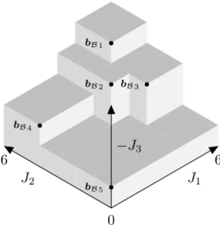
Deﬁnition 3.1 (Hypervolume indicator, Custódio et al. (2012)):The hypervolume indicator for some setA ⊂Rno and a reference pointr∈Rno that is dominated by all

the points inAis deﬁned as:

I_H(A) :=V ol{bB∈Rno|bB≤r∧ ∃aA∈ A:aA≤bB}=V ol [

aA∈A [aA,r]

!

HereV oldenotes the Lebesgue measure of ano-dimensional set of points, and[aA,r] denotes the interval box with lower corneraAand upper cornerr.

Figure 3.1a shows an example of the hypervolume indicator for a set A in a

two-dimensional and Figure 3.1b in a three-two-dimensional space. To be able to find the approximation of the Pareto front we first have to be able to compare two different approximate Pareto fronts and to decide which one is better.

Deﬁnition 3.2(Custódio et al. (2012)):Given two nondominated setsAandB.Ais

better thanB, which is represented byA ≺ B, if and only if

∀bB∈ B:∃aA∈ A:aA≤bB and∃bB∈ B:∃aA∈ A:aA≺bB

Now the hypervolume indicator is used to compare two Pareto front approximations. In Zitzler et al. (2003) it was shown, that if a certain property holds, the better nondominated set has a higher hypervolume indicator, see Lemma 3.1.

Lemma 3.1 (Custódio et al. (2012), Zitzler et al. (2003)):Let A and B be two

(32)

3.1. Hypervolume-based Evolutionary Algorithm 27

J1

J2

aA1

aA2

aA3

aA4

r

IH({aA1,aA2,aA3,aA4})

(a)The hypervolume indicator IH for the

setAis shaded in grey, cf. Custódio et al.

(2012).

bB2 bB3

bB4

bB1

bB5

6

0 6

J1

J2

−J3

(b) The hypervolume indicator IH for the

setB withr= (6,6,0)T, cf. Custódio et al.

(2012).

Figure 3.1: Hypervolume indicator for a set A := {aA1,aA2,aA3,aA4} ⊂ R2 in a

two-dimensional space and a setB:={bB1, . . . ,bB5} ⊂R3 in a three-dimensional space.

is the reference point used in the hypervolume computations. ThenIH(A)> IH(B).

This means that the hypervolume indicator of the true Pareto front is maximal, because it is always better than or equal to any other possible nondominated set, and therefore I_H(PF∗) ≥ I_H(A) for any nondominated set A. Knowing that, it is

obviously of interest to maximize the hypervolume indicator, so that the best possible approximation of the Pareto front can be found.

Furthermore in Zitzler et al. (2003) the following Lemma was shown.

Lemma 3.2 (Custódio et al. (2012), Zitzler et al. (2003)):Let ≺ be deﬁned as in

Deﬁnition 3.2, andA and B be two nondominated sets with the property ∀ϕ ∈ A ∪ B : ϕ ≺r, where r is the reference point used in the hypervolume computations. If

I_H(A)> I_H(B)thenB⊀A.

This means, that if an algorithm exists, which provably never decreases the hy-pervolume indicator of the current approximation of the Pareto front, then the approximation will never be worse than the approximation of the previous iteration. The S metric selection evolutionary multi-objective optimization algorithm

(33)

3.1.1 SMS-EMOA

SMS-EMOA is initialized with an initial populationP0 of size µ. In each iteration of

the algorithm one solution candidate ϕ is created out of the current population Pκ

using variation. If the new solution improves the quality of the current population it is kept and another solution is deleted, else it is discarded. The SMS-EMOA algorithm is shown in Algorithm 3.1.

Algorithm 3.1A SMS-EMOA algorithm (Beume et al., 2008) Input: P0←init

Input: κ←0 1:

2: repeat

3: ϕ←variation(Pκ)

4: D ←dominated_individuals(Pκ∪ {ϕ})

5: ifD 6=∅then

6: φ∗←arg maxφ∈Ddn(φ,Pκ∪ {ϕ})

7: else

8: φ∗←arg minφ∈(Pκ∪{ϕ})∆IH(Jx(φ),PFκ∪ {Jx(ϕ)})

9: end if

10: Pκ+1←(Pκ∪ {ϕ})\ {φ∗}

11: κ←κ+ 1

12: untilsome stopping criterion

In Algorithm 3.1 the number of dominating pointsdn(card(A)calculates the cardin-ality of the setA)

d_n(φ,A) :=card({aA∈ A |aA≺φ}) (3.1)

and the contributing hypervolume∆IH

∆IH(aA,A) :=IH(A)−IH(A\ {aA}) withaA∈ A

(3.2)

are used, cf. (Beume et al., 2007). In Algorithm 3.1 all dominated solutions are collected in the setDwhich are returned by the function dominated_individuals, called in line 4

of the algorithm. The population of solution candidates in iterationκis symbolized by

Pκ, which is the current approximation of the Pareto optimal set. The corresponding

approximation of the Pareto front is given byPFκ.

In Figure 3.2a the concept of the number of dominating pointsd_nis visualized. If there

are dominated solutions, visualized as the two white circles in Figure 3.2a, then d_n

(34)

3.2. SMS-EGO 29

J1

J2

φ∗

(a) The two dominated solutions (white circles) are dominated by solutions which lie in the shaded areas. The pointφ∗_{has the}

higher dominance number, which is three compared to one.

J1

J2

r

φ∗

(b)The dark shaded areas visualize∆IHof

the points, whereas the area of φ∗ is the

smallest.

Figure 3.2: The solutions of a two-dimensional optimization problem are shown. The worst

solutionφ∗will be deleted from the current population, cf. Beume et al. (2008).

then the solution with the smallest contributing hypervolume∆IHis deleted, see Figure

3.2b. As by discarding the solution with the smallest contribution always a subset of size µ with largest hypervolume is selected, the hypervolume indicator IH will never

decrease. Either the new solution is directly deleted from the population, which leaves the hypervolume indicator unchanged or the new solution increases the hypervolume indicator.

3.2 SMS-EGO

S-metric selection-based eﬃcient global optimization (SMS-EGO) was ﬁrst introduced

in Ponweiser et al. (2008). SMS-EGO is a multi-objective variant of so called Eﬃcient Global Optimization Algorithms (EGO) (Jones et al., 1998), which were earlier known as Statistical Global Optimization (Cox and John, 1997, Mockus et al., 1978). In SMS-EGO a meta-model is used to predict objective function evaluations, that are assumed to be expensive. The meta-model is learned from previous exact evaluations. Based on the meta-model it is decided which point is evaluated next using the exact objective function.

The general idea of SMS-EGO is to replace during optimization the original objective functionJwith the meta-model generated oneJb. Thus, an optimization method solves the optimization problem given by Jb. The returned optimal solution is evaluated by the original objective function J and this result is used to update the meta-model

(35)

For each componentJio of the objective function a separate meta-model is created. As meta-model a DACE stochastic process model is used, where DACE is short for ’Design and Analysis of Computer Experiments’ (Jones et al., 1998). Each such DACE model returns an estimate of the objective function_Jˆ_i

o∈Rand a standard deviationˆsJio ∈R representing the uncertainty in the estimation. Both values are collected in the vectors

b

J :=Jˆ1, . . . ,Jˆio, . . . ,Jˆno T

∈Rno andsˆJ := ˆsJ1, . . . ,sˆJio, . . . ,sˆJno T

∈Rno.

As the meta-models also return the estimated uncertainty sˆJ the lower conﬁdence boundJbpot:=Jb−αLCB·sˆJ, withαLCB=−Φ−_CDF1 0.5· no

√

0.5(Wagner et al., 2010, Emmerich et al., 2006), is used as the objective of some evaluated solution and not just

b

J. Here,Φ_CDF:R→(0,1) is the cumulative normal distribution function.

Each evaluatedJbis validated by a measure named additive -dominance, deﬁned in Def. 3.3.

Deﬁnition 3.3 (cf. Zitzler et al. (2003)):Given two vectors of optimization variables

u1,u2∈ UF, it is said thatu1-dominatesu2, being represented byu1+u2, iﬀ for

some∈R+ ∀io∈ {1, . . . , n_o}:Jx,io(u1)≤Jx,io(u2) +.

The single-objective function, which tries to ﬁnd the optimum of Jb uses additive

-dominance. It distinguishes between two kinds of solution candidates: -dominated

and non--dominated solution candidates, see Figure 3.3. Non--dominated candidates

ϕ_pot yielding Jbpot are evaluated based on the negative value of their additional hy-pervolume contribution:IH(PFκ)−IH

PFκ∪

n b

Jpot

o

, whereasPFκ is the current

approximation of the Pareto front ofJ. However, -dominated solutions are penalized

by a penalty given in equation (3.3), withPκ being the current approximation of the

Pareto optimal set (only containing non-dominated points), (Wagner et al., 2010).

p:=

      

maxϕ∈Pκ

"

−1 +

no Q

io=1

1 +maxJbpot,io−Jx,io(ϕ),0

#

ifϕ+ϕpot

0 otherwise

(3.3)

In equation (3.4) the single-objective function is shown, that is used to ﬁnd an optimal solution candidate to be evaluated at the original objective functionJ.

f_EGO:=  



IH(PFκ)−IH

PFκ∪

n b

Jpot

o

non--dominatedJbpot

p -dominatedJbpot

(3.4)

In SMS-EGO this objective function is minimized using an interior point method. The value for is calculated as in Ponweiser et al. (2008) using = ∆PFκ

(36)

3.2. SMS-EGO 31

There,∆PFκ:=max(PFκ)−min(PFκ), where

max(PFκ) :=

max Jx∈PFκ

Jx,1, . . . , max

Jx∈PFκ

Jx,io, . . . , max Jx∈PFκ

Jx,no T

,

likewise min(PFκ). Furthermore, c = 1− ₂1no is a correction factor and nleft is the number of remaining evaluations (Ponweiser et al., 2008).

J1

J2

r

penalty dominated

solution non--dominated

solution -dominated solution

additional hypervolume

Figure 3.3: Graphical explanation of the concept of -dominance used in SMS-EGO, cf.

(37)

(38)

Chapter 4 State Estimation

Given a real-world system as introduced in the beginning of Chapter 2 it can not be assumed that the state x of the system is known at each time t. Nevertheless,

the NMPC approach in eq. (2.20) assumes, thatxis known at each discrete timetk,

fork = 0,1,2, . . . (for the deﬁnition of tk see equation (2.6)). Those ny ∈N0 process

values that can be observed of a system are denoted by the measurement value function

y:_R+_{→ Y},_{Y ⊆}

Rny, and the functional connection of the current measurement values

y(t)and the current state of the systemx(t)is given by:

y(t) =h(x(t),υ(t)). (4.1)

Inaccuracies in the real-valued measurement function h : X ×Rnυ _{→ Y} as well as

measurement noise, are modeled by the nυ ∈ N0 dimensional white Gaussian noise

processυ:_R+_→

Rnυ with covariance matrix_Ψ

υ∈Rnυ×nυ.

The question arises, whether it is possible to estimate the values of the system state

x at each timetk, given equations (2.1) and (4.1) as well as u(τ) and y(τ) for each

τ ∈ [0, tk]. The state vector estimate at time tk will be symbolized using xˆ(tk) and

the corresponding function isxˆ :R+→ X. This state estimatexˆ will be used by the

NMPC (eq. (2.20)) as an approximation of the real statexat each timetk.

Let us assume that there are two diﬀerent sampling times where the measurement y

and input valuesuare acquired. The one for the measurement values is namedδy∈R+

and the one for the input valuesδ_u∈_R+. The ratio of the control sampling time_δ(see

Section 2.1) and both sampling timesδy ≤δand δu≤δ are deﬁned by the symbols:

Nδy := δ

δy ∈N0 and Nδu:=

δ

δu ∈N0. (4.2)

(39)

4.1 State Estimation using Software Sensors

In this section an approach is developed, that tries to ﬁnd a functionF_E:YNδy·k+1_×

UNδu·k+1_{→ X} with the sets

YNδy·k+1_:=_{y₍₀₎_,_y₍_δ_y₎_{, . . . ,}_y₍_δ₎_,_y₍_δ₊_δ_y₎_{, . . . ,}_y₍_t_k₎_} (4.3)

and

UNδu·k+1_:=_{u₍₀₎_,_u₍_δ

u), . . . ,u(δ),u(δ+δ_u), . . . ,u(tk)} (4.4)

estimating the state of the system at time tk. This function FE uses the complete

stream of inputs u and outputs y of the system recorded from time 0 until time tk

and therefore is a completely data based state estimator. Its returned state estimate ˆ

xFE :R+→ X deﬁned as

ˆ

xFE(tk) :=FE



  

y(0), . . . ,y(tk)

| {z }

∈ YNδy·k+1

,u(0), . . . ,u(tk)

| {z }

∈ UNδu·k+1 

  

∈ X (4.5)

would be the best state estimate that could be achieved based on the input and output data. Unfortunately the amount of data used in this approach is increasing with timetk,

therefore in practice it will only be possible to ﬁnd an approximation of this function

F_E, deﬁned as F˜_E : YNy+1_{× U}Nu+1 _{→ X}. There a constant number of input and

output samples is used, which areNu+ 1∈Nand Ny+ 1∈Nusing a sliding window

approach. To be able to interpret N_y and N_u some formalism has to be introduced.

To make the domain of_F˜_E_{sufficiently small, causal moving average filters are used to} merge adjacent samples of input and output data to one representative value. A moving average filter for input dataΛ_u∈ FΛ, with the function space of moving average filters FΛ andΛ_u:Uwu_{→ U}, with the window size_w_u_{∈ W}_u_⊂

Nis deﬁned as:

Λ_u(u(tk), . . . ,u(tk−(wu−1)·δu)) :=

1

w_u·

wu X

i=1

u(tk−(i−1)·δu). (4.6)

Note that a moving average ﬁlter can be implemented as a tapped delay line with

w_u−1taps.

For the input dataN_u moving average ﬁlters are used, each with a diﬀerent window

size wu. Thus, the set of moving average window lengths Wu has Nu elements and

is deﬁned as Wu :={w_u,1, . . . , wu,Nu}. Then, to each window size wu,iΛu belongs the moving average ﬁlter Λ_u,iΛu ∈ FΛ, returning for each iΛu = 1, . . . , Nu the moving average valueuiΛu :R

+_{→ U} deﬁned as:

uiΛu(tk) :=Λu,iΛu u(tk), . . . ,u tk− wu,iΛu−1

·δ_u

∈ U. (4.7)

(40)

4.1. State Estimation using Software Sensors 35

with the window sizew_y∈ W_y⊂_N0 as

Λy(y(tk), . . . ,y(tk−(wy−1)·δy)) :=

1

w_y ·

wy X

i=1

y(tk−(i−1)·δy). (4.8)

For the measurement data N_y moving average ﬁlters are used, each with a diﬀerent

window sizewy. Thus, the set of moving average window lengthsWy hasNy elements

and is deﬁned as W_y :=

w_y,1, . . . , wy,Ny . Then, to each window size wy,iΛy the moving average ﬁlter Λy,iΛy ∈ FΛ belongs, returning for each iΛy = 1, . . . , Ny the moving average valuey_i

Λy :R

+_{→ Y} deﬁned as:

y_i

Λy(tk) :=Λy,iΛy

y(tk), . . . ,y

tk−

w_y,i_Λ_y −1·δ_y∈ Y. (4.9)

The vector which is returned by the approximate state estimation function_F˜_E_{, deﬁned} above, is used as state estimate at each timetk:

ˆ

x(tk) := ˜FE



  

y(tk),y1(tk), . . . ,yNy(tk)

| {z }

∈ YNy+1

,u(tk),u1(tk), . . . ,uNu(tk)

| {z }

∈ UNu+1



  

. (4.10)

(41)

4.1.1 Supervised Machine Learning Methods

To be able to apply machine learning methods training and validation samples are created as follows. Without loss of generalization let us setδ_u=δ_y. Then the matrices

Y :=      

yT₍₀₎_,_yT

1(0), . . . ,yTNy(0),u

T₍₀₎_,_uT

1(0), . . . ,uTNu(0)

yT₍_δ

y),yT₁ (δ_y), . . . ,yT_N_y(δ_y),uT₍_δ

y),uT₁ (δ_y), . . . ,uT_N_u(δ_y) ...

yT₍_t

k),yT1(tk), . . . ,yTNy(tk),u

T₍_t

k),uT1(tk), . . . ,uTNu(tk)       , (4.11)

Y ∈RN×D,D:=ny·(N_y+ 1) +n_u·(N_u+ 1),N:=k·Nδy+ 1, and

X :=xix, . . . ,xnx :=      

xT₍₀₎ xT(δy)

...

xT₍_t k)      

∈RN×nx (4.12)

can be deﬁned, withxix ∈RN. Using both matrices X and Y, the state estimation problem is to ﬁnd a mappingY 7→xix for each state vector componentix= 1, . . . , nx. As said in the beginning of this chapter it cannot be assumed that the state x is

available at each discrete time tk. Therefore, the matrix X is not available. Hence,

a calibrated simulation model of the biogas plant at hand is used to generate an approximation of X, replacing x with o_x at each simulated time _τ. The simulation

model consists out of eqs. (2.1) and (4.1). At the same time all vectors y in Y are

replaced with the values returned by h(ox(τ),υ(τ)) at each corresponding time τ.

Based ono_xand_h, an approximation of the original problem is solved, assuming that

the model emulates the real process with suﬃcient accuracy.

This estimation problem can be solved using either regression or classiﬁcation tech-niques. In this case, classiﬁcation was used.

To be able to apply discriminant analysis and classiﬁcation methods on the dataset, the range for each state vector component xix is clustered into C ∈ N0 equally

distributed classes, i_x = 1, . . . , n_x. Thus, vectors are generated containing the class

labels corresponding to the simulated values of the state vector componentsxix, that is,ϑix ∈ {1, ..., C}

N_,

i_x= 1, . . . , n_x.

Before machine learning methods are applied, the complete datasetY is split into a

training dataset Y_T ∈ RNT×D and a validation dataset YV ∈ RNV×D with NV :=

N−N_T, N_T < N. In the following, the used machine learning methods are brieﬂy

(42)

4.1. State Estimation using Software Sensors 37

4.1.1.1 Linear Discriminant Analysis (LDA)

Linear discriminant analysis searches for a linear transformationA_LDA∈Rd×D,d≤D,

such that the transformed data Z = ALDA ·Y_TT, Z := (z1, . . . ,zNT) ∈ Rd×NT, can be linearly separated better than the original feature vectors YT

T. The linear

transformation ALDA is determined by solving an optimization problem maximizing

the well-known Fisher discriminant criterion: trace

S_T−1·S_B (4.13)

whereST∈RD×Dis total scatter-matrix andSB∈RD×Dis the between-class

scatter-matrix for the data (Duda et al., 2000). The LDA and a subsequent linear classiﬁer are both implemented in MATLAB®_.

4.1.1.2 Generalized Discriminant Analysis (GerDA) (Stuhlsatz et al., 2012)

LDA is a popular pre-processing and visualization tool used in diﬀerent pattern recognition applications. Unfortunately, LDA followed by linear classiﬁcation produces high error rates on many real-world datasets, because a linear mapping ALDA cannot

transform arbitrarily distributed features into independently Gaussian distributed ones. A natural generalization of the classical LDA is to assume a function space F of

nonlinear transformations f_GerDA : _RD _→

Rd and to still rely on having intrinsic

features zi := fGerDA(yi), i = 1, . . . , NT, with the same statistical properties as

assumed for LDA features. The idea is that a suﬃciently large space F potentially

contains a nonlinear feature extractor f_GerDA∗ ∈ F that increases the discriminant

criterion (4.13) compared with a linear extractorA_LDA. GerDA deﬁnes a large spaceF

using a deep neural network (DNN), and consequently the nonlinear feature extractor

f_GerDA∗ ∈ F is given by the DNN which is trained with measurements of the data

space such that the objective function (4.13) is maximized. Unfortunately, training a DNN with standard methods, like back-propagation, is known to be challenging due to many local optima in the considered objective function. To eﬃciently train a large DNN with respect to (4.13), in Stuhlsatz et al. (2010a,b) a stochastic pre-optimization has been proposed based on greedily layer-wise trained Restricted Boltzmann Machines (Hinton et al., 2006). After layer-wise pre-optimization all weightsW and biasesbof the

(43)

4.1.1.3 Random Forests

Random Forests consists out of an ensemble of decision trees (Breiman, 2001) and can be used to solve complex classification and regression problems. At each node of such a binary decision tree the dataset at that node is split into two disjoint datasets. At each leaf of the tree the value for the predicted variable is decided. Classification is performed by taking the majority vote of an ensemble of classification trees, where each tree is trained on a bootstrapped sample of the original training dataset. This results in an ensemble of slightly different decision trees leading to improved generalization (Criminisi et al., 2011). The Random Forests algorithm used is from the Random Forests implementation for MATLAB® _{(and Standalone) (Jaiantilal, 2010).}

4.2 Hybrid Extended Kalman Filter

Above eq. (4.2) the sampling time for measurement values δ_y was introduced. The

hybrid extended Kalman ﬁlter proposed in this section will return a state estimate at each time

tj:=j·δy (4.14)

forj = 1,2,3, . . .. Settingtj =tk withtk deﬁned in equation (2.6) and using eq. (4.2)

it is

j=Nδy·k. (4.15)

Thus, j runs with Nδy times the frequency of k. At time instant j = 0 the ﬁlter is started and initialized with the expectation value of the system state at time instant

k= 0:Ehx(t0)i.

To simplify the notation it is generally deﬁned:

Xj :=X(tj) and xj:=x(tj) (4.16)

as well as

Xk:=X(tk) and xk:=x(tk) (4.17)

for any matrixX(tj),X(tk)∈Rm×n and any vectorx(tj),x(tk)∈Rn,n, m∈N.

A Kalman ﬁlter basically can be divided into the two parts prediction and correction. In the prediction step the model equation of the system (eq. (2.1)) is used to predict the current statexj of the system given a state estimate from the last iterationj−1.

In the correction step the current measurement values yj are taken to correct the

predicted state estimate. The state estimate at time instant j is named the a priori

state estimate, denoted byxˆ−_j := ˆx t−_j

∈ X, and the corrected state estimate is the a

posteriori state estimatexˆ+_j := ˆx t+_j

∈ X. In Figure 4.1 the idea of both deﬁnitions

(44)

4.2. Hybrid Extended Kalman Filter 39

ˆ

x−j−1

P_j−−1

ˆ

x+j−1

P_j+−1

ˆ

x−j

P_j−

ˆ

x+j

P_j+

t−j−1 t +

j−1

t−j t

+ j j discrete discrete continuous

Figure 4.1: Deﬁnition of a priori (xˆ−_j,P_j−) and a posteriori state estimates and estimation

error covariance matrices (xˆ+j,P +

j ), respectively (cf. Simon (2006)).

The propagation of the estimation error covariance matrix

Pj :=E

D

(xj−xˆj)·(xj−xˆj) TE

∈_Rnx×nx (4.18)

is visualized in Figure 4.1 as well. The a prioriP_j−:=P t−_j∈Rnx×nx and a posteriori

estimation error covariance matricesP_j+:=P t+_j

∈_Rnx×nx describe the certainty in the corresponding state estimate at each time t−_j and t+_j, respectively. In the hybrid

extended Kalman ﬁlter the prediction step is done in continuous-time and the correction step is calculated in discrete time. This ﬁlter is dedicated to nonlinear systems that are continuous in nature, but where the measurementsy are measured discretely with

a sampling timeδy.

The algorithm of the hybrid extended Kalman ﬁlter can be described as follows (Simon, 2006).

1. The system equations with continuous-time dynamics and discrete-time measure-ments are given as follows (with the Kronecker deltaδj1j2), (Grewal and Andrews,

2008):

eq. (2.1) o_x0

(t) =f(ox(t),u(t),ω(t)) eq. (4.1) y(tj) =h(x(tj),υj)

ω(t)∼ N(0,Ψω)

υj∼ N

0,Ψυ

δ_y

E

υj1·υ T j2

=δj1j2·

Ψυ

δ_y

2. Initialize the ﬁlter as follows:

ˆ

x+₀ =Ehx0i P0+ =E

D

x0−xˆ+0

x0−xˆ+0 TE

3. Forj= 1,2, . . . perform the following:

Dynamic real-time substrate feed optimization of anaerobic co-digestion plants

The handle

http://hdl.handle.net/1887/29085

holds various files of this Leiden University

dissertation

Author: Gaida, Daniel

Dynamic Real-Time Substrate Feed Optimization of

Anaerobic Co-Digestion Plants

Proefschrift

Contents

I Dynamic Real-Time Optimization

11

II Substrate Feed Control for Biogas Plants

51

III Simulation & Optimization Studies

119

Chapter 1

Introduction

1.1 Aim and Objectives

1.2 Main Contributions of this Thesis

1.3 Outline of this Thesis

Part I

Introduction

Chapter 2

Multi-Objective Nonlinear Model

Pre-dictive Control

2.1 Case I: Number of Objectives

n

= 1

2.2 Multi-Objective Optimization

2.3 Case II: Number of Objectives

n

>

1

2.4 Summary and Discussion

Chapter 3

Multi-Objective Optimization

Algorithms

3.1 Hypervolume-based Evolutionary Algorithm

3.1.1 SMS-EMOA

3.2 SMS-EGO

Chapter 4

State Estimation

4.1 State Estimation using Software Sensors

4.1.1 Supervised Machine Learning Methods

4.2 Hybrid Extended Kalman Filter