Lecture 8
Basic probability laws of discrete random variables
Plan of the lecture:
1. Bernoulli trial. The binomial law.
1.1 Bernoulli trial
1.2 The Bernoulli Random Variable
1.3 The Binomial Random Variable
1.4 The multinomial distribution
2. The Poisson Random Variable
3. Simplest flow of events (simple arrival)
3.1Flow of events
3.2Arrival process
3.3The Poisson process
1 Bernoulli trial. The binomial law.
1.1 Bernoulli trial
In the theory of probability and statistics, a Bernoulli trial is an experiment whose outcome is random and can be either of two possible outcomes, "success" and "failure".
In practice it refers to a single experiment which can have one of two possible outcomes.
These events can be phrased into "yes or no" questions: Did the coin land heads?
Was the newborn child a girl? Were a person's eyes green?
Did a mosquito die after the area was sprayed with insecticide? Did a potential customer decide to buy a product?
Did a citizen vote for a specific candidate? Did an employee vote pro-union?
Therefore success and failure are labels for outcomes, and should not be construed
literally. Examples of Bernoulli trials include:
1. Flipping a coin. In this context, obverse ("heads") conventionally denotes success and reverse ("tails") denotes failure. A fair coin has the probability of success 0.5 by definition.
2. Rolling a die, where a six is "success" and everything else a "failure".
3. In conducting a political opinion poll, choosing a voter at random to ascertain whether
that voter will vote "yes" in an upcoming referendum.
1.2 The Bernoulli Random Variable
Consider the toss of a biased coin, which comes up a head with probability 𝑝, and a tail
with probability 1 − 𝑝. The Bernoulli random variable takes the two values 1 and 0, depending
on whether the outcome is a head or a tail:
𝑋 = 1 𝑖𝑓 𝑎 𝑒𝑎𝑑,0 𝑖𝑓 𝑎 𝑡𝑎𝑖𝑙.
𝑝𝑋(𝑥) = 1 − 𝑝 𝑖𝑓 𝑥 = 0.𝑝 𝑖𝑓 𝑥 = 1,
For all its simplicity, the Bernoulli random variable is very important. In practice, it is
used to model generic probabilistic situations with just two outcomes. Furthermore, by
combining multiple Bernoulli random variables, one can construct more complicated random
variables.
Its mean, second moment, and variance are given by the following calculations:
𝐸[𝑋] = 1 ∙ 𝑝 + 0 ∙ (1 − 𝑝) = 𝑝,
𝐸[𝑋2] = 12 ∙ 𝑝 + 0 ∙ (1 − 𝑝) = 𝑝,
var(𝑋) = 𝐸[𝑋2] − 𝐸[𝑋] 2 = 𝑝 − 𝑝2 = 𝑝(1 − 𝑝).
1.3 The Binomial Random Variable
A biased coin is tossed 𝑛 times. At each toss, the coin comes up a head with probability
𝑝, and a tail with probability 1 − 𝑝, independently of prior tosses. Let 𝑋be the number of heads
in the 𝑛-toss sequence. We refer to 𝑋as a binomial random variable with parameters 𝑛 and 𝑝.
The PMF of 𝑋consists of the binomial probabilities:
𝑝𝑋 𝑘 = 𝑃 𝑋 = 𝑘 = 𝑛
𝑘 𝑝𝑘 1 − 𝑝 𝑛−𝑘, 𝑘 = 0, 1, … , 𝑛.
(Note that here and elsewhere, we simplify notation and use 𝑘, instead of 𝑥, to denote the
experimental values of integer-valued random variables.) The normalization property
𝑝𝑥 𝑋(𝑥) = 1, specialized to the binomial random variable, is written as
𝑛
𝑘 𝑝𝑘 1 − 𝑝 𝑛−𝑘 𝑛
𝑘=0 = 1.
Figure 1: The PMF of a binomial random variable. If 𝑝 = 1/2, the PMF is symmetric around
𝑛/2. Otherwise, the PMF is skewed towards 0 if 𝑝 < 1/2, and towards 𝑛if 𝑝 > 1/2.
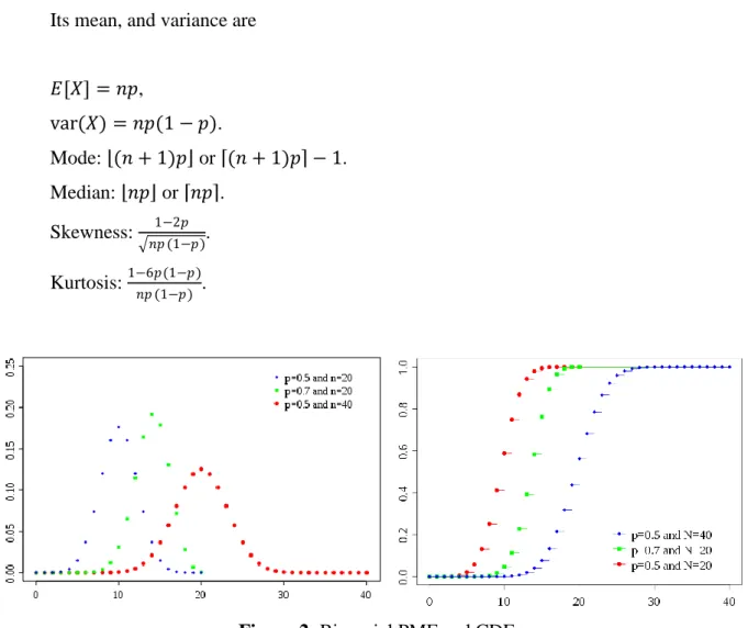
Its mean, and variance are
𝐸[𝑋] = 𝑛𝑝,
var(𝑋) = 𝑛𝑝(1 − 𝑝).
Mode: (𝑛 + 1)𝑝 or (𝑛 + 1)𝑝 − 1.
Median: 𝑛𝑝 or 𝑛𝑝 .
Skewness: 𝑛𝑝 (1−𝑝)1−2𝑝 . Kurtosis: 1−6𝑝(1−𝑝)𝑛𝑝 (1−𝑝) .
Figure 2: Binomial PMF and CDF
The binomial distribution is of repeated use each time a trial involves superposing
independent elementary trials. In the field of traffic, the Engset problem introduces it as a
The binomial distribution enjoys the following property, concerning the sum of several
variables:
THEOREM. If two discrete random variables 𝑋 and 𝑌 have binomial distributions with
parameters respectively (𝑁, 𝑝) and (𝑀, 𝑝), the variable 𝑋 + 𝑌 has a binomial distribution with
parameters (𝑁 + 𝑀, 𝑝).
1.4 The multinomial distribution
This is the generalization of the binomial law. Assume that 𝑚 types can be distinguished
in the population, so that the population has a proportion 𝑝𝑘 of elements of type 𝑘 (with naturally
𝑝𝑘 = 1). The question is: what is the probability of observing, when extracting 𝑁 items, 𝑛1 of the type 1, etc., 𝑛𝑚 of type 𝑚, with 𝑛1+ 𝑛2+. . . +𝑛𝑚 = 𝑁. The result is:
𝑃 𝑛1, 𝑛2, … , 𝑛𝑚 =𝑛 𝑁! 1!𝑛2!…𝑛𝑚!𝑝1
𝑛1 ∙ 𝑝
2𝑛2∙ … ∙ 𝑝𝑚𝑛𝑚.
This result has numerous applications. Imagine for instance observing a network element
(e.g. a concentrator) to which various sources are connected. What is the distribution of the
traffic the sources generate? Individual traffic intensity, expressed in erlangs, is distributed
between 0 and 1. One usually defines categories, according to the type of subscriber
(professional, residential, in urban area, etc.), corresponding to traffic intensities. With two
categories, the binomial distribution gives the answer. For several categories (typically: less than
0.03, between 0.03 and 0.05, ..., higher than 0.12), the distribution of the number of customers
among the categories is given by the multinomial law. Finally, knowing the distribution of the
different customers among the categories allows dimensioning the subscriber concentrator, using
the multinomial distribution. More generally, this result holds whenever a population, composed
with different sub-populations, is observed.
2 The Poisson Random Variable
A Poisson random variable takes nonnegative integer values. Its PMF is given by
𝑝𝑋(𝑘) = 𝑒−𝜆 𝜆
𝑘
where 𝜆 is a positive parameter characterizing the PMF, see Fig. 3. It is a legitimate PMF
because
𝑒−𝜆 𝜆𝑘 𝑘! ∞
𝑘=0 = 𝑒−𝜆 1 + 𝜆 +𝜆
2
2!+ 𝜆3
3! + ⋯ = 𝑒
−𝜆𝑒𝜆 = 1.
To get a feel for the Poisson random variable, think of a binomial random variable with
very small 𝑝and very large 𝑛. For example, consider the number of typos in a book with a total
of 𝑛 words, when the probability 𝑝 that any one word is misspelled is very small (associate a
word with a coin toss which comes a head when the word is misspelled), or the number of cars
involved in accidents in a city on a given day (associate a car with a coin toss which comes a
head when the car has an accident). Such a random variable can be well-modeled as a Poisson
random variable.
More precisely, the Poisson PMF with parameter 𝜆 is a good approximation for a
binomial PMF with parameters 𝑛 and 𝑝, provided 𝜆 = 𝑛𝑝, 𝑛 is very large, and 𝑝 is very small,
i.e.,
𝑒−𝜆 𝜆𝑘 𝑘! ≈
𝑛!
(𝑛−𝑘)!𝑘!𝑝𝑘(1 − 𝑝)𝑛−𝑘, 𝑘 = 0, 1, … , 𝑛.
In this case, using the Poisson PMF may result in simpler models and calculations. For
example, let 𝑛 = 100 and 𝑝 = 0.01. Then the probability of 𝑘 = 5 successes in 𝑛 = 100 trials is
calculated using the binomial PMF as
100!
95!5!0.015(1 − 0.01)95 = 0.00290.
Using the Poisson PMF with 𝜆 = 𝑛𝑝 = 100 ∙ 0.01 = 1, this probability is approximated
by
𝑒−1 1
Figure 3: The PMF 𝑒−𝜆 𝜆
𝑘
𝑘! of the Poisson random variable for different values of 𝜆. Note that if
𝜆 < 1, then the PMF is monotonically decreasing, while if 𝜆 > 1, the PMF first increases and
then decreases as the value of 𝑘increases.
The mean of the Poisson PMF can be calculated is follows:
𝐸 𝑋 = 𝑘𝑒−𝜆 𝜆𝑘
𝑘! ∞
𝑘=0 = 𝑘𝑒−𝜆 𝜆
𝑘
𝑘! ∞
𝑘=1
𝑡𝑒 𝑘=0 𝑡𝑒𝑟𝑚 𝑖𝑠 𝑧𝑒𝑟𝑜
= 𝜆 𝑒−𝜆 𝜆𝑘−1
𝑘−1 ! ∞
𝑘=1 = 𝜆 𝑒−𝜆 𝜆
𝑚
𝑚 ! ∞
𝑚=0
𝑙𝑒𝑡 𝑚=𝑘−1
= 𝜆.
The last equality is obtained by noting that 𝑒−𝜆 𝜆
𝑚
𝑚 ! ∞
𝑚 =0 = ∞𝑚=0𝑝𝑋(𝑚)= 1 is the
normalization property for the Poisson PMF.
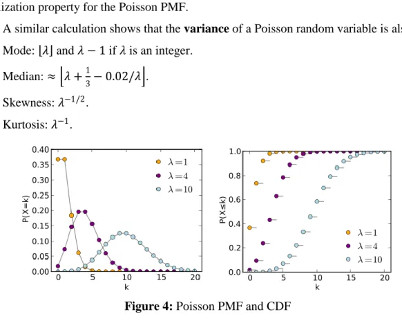
A similar calculation shows that the variance of a Poisson random variable is also 𝜆.
Mode: 𝜆 and 𝜆 − 1 if 𝜆 is an integer.
Median: ≈ 𝜆 +13− 0.02/𝜆 . Skewness: 𝜆−1/2.
Kurtosis: 𝜆−1.
Figure 4: Poisson PMF and CDF
THEOREM. Let 𝑋 and 𝑌 be two Poisson variables with parameters respectively 𝜆 and 𝜇.
3 Simplest flow of events (simple arrival)
Stemming from probability theory its application to the field of telecommunications for
the solving of traffic problems has given rise to a well-known discipline: teletraffic.
A stochastic process is a mathematical model of a probabilistic experiment that evolves
in time and generates a sequence of numerical values. For example, a stochastic process can be
used to model:
(a) the sequence of daily prices of a stock;
(b) the sequence of scores in a football game;
(c) the sequence of failure times of a machine;
(d) the sequence of hourly traffic loads at a node of a communication network;
(e) the sequence of radar measurements of the position of an airplane.
Each numerical value in the sequence is modeled by a random variable, so a stochastic
process is simply a (finite or infinite) sequence of random variables and does not represent a
major conceptual departure from our basic framework. We are still dealing with a single basic
experiment that involves outcomes governed by a probability law, and random variables that
inherit their probabilistic properties from that law.
3.1 Flow of events
Suppose that in a time line randomly arise points – moments of appearance of some
homogeneous events (for example, calls on the telephone station etc). Sequence of those
moments is so called flow of events.
Figure 5
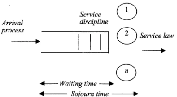
Figure 7: The basic service station
A lot of arrival processes can be described as so called Bernoulli and Poisson processes.
3.2 Arrival process
To advance in the study of traffic properties, it is necessary to look at the two components
on which it depends, i.e. client arrivals and their service.
Arrivals of clients at the system input are observed. To describe the phenomenon, the
arrival law, the first idea is to use the time interval between successive arrivals (inter-arrival
time), or the number of arrivals in a given time interval.
During the time 𝑇, 𝑛(𝑇)arrivals occur. The flow intensity is then expressed as a number, the arrival rate, whose intuitive definition is:
𝜆 = lim𝑇→∞𝑛 𝑇 𝑇 .
It is then also possible to estimate the average interval between arrivals, this being the
inverse of the previous quantity.
Figure 7 illustrates random arrivals. Consider random arrivals in the time interval from 𝑡1 to 𝑡2. The interval length is 𝑇 = 𝑡2 − 𝑡1. The arrival rate is a long term average of the number of arrivals per unit time. Its mathematical symbol is 𝜆 and its unit is 𝑡𝑖𝑚𝑒−1, and is given by the following equation, where 𝑛is the number of arrivals in the interval of length 𝑇:
𝜆 =𝑛𝑇.
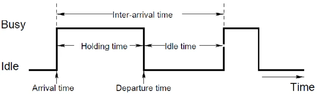
Figure 8: Illustration of the terminology applied for a traffic process. Notice the difference
between time intervals and instants of time. We use the terms arrival and call synonymously. The
inter-arrival time, respectively the inter-departure time, are the time intervals between arrivals,
respectively departures.
Flow of events is called the simplest flow if it has the properties of Poisson arrival.
3.3 The Poisson process
The Poisson process can be viewed as a continuous-time analog of the Bernoulli process
and applies to situations where there is no natural way of dividing time into discrete periods.
We consider an arrival process that evolves in continuous time, in the sense that any real
number 𝑡is a possible arrival time. We define
𝑃(𝑘, 𝜏) = 𝑃(𝑡𝑒𝑟𝑒 𝑎𝑟𝑒 𝑒𝑥𝑎𝑐𝑡𝑙𝑦 𝑘 𝑎𝑟𝑟𝑖𝑣𝑎𝑙𝑠 𝑑𝑢𝑟𝑖𝑛𝑔 𝑎𝑛 𝑖𝑛𝑡𝑒𝑟𝑣𝑎𝑙 𝑜𝑓 𝑙𝑒𝑛𝑔𝑡 𝜏),
and assume that this probability is the same for all intervals of the same length 𝜏. We also
introduce a positive parameter 𝜆to be referred to as the arrival rate or intensity of the process.
Definition of the Poisson Process
An arrival process is called a Poisson process with rate 𝜆 if it has the following
properties:
(a) (Time-homogeneity.) The probability 𝑃(𝑘, 𝜏) of 𝑘 arrivals is the same for all
intervals of the same length 𝜏.
(b) (Independence.) The number of arrivals during a particular interval is independent of
the history of arrivals outside this interval.
(c) (Small interval probabilities.) The probabilities 𝑃(𝑘, 𝜏) satisfy
𝑃(1, 𝜏) = 𝜆𝜏 + 𝑜1(𝜏).
Here, 𝑜(𝜏) and 𝑜1(𝜏) are functions of 𝜏that satisfy
lim𝜏→0𝑜(𝜏)𝜏 = 0, lim𝜏→0𝑜1𝜏(𝜏)= 0.
The first property states that arrivals are “equally likely” at all times. The arrivals during
any time interval of length 𝜏 are statistically the same, in the sense that they obey the same
probability law.
To interpret the second property, consider a particular interval [𝑡, 𝑡′], of length 𝑡′ − 𝑡.
The unconditional probability of 𝑘arrivals during that interval is 𝑃(𝑘, 𝑡′ − 𝑡). Suppose now that
we are given complete or partial information on the arrivals outside this interval. Property (b)
states that this information is irrelevant: the conditional probability of 𝑘 arrivals during [𝑡, 𝑡′]
remains equal to the unconditional probability 𝑃(𝑘, 𝑡′ − 𝑡).
The third property is critical. The 𝑜(𝜏) and 𝑜1(𝜏) terms are meant to be negligible in comparison to 𝜏 , when the interval length 𝜏 is very small. They can be thought of as the 𝑂(𝜏2) terms in a Taylor series expansion of 𝑃(𝑘, 𝜏). Thus, for small 𝝉, the probability of a single
arrival is roughly 𝝀𝝉, plus a negligible term. Similarly, for small 𝝉, the probability of zero arrivals is roughly 𝟏 − 𝝀𝝉.
Note that the probability of two or more arrivals is
1 − 𝑃(0, 𝜏) − 𝑃(1, 𝜏) = −𝑜(𝜏) − 𝑜1(𝜏),
and is negligible in comparison to 𝑃(1, 𝜏) as 𝜏gets smaller and smaller.
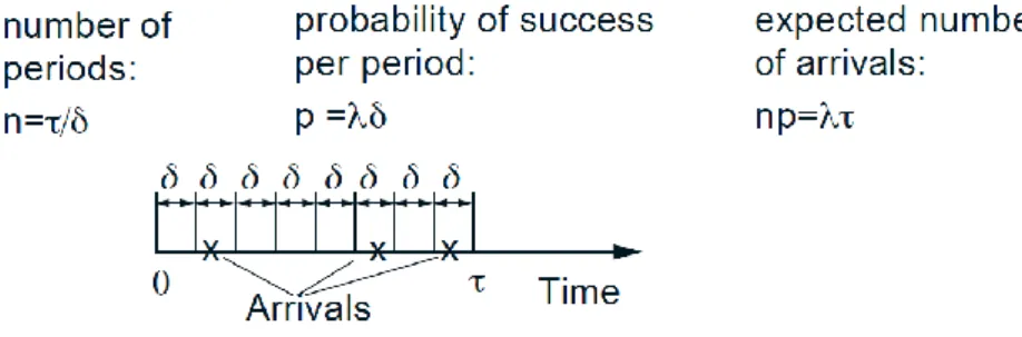
Figure 9: Bernoulli approximation of the Poisson process
Let us now start with a fixed time interval of length 𝜏 and partition it into 𝜏/𝛿 periods of
during any period can be neglected, because of property (c) and the preceding discussion.
Different periods are independent, by property (b). Furthermore, each period has one arrival with
probability approximately equal to 𝜆𝛿, or zero arrivals with probability approximately equal to
1 − 𝜆𝛿. Therefore, the process being studied can be approximated by a Bernoulli process, with
the approximation becoming more and more accurate the smaller 𝛿 is chosen. Thus the
probability 𝑃(𝑘, 𝜏) of 𝑘 arrivals in time 𝜏, is approximately the same as the (binomial)
probability of 𝑘 successes in 𝑛 = 𝜏/𝛿 independent Bernoulli trials with success probability
𝑝 = 𝜆𝛿 at each trial. While keeping the length 𝜏 of the interval fixed, we let the period length 𝛿
decrease to zero. We then note that the number 𝑛 of periods goes to infinity, while the product
𝑛𝑝 remains constant and equal to 𝜆𝜏. Under these circumstances, we can see that the binomial
PMF converges to a Poisson PMF with parameter 𝜆𝜏. We are then led to the important
conclusion that
𝑃 𝑘, 𝜏 =(𝜆𝜏 )𝑘!𝑘𝑒−𝜆𝜏, 𝑘 = 0, 1, ….
Note that a Taylor series expansion of 𝑒−𝜆𝜏, yields
𝑃(0, 𝜏) = 𝑒−𝜆𝜏 = 1 − 𝜆𝜏 + 𝑂(𝜏2),
𝑃(1, 𝜏) = 𝜆𝜏𝑒−𝜆𝜏 = 𝜆𝜏 − 𝜆2𝜏2 + 𝑂(𝜏3) = 𝜆𝜏 + 𝑂(𝜏2),
consistent with property (c).
Using our earlier formulas for the mean and variance of the Poisson PMF, we obtain
𝐸[𝑁𝜏] = 𝜆𝜏, var(𝑁𝜏) = 𝜆𝜏,
where 𝑁𝜏 stands for the number of arrivals during a time interval of length 𝜏. These formulas are hardly surprising, since we are dealing with the limit of a binomial PMF with parameters
𝑛 = 𝜏/𝛿, 𝑝 = 𝜆𝛿, mean 𝑛𝑝 = 𝜆𝜏, and variance 𝑛𝑝(1 − 𝑝) ≈ 𝑛𝑝 = 𝜆𝜏.
Let us now derive the probability law for the time 𝑇of the first arrival, assuming that the
process starts at time zero. Note that we have 𝑇 > 𝑡if and only if there are no arrivals during the
interval [0, 𝑡]. Therefore,
We then differentiate the CDF 𝐹𝑇(𝑡) of 𝑇, and obtain the PDF formula
𝑓𝑇(𝑡) = 𝜆𝑒−𝜆𝑡, 𝑡 ≥ 0,
which shows that the time until the first arrival is exponentially distributed with parameter 𝜆. We
summarize this discussion in the table that follows. See also Fig. 9.
Random Variables Associated with the Poisson Process and their Properties
The Poisson with parameter 𝝀𝝉. This is the number 𝑁𝜏 of arrivals in a Poisson
process with rate 𝜆, over an interval of length 𝜏. Its PMF, mean, and variance are
𝑝𝑁𝜏(𝑘) = 𝑃 𝑘, 𝜏 = (𝜆𝜏 )𝑘!𝑘𝑒−𝜆𝜏, 𝑘 = 0, 1, …,
𝐸[𝑁𝜏] = 𝜆𝜏, var(𝑁𝜏) = 𝜆𝜏.
The exponential with parameter 𝝀. This is the time 𝑇until the first arrival. Its PDF,
mean, and variance are
𝑓𝑇(𝑡) = 𝜆𝑒−𝜆𝑡, 𝑡 ≥ 0, 𝐸 𝑇 = 1
𝜆, var 𝑇 = 1 𝜆2.
Figure 10: View of the Bernoulli process as the discrete-time version of the Poisson. We
discretize time in small intervals 𝛿and associate each interval with a Bernoulli trial whose