Cite this:Energy Environ. Sci.,
2015,8, 2093
100% clean and renewable wind, water, and
sunlight (WWS) all-sector energy roadmaps for
the 50 United States
†
Mark Z. Jacobson,*aMark A. Delucchi,bGuillaume Bazouin,aZack A. F. Bauer,a Christa C. Heavey,aEmma Fisher,aSean B. Morris,aDiniana J. Y. Piekutowski,a Taylor A. Vencillaand Tim W. Yeskooa
This study presents roadmaps for each of the 50 United States to convert their all-purpose energy systems (for electricity, transportation, heating/cooling, and industry) to ones powered entirely by wind, water, and sunlight (WWS). The plans contemplate 80–85% of existing energy replaced by 2030 and 100% replaced by 2050. Con-version would reduce each state’s end-use power demand by a mean ofB39.3% withB82.4% of this due to the efficiency of electrification and the rest due to end-use energy efficiency improvements. Year 2050 end-use U.S. all-purpose load would be met withB30.9% onshore wind, B19.1% offshore wind,B30.7% utility-scale photovoltaics (PV),B7.2% rooftop PV,B7.3% concentrated solar power (CSP) with storage,B1.25% geothermal power,B0.37% wave power,B0.14% tidal power, andB3.01% hydroelectric power. Based on a parallel grid integration study, an additional 4.4% and 7.2% of power beyond that needed for annual loads would be supplied by CSP with storage and solar thermal for heat, respectively, for peaking and grid stability. Over all 50 states, converting would provideB3.9 million 40-year construction jobs andB2.0 million 40-year operation jobs for the energy facilities alone, the sum of which would outweigh theB3.9 million jobs lost in the conventional energy sector. Converting would also eliminateB62 000 (19 000–115 000) U.S. air pollution premature morta-lities per year today andB46 000 (12 000–104 000) in 2050, avoidingB$600 ($85–$2400) bil. per year (2013 dollars) in 2050, equivalent toB3.6 (0.5–14.3) percent of the 2014 U.S. gross domestic product. Converting would further eliminateB$3.3 (1.9–7.1) tril. per year in 2050 global warming costs to the world due to U.S. emissions. These plans will result in each person in the U.S. in 2050 savingB$260 (190–320) per year in energy costs ($2013 dollars) and U.S. health and global climate costs per person decreasing byB$1500 (210–6000) per year andB$8300 (4700–17 600) per year, respectively. The new footprint over land required will beB0.42% of U.S. land. The spacing area between wind turbines, which can be used for multiple purposes, will beB1.6% of U.S. land. Thus, 100% conversions are technically and economically feasible with little downside. These roadmaps may therefore reduce social and political barriers to implementing clean-energy policies.
Broader context
This paper presents a consistent set of roadmaps for converting the energy infrastructures of each of the 50 United States to 100% wind, water, and sunlight (WWS) for all purposes (electricity, transportation, heating/cooling, and industry) by 2050. Such conversions are obtained by first projecting conventional power demand to 2050 in each sector then electrifying the sector, assuming the use of some electrolytic hydrogen in transportation and industry and applying modest end-use energy efficiency improvements. Such state conversions may reduce conventional 2050 U.S.-averaged power demand byB39%, with most reductions due to the efficiency of electricity over combustion and the rest due to modest end-use energy efficiency improvements. The conversions are found to be technically and economically feasible with little downside. They nearly eliminate energy-related U.S. air pollution and climate-relevant emissions and their resulting health and environmental costs while creating jobs, stabilizing energy prices, and minimizing land requirements. These benefits have not previously been quantified for the 50 states. Their elucidation may reduce the social and political barriers to implementing clean-energy policies for replacing conventional combustible and nuclear fuels. Several such policies are proposed herein for each energy sector.
1. Introduction
This paper presents a consistent set of roadmaps to convert each of the 50 U.S. states’ all-purpose (electricity, transportation, aAtmosphere/Energy Program, Dept. of Civil and Env. Engineering,
Stanford University, USA. E-mail: [email protected]; Fax:+1-650-723-7058; Tel:+1-650-723-6836
bInstitute of Transportation Studies, U.C. Berkeley, USA
†Electronic supplementary information (ESI) available. See DOI: 10.1039/c5ee01283j
Received 25th April 2015, Accepted 27th May 2015 DOI: 10.1039/c5ee01283j
www.rsc.org/ees
Energy &
Environmental
Science
heating/cooling, and industry) energy infrastructures to ones powered 100% by wind, water, and sunlight (WWS). Existing energy plans in many states address the need to reduce greenhouse gas emissions and air pollution, keep energy prices low, and foster job creation. However, in most if not all states these goals are limited to partial emission reductions by 2050 (see, for example,1for a review
of California roadmaps), and no set of consistently-developed roadmaps exist for every U.S. state. By contrast, the roadmaps here provide a consistent set of pathways to eliminate 100% of present-day greenhouse gas and air pollutant emissions from energy by 2050 in all 50 sates while growing the number of jobs and stabilizing energy prices. A separate study2 provides a grid integration analysis to examine the ability of the intermittent energy produced from the state plans here, in combination, to match time-varying electric and thermal loads when combined with storage and demand response.
The methods used here to create each state roadmap are broadly similar to those recently developed for New York,3 California,4 and the world as a whole.5–7 Such methods are
applied here to make detailed, original, state-by-state estimates of (1) Future energy demand (load) in the electricity, trans-portation, heating/cooling, and industrial sectors in both a business-as-usual (BAU) case and a WWS case;
(2) The numbers of WWS generators needed to meet the estimated load in each sector in the WWS case;
(3) Footprint and spacing areas needed for WWS generators; (4) Rooftop areas and solar photovoltaic (PV) installation potentials over residential and commercial/government build-ings and associated carports, garages, parking lots, and parking structures;
(5) The levelized cost of energy today and in 2050 in the BAU and WWS cases;
(6) Reductions in air-pollution mortality and associated health costs today based on pollution data from all monitoring stations in each state and in 2050, accounting for future reduc-tions in emissions in the BAUversusWWS cases;
(7) Avoided global-warming costs today and in 2050 in the BAUversusWWS cases; and
(8) Numbers of jobs produced and lost and the resulting revenue changes between the BAU and WWS cases.
This paper further provides a transition timeline, energy efficiency measures, and potential policy measures to implement the plans. In sum, whereas, many studies focus on changing energy sources in one energy sector, such as electricity, this study integrates changes among all energy sectors: electricity, trans-portation, heating/cooling, and industry. It further provides rigorous and detailed and consistent estimates of 2050 state-by-state air pollution damage, climate damage, energy cost, solar rooftop potential, and job production and loss not previously available.
2. WWS technologies
This study assumes all energy sectors are electrified by 2050. The WWS energy technologies chosen to provide electricity include wind, concentrated solar power (CSP), geothermal, solar PV,
tidal, wave, and hydroelectric power. These generators are existing technologies that were found to reduce health and climate impacts the most among multiple technologies while minimizing land and water use and other impacts.8
The technologies selected for ground transportation, which will be entirely electrified, include battery electric vehicles (BEVs) and hydrogen fuel cell (HFC) vehicles, where the hydrogen is produced by electrolysis. BEVs with fast charging or battery swapping will dominate long-distance, light-duty transportation; Battery electric-HFC hybrids will dominate heavy-duty trans-portation and long-distance shipping; batteries will power short-distance shipping (e.g., ferries); and electrolytic cryogenic hydrogen, with batteries for idling, taxiing, and internal power, will power aircraft.
Air heating and cooling will be electrified and powered by electric heat pumps (ground-, air-, or water-source) and some electric-resistance heating. Water will be heated by heat pumps with electric resistance elements and/or solar hot water pre-heating. Cook stoves will have either an electric induction or resistance-heating element.
High-temperature industrial processes will be powered by electric arc furnaces, induction furnaces, dielectric heaters, and resistance heaters and some combusted electrolytic hydrogen. HFCs will be used only for transportation, not for electric power generation due to the inefficiency of that application for HFCs. Although electrolytic hydrogen for transportation is less efficient and more costly than is electricity for BEVs, some segments of transportation (e.g., long-distance ships and freight) may benefit from HFCs.
The roadmaps presented here include energy efficiency measures but not nuclear power, coal with carbon capture, liquid or solid biofuels, or natural gas, as previously discussed.3,6 Biofuels, for example, are not included because their combus-tion produces air pollucombus-tion at rates on the same order as fossil fuels and their lifecycle carbon emissions are highly uncertain but definitely larger than those of WWS technologies. Several biofuels also have water and land requirements much larger than those of WWS technologies. Since photosynthesis is 1% efficient whereas solar PV, for example, isB20% efficient, the same land used for PV producesB20 times more energy than does using the land for biofuels.
This study first calculates the installed capacity and number of generators of each type needed in each state to potentially meet the state’sannualpower demand (assuming state-specific average-annual capacity factors) in 2050 after all sectors have been electrified, without considering sub-annual (e.g., daily or hourly) load balancing. The calculations assume only that existing hydroelectric from outside of a state continues to come from outside. The study then provides the additional number of generators needed by state to ensure that hourly power demand across all states does not suffer loss of load, based on results from ref. 2. As such, while the study bases each state’s installed capacity on the state’s annual demand, it allows interstate transmission of power as needed to ensure that supply and demand balance every hour in every state. We also roughly estimate the additional cost of transmission lines needed for
this hourly balancing. Note that if we relax our assumption that each state’s capacity match its annual demand, and instead allow states with especially good solar or wind resources to have enough capacity to supply larger regions, then the average levelized cost of electricity will be lower than we estimate because of the higher average capacity factors in states with the best WWS resources.
3. Changes in U.S. power load upon
conversion to WWS
Table 1 summarizes the state-by-state end-use load calculated by sector in 2050 if conventional fuel use continues along BAU or ‘‘conventional energy’’ trajectory. It also shows the estimated new load upon a conversion to a 100% WWS infrastructure (with zero fossil fuels, biofuels, or nuclear fuels). The table is derived from a spreadsheet analysis of annually averaged end-use load data.9All end uses that feasibly can be electrified are
assumed to use WWS power directly, and remaining end uses (some heating, high-temperature industrial processes, and some transportation) are assumed to use WWS power indirectly in the form of electrolytic hydrogen (hydrogen produced by splitting water with WWS electricity). End-use power excludes losses incurred during production and transmission of the power.
With these roadmaps, electricity generation increases, but the use of oil and gas for transportation and heating/cooling decreases to zero. Further, the increase in electricity use due to electrifying all sectors is much less than the decrease in energy in the gas, liquid, and solid fuels that the electricity replaces, because of the high energy-to-work conversion efficiency of electricity used for heating and electric motors. As a result, end use load decreases significantly with WWS energy systems in all 50 states (Table 1).
In 2010, U.S. all-purpose, end-use load was B2.37 TW (terawatts, or trillion watts). Of this, 0.43 TW (18.1%) was electric power load. If the U.S. follows the business-as-usual (BAU) trajectory of the current energy infrastructure, which involves growing load and modest shifts in the power sector away from coal to renewables and natural gas, all-purpose end-use load is expected to grow to 2.62 TW in 2050 (Table 1).
A conversion to WWS by 2050 is calculated here to reduce U.S. end-use load and the power required to meet that load by
B39.3% (Table 1). About 6.9 percentage points of this reduction is due to modest additional energy-conservation measures (Table 1, last column) and another relatively small portion is due to the fact that conversion to WWS reduces the need for energy use in petroleum refining. The remaining and major reason for the reduction is that the use of electricity for heating and electric motors is more efficient than is fuel combustion for the same applications.6 Also, the use of WWS electricity to produce hydrogen for fuel cell vehicles, while less efficient than the use of WWS electricity to run BEVs, is more efficient and cleaner than is burning liquid fossil fuels for vehicles.6,10 Combusting electrolytic hydrogen is slightly less efficient but cleaner than is combusting fossil fuels for direct heating,
and this is accounted for in Table 1. In Table 1,B11.48% of all 2050 WWS electricity (47.8% of transportation load, and 5.72% of industrial load) will be used to produce, store, and use hydrogen, for long distance and heavy transportation and some high-temperature industrial processes.
The percent decrease in load upon conversion to WWS in Table 1 is greater in some states (e.g., Hawaii, California, Florida, New Jersey, New Hampshire, and Vermont) than in others (e.g. Minnesota, Iowa, and Nebraska). The reason is that the transportation-energy share of the total in the states with the large reductions is greater than in those with the small reduc-tions, and efficiency gains from electrifying transportation are much greater than are efficiency gains from electrifying other sectors.
4. Numbers of electric power
generators needed and land-use
implications
Table 2 summarizes the number of WWS power plants or devices needed to power each U.S. state in 2050 for all purposes assuming end use power requirements in Table 1, the percent mix of end-use power generation in Table 3, and electrical transmission, distribution, and array losses. The specific mix of generators presented for each state in Table 3 is just one set of options.
Rooftop PV in Table 2 is divided into residential (5 kW systems on average) and commercial/government (100 kW systems on average). Rooftop PV can be placed on existing rooftops or on elevated canopies above parking lots, highways, and structures without taking up additional undeveloped land. Table 4 sum-marizes projected 2050 rooftop areas by state usable for solar PV on residential and commercial/government buildings, carports, garages, parking structures, and parking lot canopies. The rooftop areas in Table 4 are used to calculate potential rooftop generation, which in turn limits the penetration of residential and commercial/government PV in Table 3. Utility-scale PV power plants are sized, on average, relatively small (50 MW) to allow them to be placed optimally in available locations. While utility-scale PV can operate in any state because it can take advantage of both direct and diffuse solar radiation, CSP is assumed to be viable only in states with sufficient direct solar radiation. While some states listed in Table 3, such as states in the upper Midwest, are assumed to install CSP although they have marginal average solar insolation, such states have regions with greater than average insolation, and the value of CSP storage is sufficiently high to suggest a small penetration of CSP in those states.
Onshore wind is assumed to be viable primarily in states with good wind resources (Section 5.1). Offshore wind is assumed to be viable offshore of any state with either ocean or Great Lakes coastline (Section 5.1). Wind and solar are the only two sources of electric power with sufficient resource to power the whole U.S. independently on their own. Averaged over the U.S., wind (B50.0%) and solar (45.2%) are the largest generators of
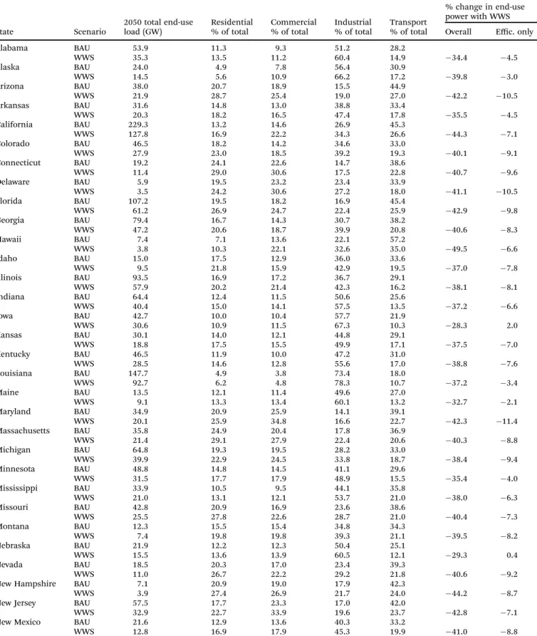
Table 1 1st row of each state: estimated 2050 total end-use load (GW) and percent of total load by sector if conventional fossil-fuel, nuclear, and biofuel use continue from today to 2050 under a business-as-usual (BAU) trajectory. 2nd row of each state: estimated 2050 total end-use load (GW) and percent of total load by sector if 100% of BAU end-use all-purpose delivered load in 2050 is instead provided by WWS. The estimate in the ‘‘% change’’ column for each state is the percent reduction in total 2050 BAU load due to switching to WWS, including (second-to-last column) the effects of assumed policy-based improvements in end-use efficiency, inherent reductions in energy use due to electrification, and the elimination of energy use for the upstream production of fuels (e.g., petroleum refining). The number in the last column is the reduction due only to assumed, policy-driven end-use energy efficiency measuresa
State Scenario
2050 total end-use load (GW)
Residential % of total
Commercial % of total
Industrial % of total
Transport % of total
% change in end-use power with WWS Overall Effic. only
Alabama BAU 53.9 11.3 9.3 51.2 28.2
WWS 35.3 13.5 11.2 60.4 14.9 34.4 4.5
Alaska BAU 24.0 4.9 7.8 56.4 30.9
WWS 14.5 5.6 10.9 66.2 17.2 39.8 3.0
Arizona BAU 38.0 20.7 18.9 15.5 44.9
WWS 21.9 28.7 25.4 19.0 27.0 42.2 10.5
Arkansas BAU 31.6 14.8 13.0 38.8 33.4
WWS 20.3 18.2 16.5 47.4 17.8 35.5 4.5
California BAU 229.3 13.2 14.6 26.9 45.3
WWS 127.8 16.9 22.2 34.3 26.6 44.3 7.1
Colorado BAU 46.5 18.2 14.2 34.6 33.0
WWS 27.9 23.0 18.5 39.2 19.3 40.1 9.1
Connecticut BAU 19.2 24.1 22.6 14.7 38.6
WWS 11.4 29.0 30.6 17.5 22.8 40.7 9.6
Delaware BAU 5.9 19.5 23.2 23.4 33.9
WWS 3.5 24.2 30.6 27.2 18.0 41.1 10.5
Florida BAU 107.2 19.5 18.2 16.9 45.4
WWS 61.2 26.9 24.7 22.4 25.9 42.9 9.8
Georgia BAU 79.4 16.7 14.3 30.7 38.2
WWS 47.2 20.6 18.7 39.9 20.8 40.6 8.3
Hawaii BAU 7.4 7.1 13.6 22.1 57.2
WWS 3.8 10.3 22.1 32.6 35.0 49.5 6.6
Idaho BAU 15.0 17.5 12.9 36.0 33.6
WWS 9.5 21.8 15.9 42.9 19.5 37.0 7.8
Illinois BAU 93.5 16.9 17.2 36.7 29.1
WWS 57.9 20.2 21.4 42.3 16.2 38.1 8.1
Indiana BAU 64.4 12.4 11.5 50.6 25.6
WWS 40.4 15.0 14.1 57.5 13.5 37.2 6.6
Iowa BAU 42.7 10.0 10.4 57.7 21.9
WWS 30.6 10.9 11.5 67.3 10.3 28.3 2.0
Kansas BAU 30.1 14.0 12.1 44.8 29.1
WWS 18.8 17.5 15.5 49.9 17.1 37.5 7.0
Kentucky BAU 46.5 11.9 10.0 47.2 31.0
WWS 28.5 14.6 12.8 55.6 17.0 38.8 7.6
Louisiana BAU 147.7 4.9 3.8 73.4 18.0
WWS 92.7 6.2 4.8 78.3 10.7 37.2 3.4
Maine BAU 13.5 12.1 11.4 49.6 27.0
WWS 9.1 13.3 13.4 60.1 13.2 32.7 2.1
Maryland BAU 34.9 20.9 25.9 14.1 39.1
WWS 20.1 25.9 34.8 16.6 22.7 42.3 11.4
Massachusetts BAU 35.8 24.9 20.4 17.8 36.9
WWS 21.4 29.1 27.9 22.4 20.6 40.3 8.8
Michigan BAU 64.8 19.3 19.5 28.2 33.0
WWS 39.9 22.9 24.5 33.8 18.7 38.4 9.4
Minnesota BAU 48.8 14.8 14.5 41.1 29.6
WWS 31.5 17.7 17.9 48.9 15.5 35.4 4.0
Mississippi BAU 33.9 10.5 9.5 44.1 35.8
WWS 21.0 13.1 12.1 53.7 21.0 38.0 6.3
Missouri BAU 42.8 20.9 16.9 23.6 38.6
WWS 25.5 27.8 22.6 28.7 21.0 40.4 7.3
Montana BAU 12.3 15.5 15.4 34.8 34.3
WWS 7.4 19.8 19.8 39.3 21.1 39.5 8.2
Nebraska BAU 21.9 12.2 12.3 50.4 25.1
WWS 15.5 13.6 13.9 60.5 12.1 29.3 0.4
Nevada BAU 18.5 20.3 17.0 23.4 39.3
WWS 11.0 26.7 22.2 29.2 21.8 40.6 9.2
New Hampshire BAU 7.1 20.9 19.0 17.9 42.3
WWS 3.9 27.4 26.9 21.7 24.0 44.2 8.7
New Jersey BAU 57.5 17.7 23.3 17.0 42.0
WWS 32.9 22.7 33.9 19.6 23.7 42.8 7.1
New Mexico BAU 21.6 12.9 13.6 40.3 33.2
WWS 12.8 16.9 17.9 45.3 19.9 41.0 8.8
annually averaged end-use electric power under these plans. The ratio of wind to solar end-use power is 1.1 : 1.
Under the roadmaps, the 2050 installed capacity of hydro-electric, averaged over the U.S., is assumed to be virtually the same as in 2010, except for a small growth in Alaska. However, existing dams in most states are assumed to run more effi-ciently for producing peaking power, thus the capacity factor of dams is assumed to increase (Section 5.4). Geothermal, wave, and tidal energy expansions are limited in each state by their potentials (Sections 5.3, 5.5 and 5.6, respectively).
Table 2 lists installed capacities beyond those needed to match annually averaged power demand for CSP with storage and for solar thermal. These additional capacities are derived in the separate grid integration study2and are needed to produce peaking power, to account for additional loads due to losses in and out of storage, and to ensure reliability of the grid, as described and quantified in that paper.
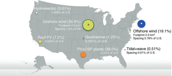
Fig. 1 shows the additional footprint and spacing areas required from Table 2 to replace the entire U.S. all-purpose energy infra-structure with WWS by 2050. Footprint area is the physical area on the ground needed for each energy device. Spacing area is the area between some devices, such as wind, tidal, and wave turbines, needed to minimize interference of the wake of one turbine with downwind turbines.
Table 2 indicates that the total new land footprint required for the plans, averaged over the U.S. isB0.42% of U.S. land area, mostly for solar PV power plants (rooftop solar does not take up new land). This does not account for the decrease in footprint from eliminating the current energy infrastructure, which includes the footprint for mining, transporting, and refining fossil fuels and uranium and for growing, transporting, and refining biofuels.
The only spacing over land needed for the WWS system is between onshore wind turbines and this requires B1.6% of U.S. land. The footprint associated with this spacing is trivial,
Table 1 (continued)
State Scenario
2050 total end-use load (GW)
Residential % of total
Commercial % of total
Industrial % of total
Transport % of total
% change in end-use power with WWS Overall Effic. only
New York BAU 86.3 23.0 30.1 15.0 31.8
WWS 54.9 26.5 39.0 16.6 17.9 36.4 7.8
North Carolina BAU 62.7 19.8 18.9 25.8 35.5
WWS 37.9 24.8 24.2 32.1 18.9 39.5 9.8
North Dakota BAU 14.3 7.3 8.7 59.0 24.9
WWS 9.0 9.1 11.0 64.4 15.5 36.9 4.6
Ohio BAU 87.0 16.2 16.4 37.6 29.8
WWS 53.5 19.8 20.5 43.6 16.1 38.5 8.2
Oklahoma BAU 47.3 13.1 11.4 41.1 34.4
WWS 29.1 16.7 15.0 47.0 21.3 38.5 6.9
Oregon BAU 27.3 15.4 15.6 26.5 42.6
WWS 16.3 18.9 21.9 34.6 24.6 40.4 8.5
Pennsylvania BAU 94.0 15.4 14.1 39.5 31.0
WWS 59.1 18.5 18.3 44.1 19.2 37.2 7.3
Rhode Island BAU 5.5 24.2 21.1 19.9 34.9
WWS 3.2 28.9 28.9 21.7 20.5 41.5 10.7
South Carolina BAU 39.7 15.1 13.0 36.3 35.6
WWS 24.2 19.0 16.6 45.8 18.6 39.1 7.8
South Dakota BAU 10.6 10.6 11.1 50.4 28.0
WWS 7.5 11.8 12.5 61.9 13.9 29.1 1.8
Tennessee BAU 52.8 15.6 13.5 36.5 34.3
WWS 32.2 19.6 17.4 44.5 18.4 39.1 7.3
Texas BAU 376.6 8.4 8.0 56.9 26.7
WWS 225.3 11.2 10.8 62.7 15.3 40.2 4.8
Utah BAU 23.2 17.8 16.6 28.7 36.8
WWS 13.8 22.8 21.8 33.0 22.4 40.6 9.1
Vermont BAU 3.7 25.1 16.3 19.2 39.4
WWS 2.1 31.8 22.4 24.3 21.5 42.7 8.6
Virginia BAU 60.3 18.0 20.3 23.1 38.6
WWS 35.1 22.7 27.1 28.5 21.7 41.8 10.2
Washington BAU 52.8 14.3 15.2 30.2 40.4
WWS 31.7 17.7 21.3 38.7 22.4 39.9 7.4
West Virginia BAU 21.7 14.3 12.3 40.6 32.7
WWS 13.0 17.0 15.9 45.3 21.7 39.9 12.3
Wisconsin BAU 41.9 15.7 17.2 39.6 27.4
WWS 26.8 18.3 20.7 47.3 13.8 36.0 6.4
Wyoming BAU 18.1 6.0 8.3 56.2 29.5
WWS 11.2 7.4 10.4 61.2 20.9 38.3 8.5
United States BAU 2621.4 14.3 14.1 38.5 33.1
WWS 1591.0 17.8 18.6 45.0 18.6 39.3 6.9
aBAU values are extrapolations from the U.S. Energy Information Administration (EIA) projections for the year 2040. WWS values are estimated with respect to BAU values accounting for the effect of electrification of end-uses on energy requirements and the effects of additional energy-efficiency measures. See the ESI and ref. 9 for details.
and the spacing area can be used for multiple purposes, such as agricultural land, grazing land, and open space. Landowners can thus derive income, not only from the wind turbines on the land, but also from farming around the turbines.
5. Resource availability
This section evaluates whether the United States has sufficient wind, solar, geothermal, and hydroelectric resources to supply the country’s all-purpose energy in 2050.
5.1. Wind
Fig. 2 shows three-dimensional computer model estimates, derived for this study, of the U.S. annually averaged capacity factor of wind turbines if they are installed onshore and off-shore. The calculations are performed assuming a REpower 5 MW turbine with a 126 m diameter rotor (the same turbine assumed for the roadmaps). Results are obtained for a hub height of 100 m above the topographical surface. Spacing areas of 4 7 rotor diameters are used for onshore turbines and 510 diameters for offshore turbines.
Table 2 Number, capacity, footprint area, and spacing area of WWS power plants or devices needed to provide total annually-averaged end-use all-purpose load over all 50 states plus additional power needed to provide peaking and storage services, as derived in ref. 2. The numbers account for short-and moderate-distance transmission, distribution, forced short-and unforced maintenance, short-and array losses. Ref. 9 derives individual tables for each state
Energy technology
Rated power one plant or device (MW)
Percent of 2050 all-purpose load met by plant/ devicea
Name-plate capacity of existing plus new plants or devices (MW) Percent name-plate capacity already installed 2013 Number of new plants or devices needed for U.S.
Percent of U.S. land area for foot-print of new plants/ devicesb Percent of U.S. land area for spacing of new plants/ devices Annual power
Onshore wind 5 30.92 1 701 000 3.59 328 000 0.00004 1.5912
Offshore wind 5 19.08 780 900 0.00 156 200 0.00002 0.7578
Wave device 0.75 0.37 27 040 0.00 36 050 0.00021 0.0098
Geothermal plant 100 1.25 23 250 10.35 208 0.00078 0.0000
Hydroelectric plantc 1300 3.01 91 650 95.87 3 0.02077 0.0000
Tidal turbine 1 0.14 8823 0.00 8823 0.00003 0.0004
Res. roof PV 0.005 3.98 379 500 0.94 75 190 000 0.03070 0.0000
Com/gov roof PVd 0.1 3.24 276 500 0.64 2 747 000 0.02243 0.0000
Solar PV plantd 50 30.73 2 326 000 0.08 46 480 0.18973 0.0000
Utility CSP plant 100 7.30 227 300 0.00 2273 0.12313 0.0000
Total 100.00 5 841 000 2.71 0.388 2.359
Peaking/storage
Additional CSPe 100 4.38 136 400 0.00 1364 0.07388 0.0000
Solar thermale 50 7.21 469 000 0.00 9380 0.00731 0.0000
Total all 6 447 000 2.46 0.469 2.359
Total new landf 0.416 1.591
The national total number of each device is the sum among all states. The number of devices in each state is the end use load in 2050 in each state (Table 1) multiplied by the fraction of load satisfied by each source in each state (Table 3) and divided by the annual power output from each device. The annual output equals the rated power (this table; same for all states) multiplied by the state-specific annual capacity factor of the device and accounting for transmission, distribution, maintenance-time, and array losses. The capacity factor is determined for each device in each state in ref. 9. The state-by-state capacity factors for onshore wind turbines in 2050, accounting for transmission, distribution, maintenance-time, and array losses, are calculated from actual 2013 state installed capacity11and power output12with an assumed increase in capacity factor between 2013 and 2050 due to turbine efficiency improvements and a decrease due to diminishing quality of sites after the best are taken. The 2050 U.S. mean onshore wind capacity factor calculated in this manner (after transmission, distribution, maintenance-time, and array losses) is 29.0%. The highest state onshore wind capacity factor in 2050 is estimated to be 40.0%, for Oklahoma; the lowest, 17.0%, for Alabama, Kentucky, Mississippi, and Tennessee. Offshore wind turbines are assumed to be placed in locations with hub-height wind speeds of 8.5 m s 1or higher,13which corresponds to a capacity factor before transmission, distribution, maintenance, and array losses ofB42.5% for the same turbine and 39.0%, in the U.S. average after losses. Short- and moderate distance transmission, distribution, and maintenance-time losses for offshore wind and all other energy sources treated here, except rooftop PV, are assumed to be 5–10%. Rooftop PV losses are assumed to be 1–2%. Wind array losses due to competition among turbines for the same energy are an additional 8.5%.2The plans assume 38 (30–45)% of onshore wind and solar and 20 (15–25)% of offshore wind is subject to long-distance transmission with line lengths of 875 (750–1000) km and 75 (50–100) km, respectively. Line losses are 4 (3–5)% per 1000 km plus 1.5 (1.3–1.8)% of power in the station equipment. Footprint and spacing areas are calculated from the spreadsheets in ref. 9. Footprint is the area on the top surface of soil covered by an energy technology, thus does not include underground structures.aTotal end-use power demand in 2050 with 100% WWS is estimated from Table 1. bTotal land area for each state is given in ref. 9. U.S. land area is 9 161 924 km2.cThe average capacity factor for hydro is assumed to increase from its current value to 52.5% (see text). For hydro already installed capacity is based on data for 2010.dThe solar PV panels used for this calculation are Sun Power E20 panels. The capacity factors used for residential and commercial/government rooftop solar production estimates are given in ref. 9 for each state. For utility solar PV plants, nominal spacing between panels is included in the plant footprint area. The capacity factors assumed for utility PV are given in ref. 9.eThe installed capacities for peaking power/storage are derived in the separate grid integration study.2Additional CSP is CSP plus storage beyond that needed for annual power generation to firm the grid across all states. Additional solar thermal is used for soil heat storage. Other types of storage are also used in ref. 2.fThe footprint area requiring new land is equal to the footprint area for new onshore wind, geothermal, hydroelectric, and utility solar PV. Offshore wind, wave, and tidal are in water, and so do not require new land. The footprint area for rooftop solar PV does not entail new land because the rooftops already exist and are not used for other purposes (that might be displaced by rooftop PV). Only onshore wind entails new land for spacing area. The other energy sources either are in water or on rooftops, or do not use additional land for spacing. Note that the spacing area for onshore wind can be used for multiple purposes, such as open space, agriculture, grazing,etc.
Results suggest a U.S. mean onshore capacity factor ofB30.5% and offshore of B37.3% before transmission, distribution, maintenance-time, and array losses (Fig. 2). Locations of strong onshore wind resources include the Great Plains, northern parts of the northeast, and many areas in the west. Weak wind regimes include the southeast and the westernmost part of the west coast continent. Strong offshore wind resources occur off the east coast north of South Carolina and the Great Lakes. Very good offshore wind resources also occur offshore the west coast and offshore the southeast and gulf coasts. Table 2 indicates that the 2050 clean-energy plans requireB1.6% of U.S. onshore land and 0.76% of U.S. onshore-equivalent land area sited offshore
for wind-turbine spacing to power 50.0% of all-purpose annually-averaged 2050 U.S. energy. The mean capacity factor before transmission, distribution, maintenance-time, and array losses used to derive the number of onshore wind turbines needed in Table 2 isB35% and for offshore turbines is 42.5% (Table 2, footnote). Fig. 2 suggests that much more land and ocean areas with these respective capacity factors or higher are available than are needed for the roadmaps.
5.2. Solar
World solar power resources are known to be large.16Here, such resources are estimated (Fig. 3) for the U.S. using a 3-D climate
Table 3 Percent of annually-averaged 2050 U.S. state all-purpose end-use load in a WWS world from Table 1 proposed here to be met by the given electric power generator. Power generation by each resource in each state is limited by resource availability, as discussed in Section 5. All rows add up to 100%
State Onshore wind Offshore wind Wave Geothermal Hydro-electric Tidal Res PV Comm/gov PV Utility PV CSP
Alabama 5.00 10.00 0.08 0.00 4.84 0.01 3.50 2.20 64.38 10.00
Alaska 50.00 20.00 1.00 7.00 14.96 1.00 0.23 0.15 5.66 0.00
Arizona 18.91 0.00 0.00 2.00 6.49 0.00 1.30 9.30 32.00 30.00
Arkansas 43.00 0.00 0.00 0.00 3.44 0.00 4.40 3.50 35.66 10.00
California 25.00 10.00 0.50 5.00 4.48 0.50 7.50 5.50 26.52 15.00
Colorado 55.00 0.00 0.00 3.00 1.24 0.00 4.20 4.00 17.56 15.00
Connecticut 5.00 45.00 1.00 0.00 0.56 0.00 4.00 3.35 41.09 0.00
Delaware 5.00 65.00 1.00 0.00 0.00 0.50 5.00 3.85 19.65 0.00
Florida 5.00 14.93 1.00 0.00 0.05 0.04 11.2 7.80 49.98 10.00
Georgia 5.00 35.00 0.30 0.00 2.27 0.08 5.50 4.30 42.55 5.00
Hawaii 12.00 16.00 1.00 30.00 0.33 1.00 14.0 9.00 9.67 7.00
Idaho 35.00 0.00 0.00 15.00 14.96 0.00 4.00 3.20 17.84 10.00
Illinois 60.00 5.00 0.00 0.00 0.03 0.00 2.85 2.90 26.22 3.00
Indiana 50.00 0.00 0.00 0.00 0.08 0.00 2.45 2.20 42.77 2.50
Iowa 68.00 0.00 0.00 0.00 0.25 0.00 1.50 1.50 25.75 3.00
Kansas 70.00 0.00 0.00 0.00 0.01 0.00 3.20 3.00 13.79 10.00
Kentucky 8.45 0.00 0.00 0.00 1.51 0.00 3.20 2.10 79.74 5.00
Louisiana 0.65 60.00 0.40 0.00 0.11 0.00 1.30 1.20 31.34 5.00
Maine 35.00 35.00 1.00 0.00 5.79 1.00 5.40 1.80 15.01 0.00
Maryland 5.00 60.00 1.00 0.00 1.53 0.03 5.40 4.80 22.24 0.00
Massachusetts 13.00 55.00 1.00 0.00 1.42 0.06 3.90 3.30 22.32 0.00
Michigan 40.00 31.00 1.00 0.00 0.69 0.00 3.50 3.20 18.61 2.00
Minnesota 60.00 19.00 0.00 0.00 3.61 0.00 2.50 3.00 9.89 2.00
Mississippi 5.00 10.00 1.00 0.00 0.00 1.00 2.40 1.60 74.00 5.00
Missouri 60.00 0.00 0.00 0.00 1.15 0.00 5.10 4.40 24.35 5.00
Montana 35.00 0.00 0.00 9.00 19.15 0.00 2.80 2.10 21.95 10.00
Nebraska 65.00 0.00 0.00 0.00 0.94 0.00 2.20 2.00 19.86 10.00
Nevada 10.00 0.00 0.00 30.00 5.02 0.00 12.0 8.00 19.23 15.75
New Hampshire 40.00 20.00 1.00 0.00 6.48 0.50 4.50 3.30 24.22 0.00
New Jersey 10.00 55.50 0.80 0.00 0.01 0.10 3.54 2.80 27.25 0.00
New Mexico 50.00 0.00 0.00 10.00 0.35 0.00 5.50 3.80 14.35 16.00
New York 10.00 40.00 0.80 0.00 6.54 0.10 3.60 3.20 35.76 0.00
North Carolina 5.00 50.00 0.75 0.00 2.69 0.03 6.00 4.00 26.53 5.00
North Dakota 55.00 0.00 0.00 0.00 2.95 0.00 1.00 1.00 35.05 5.00
Ohio 45.00 10.00 0.00 0.00 0.10 0.00 3.20 3.00 35.70 3.00
Oklahoma 65.00 0.00 0.00 0.00 1.54 0.00 3.20 2.80 17.46 10.00
Oregon 32.50 15.00 1.00 5.00 27.25 0.05 4.00 2.20 8.00 5.00
Pennsylvania 20.00 3.00 1.00 0.00 0.74 0.85 3.30 2.35 68.76 0.00
Rhode Island 10.00 63.00 1.00 0.00 0.05 0.08 4.40 3.70 17.78 0.00
South Carolina 5.00 50.00 1.00 0.00 2.90 0.30 4.00 2.80 27.70 6.30
South Dakota 61.00 0.00 0.00 0.00 11.10 0.00 1.70 1.80 14.40 10.00
Tennessee 8.00 0.00 0.00 0.00 4.26 0.00 3.50 2.20 75.04 7.00
Texas 50.00 13.90 0.10 0.50 0.16 0.00 3.00 2.50 15.84 14.00
Utah 40.00 0.00 0.00 8.00 1.03 0.00 4.00 4.00 27.97 15.00
Vermont 25.00 0.00 0.00 0.00 64.35 0.00 4.20 2.80 3.65 0.00
Virginia 10.00 50.00 0.50 0.00 1.29 0.05 4.20 3.50 25.46 5.00
Washington 35.00 13.00 0.50 0.65 35.42 0.30 2.90 1.50 10.73 0.00
West Virginia 30.00 0.00 0.00 0.00 1.14 1.00 2.50 1.70 61.66 2.00
Wisconsin 45.00 30.00 0.00 0.00 0.96 0.00 3.30 2.90 15.84 2.00
Wyoming 65.00 0.00 0.00 1.00 1.43 0.00 1.10 0.70 20.77 10.00
United States 30.92 19.08 0.37 1.25 3.01 0.14 3.98 3.24 30.73 7.30
model that treats radiative transfer accounting for sun angles, day/night, and clouds. The best solar resources in the U.S. are broadly in the Southwest, followed by the Southeast, the Northwest, then the Northeast. The land area in 2050 required for non-rooftop solar under the plan here is equivalent toB0.394% of U.S. land area, which is a small percentage of the area of strong solar resources available (Fig. 3).
The estimates of potential generation by solar rooftop PV shown in Tables 2 and 3 are based on state-by-state calculations of available roof areas and PV power potentials on residential, commercial, and governmental buildings, garages, carports, parking lots, and parking structures. Commercial and governmental buildings include all non-residential buildings except manufacturing, industrial, and military buildings. (Commercial buildings do include schools.)
Table 4 Rooftop areas suitable for PV panels, potential capacity of suitable rooftop areas, and proposed installed capacity for both residential and commercial/government buildings, by state. See ref. 9 for detailed calculations
State
Residential rooftop PV Commercial/government rooftop PV Rooftop area
suitable for PVs in 2012 (km2)
Potential capacity of suitable area in 2050 (MWdc-peak)
Proposed installed capa-city in 2050 (MWdc-peak)
Percent of potential capacity installed Rooftop area suitable for PVs in 2012 (km2)
Potential capacity of suitable area in 2050 (MWdc-peak)
Proposed installed capa-city in 2050 (MWdc-peak)
Percent of potential capacity installed
Alabama 59.7 10 130 7409 73 35.4 6150 4175 68
Alaska 7.0 760 414 54 4.2 460 242 53
Arizona 7.1 3520 1379 39 46.9 23 210 8841 38
Arkansas 36.7 7090 5217 74 27.0 5330 3720 70
California 336.1 83 150 48 412 58 220.6 55 330 31 826 58
Colorado 48.8 11 190 6684 60 40.6 9440 5706 60
Connecticut 32.2 4640 3301 71 25.1 3690 2478 67
Delaware 10.9 1940 1182 61 7.3 1320 816 62
Florida 229.1 85 950 33 873 39 148.4 55 750 21 147 38
Georgia 108.9 25 760 15 431 60 76.9 18 450 10 815 59
Hawaii 12.7 3260 2291 70 7.5 1950 1320 68
Idaho 16.2 4030 2318 58 12.2 3070 1663 54
Illinois 116.3 17 220 11 537 67 110.6 16 770 10 524 63
Indiana 65.6 10 500 6652 63 54.8 8960 5354 60
Iowa 31.2 4430 3165 71 29.4 4260 2837 67
Kansas 32.1 5220 3804 73 28.1 4680 3197 68
Kentucky 52.7 8270 6076 73 32.3 5200 3575 69
Louisiana 54.2 9910 6582 66 44.6 8350 5447 65
Maine 32.2 4740 3340 70 9.4 1410 998 71
Maryland 60.5 11 550 7102 61 49.0 9530 5659 59
Massachusetts 58.6 8560 6053 71 46.4 6930 4591 66
Michigan 105.0 14 970 10 142 68 89.0 12 980 8312 64
Minnesota 52.9 9280 5564 60 54.6 9740 5985 61
Mississippi 35.5 4950 3653 74 22.6 3230 2183 68
Missouri 72.9 12 260 8270 67 58.0 9980 6396 64
Montana 11.6 1880 1391 74 8.2 1350 936 69
Nebraska 20.5 3140 2228 71 18.0 2830 1816 64
Nevada 29.4 15 120 6451 43 18.8 9600 3855 40
New Hampshire
13.9 2480 1287 52 9.3 1680 846 50
New Jersey 83.1 12 730 8345 66 60.7 9520 5917 62
New Mexico 24.7 5070 3674 72 15.7 3300 2276 69
New York 165.2 20 140 14 545 72 135.0 16 940 11 590 68
North Carolina
119.2 28 340 14 084 50 74.6 17 950 8417 47
North Dakota 7.2 940 639 68 6.8 920 573 62
Ohio 117.0 16 960 11 623 69 101.0 15 000 9768 65
Oklahoma 46.2 8150 5544 68 34.8 6270 4349 69
Oregon 43.5 8590 4431 52 21.6 4330 2185 50
Pennsylvania 136.4 18 870 13 757 73 87.9 12 410 8782 71
Rhode Island 9.9 1460 1015 70 7.8 1180 765 65
South Carolina
58.4 9220 6057 66 36.8 5950 3801 64
South Dakota 8.5 1290 857 66 8.3 1280 813 64
Tennessee 76.6 12 020 7246 60 45.9 7370 4083 55
Texas 268.9 78 190 36 792 47 216.9 63 550 27 485 43
Utah 23.1 6360 3160 50 20.9 5810 2833 49
Vermont 7.5 1110 672 61 4.5 680 402 59
Virginia 88.1 17 400 9825 56 65.8 13 190 7339 56
Washington 73.6 14 050 6774 48 37.2 7180 3141 44
West Virginia 24.3 3140 2273 72 16.1 2140 1386 65
Wisconsin 59.5 9310 6236 67 48.3 7710 4912 64
Wyoming 6.3 1050 754 72 4.5 760 430 57
United States 3197.6 660 290 379 513 57 2386 505 070 276 508 55
Ref. 4 (Supplemental Information) and ref. 9 document how rooftop areas and generation potential are calculated for California for four situations: residential-warm, residential-cool, commercial/government-warm, and commercial/government-cool. This method is applied here to calculate potential rooftop PV generation in each state, accounting for housing units and
building areas, available solar insolation, degradation of solar panels over time, technology improvements over time, and DC to AC power conversion losses.
Each state’s potential installed capacity of rooftop PV in 2050 equals the potential alternating-current (AC) generation from rooftop PV in 2050 in the state divided by the PV capacity
Fig. 1 Spacing and footprint areas required from Table 2 for annual power load, beyond existing 2013 resources, to repower the U.S. state-by-state for all purposes in 2050. The dots do not indicate the actual location of energy farms. For wind, the small dot in the middle is footprint on the ground or water (not to scale) and the green or blue is space between turbines that can be used for multiple purposes. For others, footprint and spacing areas are mostly the same (except tidal and wave, where only spacing is shown). For rooftop PV, the dot represents the rooftop area needed.
Fig. 2 Modeled 2006 annually averaged capacity factor for 5 MW REpower wind turbines (126 m diameter rotor) at 100 m hub height above the topographical surface in the contiguous United States ignoring competition among wind turbines for the same kinetic energy and before transmission, distribution, and maintenance-time losses. The model used is GATOR-GCMOM,14,15which is nested for one year from the global to regional scale with resolution on the regional scale of 0.61W–E0.51S–N.
factor in 2050. This calculation is performed here for each state under the four situations mentioned above: residential and commercial/government rooftop PV systems, in warm and cool climate zones.
Based on the analysis, we estimate that, in 2050, residential rooftop areas (including garages and carports) could support 660 GWdc-peak of installed power. The plans here propose to
installB57% of this potential. In 2050, commercial/government rooftop areas (including parking lots and parking structures) could support 505 GWdc-peakof installed power. The state plans
here propose to coverB55% of installable power.
5.3. Geothermal
The U.S. has significant traditional geothermal resources (volcanos, geysers, and hot springs) as well as heat stored in the ground due to heat conduction from the interior of the Earth and solar radiation absorbed by the ground. In terms of traditional geothermal, the U.S. has an identified resource of 9.057 GW deliverable power distributed over 13 states, undiscovered resources of 30.033 GW deliverable power, and enhanced recovery resources of 517.8 GW deliverable power.17As of April 2013, 3.386 GW of geothermal capacity had been installed in the U.S. and another 5.15–5.523 GW was under development.18
States with identified geothermal resources (and the percent of resource available in each state) include Colorado (0.33%), Hawaii (2.0%), Idaho (3.68%), Montana (0.65%), Nevada (15.36%), New Mexico (1.88%), Oregon (5.96%), Utah (2.03%), Washington State (0.25%), Wyoming (0.43%), Alaska (7.47%), Arizona (0.29%), and California (59.67%).17All states have the ability to extract
heat from the ground for heat pumps. This extracted energy would not be used to generate electricity, but rather would be used directly for heating, thereby reducing electric power demand for heating, although electricity would still be needed to run heat pumps. This electricity use for heat pumps is accounted for in the numbers for Table 1.
The roadmaps here propose 19.8 GW of delivered existing plus new electric power from geothermal in 2050, which is less than the sum of identified and undiscovered resources and much less than the enhanced recovery resources. The proposed electric power from geothermal is limited to the 13 states with known resources plus Texas, where recent studies show several potential sites for geothermal. If resources in other states prove to be cost-effective, these roadmaps can be updated to include geothermal in those states.
5.4. Hydroelectric
In 2010, conventional (small and large) hydroelectric power provided 29.7 GW (260 203 GW h per year) of U.S. electric power, or 6.3% of the U.S. electric power supply.19The installed conven-tional hydroelectric capacity was 78.825 GW,19giving the capacity factor of conventional hydro as 37.7% in 2010. Fig. 4 shows the installed conventional hydroelectric by state in 2010.
In addition, 23 U.S. states receive an estimated 5.103 GW of delivered hydroelectric power from Canada. Assuming a capacity factor of 56.47%, Canadian hydro currently providesB9.036 GW worth of installed capacity to the U.S. This is included as part of existing hydro capacity in this study to give a total existing (year-2010) capacity in the U.S. in Table 2 of 87.86 GW.
Fig. 3 Modeled 2013 annual downward direct plus diffuse solar radiation at the surface (kW h per m2per day) available to photovoltaics in the contiguous
United States. The model used is GATOR-GCMOM,14,15which simulates clouds, aerosols gases, weather, radiation fields, and variations in surface albedo
over time. The model is nested from the global to regional scale with resolution on the regional scale 0.61W–E0.51S–N.
Under the plan proposed here, conventional hydro would supply 3.01% of U.S. total end-use all-purpose power demand (Table 2), or 47.84 GW of delivered power in 2050. In 2010, U.S. plus Canadian delivered 34.8 GW of hydropower, only 13.0 GW less than that needed in 2050. This additional power will be supplied by adding three new dams in Alaska with a total capacity of 3.8 GW (Table 2) and increasing the capacity factor on existing dams from a Canada-plus-US average ofB39% to 52.5%. Increasing the capacity factor is feasible because existing dams currently provide much less than their maximum capacity, primarily due to an oversupply of energy available from fossil fuel sources, resulting in less demand for hydroelectricity. In some cases, hydroelectricity is not used to its full extent in deference to other priorities affecting water use.
Whereas, we believe modestly increasing hydroelectric capa-city factors is possible, if it is not, additional hydroelectric capacity can be obtained by powering presently non-powered dams. In addition to the 2500-plus dams that provide the 78.8 GW of installed conventional power and 22.2 GW of installed pumped-storage hydroelectric power, the U.S. has over 80 000 dams that are not powered at present. Although only a small fraction of these dams can feasibly be powered, ref. 20 estimates that the potential amounts to 12 GW of capacity in the contiguous 48 states. Two-thirds of this comes from just 100 dams, but potential exists in every state. Over 80% of the top 100 dams with the most new-powering capacity are navigation locks on the Ohio, Mississippi, Alabama, and Arkansas Rivers and their tributaries. Illinois, Kentucky, and Arkansas each have over 1 GW
of potential. Alabama, Louisiana, Pennsylvania, and Texas each have 0.5–1 GW of potential. Because the costs and environmental impacts of such dams have already been incurred, adding electricity generation to these dams is less expensive and faster than building a new dam with hydroelectric capacity.
In addition, ref. 21 estimates that the U.S. has an additional low-power and small-hydroelectric potential of 30–100 GW of delivered power – far more than the 11.3 GW of additional generation proposed here. The states with the most additional low- and small-hydroelectric potential are Alaska, Washington State, California, Idaho, Oregon, and Montana. However, 33 states can more than double their small hydroelectric potential and 41 can increase it by more than 50%.
5.5. Tidal
Tidal (or ocean current) is proposed to contribute about 0.14% of U.S. total power in 2050 (Table 2). The U.S. currently has the potential to generate 50.8 GW (445 TW h per year) of delivered power from tidal streams.22 States with the greatest potential offshore tidal power include Alaska (47.4 GW), Washington State (683 MW), Maine (675 MW), South Carolina (388 MW), New York (280 MW), Georgia (219 MW), California (204 MW), New Jersey (192 MW), Florida (166 MW), Delaware (165 MW), Virginia (133 MW), Massachusetts (66 MW), North Carolina (66 MW), Oregon (48 MW), Maryland (35 MW), Rhode Island (16 MW), Alabama (7 MW), Texas (6 MW), Louisiana (2 MW). The available power in Maine, for example, is distributed over 15 tidal streams. The present state plans call for extracting
Fig. 4 Installed conventional hydroelectric by U.S. state in 2010.19
B2.2 GW of delivered power, which would require an installed capacity ofB8.82 GW of tidal turbines.
5.6. Wave
Wave power is proposed to contribute 0.37%, or about 5.85 GW, of the U.S. total end-use power demand in 2050 (Table 2). The U.S. has a recoverable delivered power potential (after accounting for array losses) of 135.8 GW (1190 TW h) along its continental shelf edge.23This includes 28.5 GW of recoverable power along the West Coast, 18.3 GW along the East Coast, 6.8 GW along the Gulf of Mexico, 70.8 GW along Alaska’s coast, 9.1 GW along Hawaii’s coast, and 2.3 GW along Puerto Rico’s coast. Thus, all states border the oceans have wave power potential. The avail-able supply isB23 times the delivered power proposed under this plan.
6. Matching electric power supply with
demand
Ref. 2 develops and applies a grid integration model to deter-mine the quantities and costs of additional storage devices and generators needed to ensure that the 100% WWS system devel-oped here for the U.S. can match load without loss every 30 s for six years (2050–2055) while accounting for the variability and uncertainty in WWS resources. Wind and solar time-series are derived from 3-D global model simulations that account for extreme events, competition among wind turbines for kinetic energy, and the feedback of extracted solar radiation to roof and surface temperatures.
Solutions to the grid integration problem are obtained by prioritizing storage for excess heat (in soil and water) and electricity (in ice, water, phase-change material tied to CSP, pumped hydro, and hydrogen); using hydroelectric only as a last resort; and using demand response to shave periods of excess demand over supply. No batteries (except in electric vehicles), biomass, nuclear power, or natural gas are needed. Frequency regulation of the grid can be provided by ramping up/down hydroelectric, stored CSP or pumped hydro; ramping down other WWS generators and storing the electricity in heat, cold, or hydrogen instead of curtailing; and using demand response.
The study is able to derive multiple low-cost stable solutions with the number of generators across the U.S. listed in Table 2 here, except that that study applies to the continental U.S., so excludes data for Alaska and Hawaii. Numerous low-cost solutions are found, suggesting that maintaining grid reliability upon 100% conversion to WWS is economically feasible and not a barrier to the conversion.
7. Costs of electric power generation
In this section, current and future full social costs (including capital, land, operating, maintenance, storage, fuel, transmis-sion, and externality costs) of WWS electric power generators versus non-WWS conventional fuel generators are estimated. These costs do not include the costs of storage necessary to keep
the grid stable, which are quantified in ref. 2. The estimates here are based on current cost data and trend projections for indivi-dual generator types and do not account for interactions among energy generators and major end uses (e.g., wind and solar power in combination with heat pumps and electric vehicles24).
The estimates are only a rough approximation of costs in a future optimized renewable energy system.
Table 5 presents 2013 and 2050 U.S. averaged estimates of fully annualized levelized business costs of electric power generation for conventional fuels and WWS technologies. Whereas, several studies have calculated levelized costs of present-day renewable energy,25,26 few have estimated such costs in the future. The methodology used here for determining 2050 levelized costs is described in the ESI.†Table 5 indicates that the 2013 business costs of hydroelectric, onshore wind, utility-scale solar, and solar thermal for heat are already similar to or less than the costs of natural gas combined cycle. Residential and commercial rooftop PV, offshore wind, tidal, and wave are more expensive. However, residential rooftop PV costs are given as if PV is purchased for an individual household. A common business model today is where multiple households contract together with a solar provider, thereby decreasing the average cost.
By 2050, however, the costs of all WWS technologies are expected to drop, most significantly for offshore wind, tidal, wave, rooftop PV, CSP, and utility PV, whereas conventional fuel costs are expected to rise. Because WWS technologies have zero fuel costs, the drop in their costs over time is due primarily to technology improvements. In addition, WWS costs are expected to decline due to less expensive manufacturing and streamlined project deployment from increased economies of scale. Conventional fuels, on the other hand, face rising costs over time due to higher labor and transport costs for mining, transporting, and processing fuels continuously over the lifetime of fossil-fuel plants.
The 2050 U.S. air pollution cost (Table 7) plus global climate cost (Table 8) per unit total U.S. energy produced by the conven-tional fuel sector in 2050 (Table 1) corresponds to a mean 2050 externality cost (in 2013 dollars) due to conventional fuels of B$0.17 (0.085–0.41) per kWh. Such costs arise due to air pollution morbidity and mortality and global warming damage (e.g.coastline losses, fishery losses, heat stress mortality, increased drought and wildfires, and increased severe weather) caused by conventional fuels. When externality costs are added to the busi-ness costs of conventional fuels, all WWS technologies cost less than conventional technologies in 2050.
Table 6 provides the mean value of the 2013 and 2050 levelized costs of energy (LCOEs) for conventional fuels and the mean value of the LCOE of WWS fuels in 2050 by state. The table also gives the 2050 energy, health, and global climate cost savings per person. The electric power cost of WWS in 2050 is not directly comparable with the BAU electric power cost, because the latter does not integrate transportation, heating/cooling, or industry energy costs. Conventional vehicle fuel costs, for example, are a factor of 4–5 higher than those of electric vehicles, yet the cost of BAU electricity cost in 2050 does not include the transportation cost, whereas the WWS electricity cost does. Nevertheless, based on the comparison, WWS energy in
2050 will save the average U.S. consumer $260 (190–320) per year in energy costs ($2013 dollars). In addition, WWS will save $1500 (210–6000) per year in health costs, and $8300 (4700–17 600) per year in global climate costs. The total up-front capital cost of the 2050 WWS system isB$13.4 trillion (B$2.08 mil. per MW).
8. Air pollution and global warming
damage costs eliminated by WWS
Conversion to a 100% WWS energy infrastructure in the U.S. will eliminate energy-related air pollution mortality and morbidity and the associated health costs, and it will eliminate energy-related climate change costs to the world while causing variable climate impacts on individual states. This section discusses these topics.
8.A. Air pollution cost reductions due to WWS
The benefits of reducing air pollution mortality and its costs in each U.S. state can be quantified with a top-down approach and a bottom-up approach.
The top-down approach.The premature human mortality rate in the U.S. due to cardiovascular disease, respiratory disease, and complications from asthma due to air pollution has been estimated conservatively by several sources to be at least 50 000–100 000 per year. In ref. 27, the U.S. air pollution mortality rate is estimated at about 3% of all deaths. The all-cause death rate in the U.S. is about 833 deaths per 100 000 people and the U.S. population in 2012 was 313.9 million. This suggests a present-day air pollution mortality rate in the U.S. of
B78 000 per year. Similarly, from ref. 15, the U.S. premature mortality rate due to ozone and particulate matter is calculated with a three-dimensional air pollution-weather model to be 50 000–100 000 per year. These results are consistent with those of ref. 28, who estimated 80 000 to 137 000 premature mortalities per year due to all anthropogenic air pollution in the U.S. in 1990, when air pollution levels were higher than today.
Bottom-up approach. This approach involves combining measured countywide or regional concentrations of particulate matter (PM2.5) and ozone (O3) with a relative risk as a function
of concentration and with population by county. From these
Table 5 Approximate fully annualized, unsubsidized 2013 and 2050 U.S.-averaged costs of delivered electricity, including generation, short- and long-distance transmission, distribution, and storage, but not including external costs, for conventional fuels and WWS power (2013 U.S. $ per kWh-delivered)a
Technology
Technology year 2013 Technology year 2050
LCHB HCLB Average LCHB HCLB Average
Advanced pulverized coal 0.083 0.113 0.098 0.079 0.107 0.093
Advanced pulverized coal w/CC 0.116 0.179 0.148 0.101 0.151 0.126
IGCC coal 0.094 0.132 0.113 0.084 0.115 0.100
IGCC coal w/CC 0.144 0.249 0.197 0.098 0.146 0.122
Diesel generator (for steam turb.) 0.187 0.255 0.221 0.250 0.389 0.319
Gas combustion turbine 0.191 0.429 0.310 0.193 0.404 0.299
Combined cycle conventional 0.082 0.097 0.090 0.105 0.137 0.121
Combined cycle advanced n.a. n.a. n.a. 0.096 0.119 0.108
Combined cycle advanced w/CC n.a. n.a. n.a. 0.112 0.143 0.128
Fuel cell (using natural gas) 0.122 0.200 0.161 0.133 0.206 0.170
Microturbine (using natural gas) 0.123 0.149 0.136 0.152 0.194 0.173
Nuclear, APWR 0.082 0.143 0.112 0.073 0.121 0.097
Nuclear, SMR 0.095 0.141 0.118 0.080 0.114 0.097
Distributed gen. (using natural gas) n.a. n.a. n.a. 0.254 0.424 0.339
Municipal solid waste 0.204 0.280 0.242 0.180 0.228 0.204
Biomass direct 0.132 0.181 0.156 0.105 0.133 0.119
Geothermal 0.087 0.139 0.113 0.081 0.131 0.106
Hydropower 0.063 0.096 0.080 0.055 0.093 0.074
On-shore wind 0.076 0.108 0.092 0.064 0.101 0.082
Off-shore wind 0.111 0.216 0.164 0.093 0.185 0.139
CSP no storage 0.131 0.225 0.178 0.091 0.174 0.132
CSP with storage 0.081 0.131 0.106 0.061 0.111 0.086
PV utility crystalline tracking 0.073 0.107 0.090 0.061 0.091 0.076
PV utility crystalline fixed 0.078 0.118 0.098 0.063 0.098 0.080
PV utility thin-film tracking 0.073 0.104 0.089 0.061 0.090 0.075
PV utility thin-film fixed 0.077 0.118 0.098 0.062 0.098 0.080
PV commercial rooftop 0.098 0.164 0.131 0.072 0.122 0.097
PV residential rooftop 0.130 0.225 0.177 0.080 0.146 0.113
Wave power 0.276 0.661 0.468 0.156 0.407 0.282
Tidal power 0.147 0.335 0.241 0.084 0.200 0.142
Solar thermal for heat ($ per kWh-th) 0.057 0.070 0.064 0.051 0.074 0.063 aLCHB = low cost, high benefits case; HCLB = high cost, low benefits case. The methodology for determining costs is given in the ESI. For the year 2050 100% WWS scenario, costs are shown for WWS technologies; for the year 2050 BAU case, costs of WWS are slightly different. The costs assume $0.0115 (0.11–0.12) per kWh for standard (but not extra-long-distance) transmission for all technologies except rooftop solar PV (to which no transmission cost is assigned) and $0.0257 (0.025–0.0264) per kWh for distribution for all technologies. Transmission and distribution losses are accounted for. CC = carbon capture; IGCC = integrated gasification combined cycle; AWPR = advanced pressurized-water reactor; SMR = small modular reactor; PV = photovoltaics. CSP w/storage assumes a maximum charge to discharge rate (storage size to generator size ratio) of 2.62 : 1. Solar thermal for heat assumes $3600–$4000 per 3.716 m2collector and 0.7 kW-th per m2maximum power.2
Table 6 Mean values of the levelized cost o f energy (LCOE) for conventional fuels in 2013 and 2050 a nd for WWS fuels in 2050. The LCOEs do not include externality costs. The 2013 a nd 2050 values are used to calculate energy cost savings per person p er year in each state (see footnotes). Health and climate cost savings per person p er year are deri ved from d ata in Section 8 . A ll costs are in 2 013 dollars. Low-cost a nd high-cost results can be found in the ‘‘Expanded cost results by state’’ tab in ref. 9 a State (a) 2013 average LCO E con ven-tion al fuels ( b per kWh) (b) 2050 av erage LCO E con ven-tion al fuels ( b per kWh) (c) 2050 average L COE of WWS ( b per kWh) (d) 2050 avera ge elec tricit y cos t sav-ing s per per son per yea r ($ per person per year) (e) 2050 avera ge air qualit y dam age sav-ings per per son per year due to WWS ($ per per son per yea r) (f) 2050 av erage cli-mate cost savin gs to state per per son per year du e to WWS ($ per per son per yea r) (g) 2050 avera ge cli-mat e cost savi ngs to world per per son per year due to WWS ($ per per son per year) (h) 2050 avera ge energ y + air qualit y dam age + world cli-ma te cost savi ngs du e to W WS ($ per per son per yea r) Alabama 11.4 10.7 8.7 693 1464 1808 15 046 17 203 Alaska 15.1 15.5 11.1 483 886 1042 25 692 27 060 Arizon a 11.2 10.3 8.7 250 1852 958 4266 6368 Arkan sas 11.2 10.8 8.2 731 1132 1585 12 855 14 717 Califo rnia 12.5 10.7 9.7 161 2503 494 4731 7395 Colorado 9.9 9.9 8.5 312 1033 165 7957 9303 Connec ticut 12.5 11.0 11.9 114 1475 215 5359 6948 Delawa re 12.0 11.1 12.8 65 2361 1218 10 045 12 470 Florida 12.7 11.6 9.1 319 1099 1905 3789 5207 Georgia 11.4 10.7 10.1 293 1568 1045 7198 9059 Hawai i 22.7 30.3 11.9 1785 1028 2176 8762 11 575 Idaho 9.4 9.0 9.0 188 1051 349 4228 5468 Illinois 10.1 9.8 9.4 231 1790 18 9736 11 757 India na 10.6 10.4 9.3 436 1922 129 16 770 19 128 Iowa 9.4 9.3 8.4 392 1270 903 17 063 18 726 Kansas 9.6 9.4 8.3 349 962 1130 13 972 15 283 Kentuck y 10.1 9.6 8.7 516 1492 919 19 346 21 354 Louisiana 11.2 10.8 11.5 242 1250 3019 30 706 32 197 Maine 12.5 11.0 11.4 143 739 1713 8029 8912 Maryla nd 12.0 11.1 12.5 72 1725 556 5390 7187 Massachus ett s 12.5 11.0 12.7 26 1148 460 5192 6365 Michig an 10.6 10.8 11.4 157 1280 468 9495 10 932 Minnes ota 9.4 9.3 9.8 98 963 299 8074 9134 Mississi ppi 11.2 10.8 9.5 531 1357 1975 12 125 14 013 Missouri 10.1 9.8 8.5 368 1377 1190 11 418 13 162 Monta na 9.4 9.0 9.0 260 1021 564 19 245 20 526 Nebraska 9.4 9.3 8.3 382 973 1366 15 420 16 775 Nevada 9.4 9.0 9.4 98 1628 589 4110 5836 New Ham pshire 12.5 11.0 10.8 144 967 880 5621 6732 New Jersey 12.0 11.1 12.4 57 1272 675 6174 7504 New Mexic o 11.2 10.3 9.2 437 1230 523 18 095 19 762 New York 14.5 12.6 13.4 112 1168 112 4508 5789 North Carol ina 11.1 10.5 11.1 131 1322 741 5170 6623 North D akota 9.4 9.3 8.4 483 598 482 47 504 48 584 Ohio 10.6 10.4 9.6 369 1834 55 12 065 14 268 Oklahom a 10.5 10.5 8.1 655 1189 1778 15 855 17 699 Oregon 9.4 9.0 10.0 33 894 719 4305 5232 Pennsylvania 12.0 11.1 9.8 341 1746 28 10 799 12 886 Rhode Island 12.5 11.0 12.8 48 1144 766 6094 7286 South Caroli na 11.1 10.5 11.1 193 1511 1560 8396 10 100 South Dakot a 9.4 9.3 8.1 372 719 653 9972 11 063 Tenne ssee 10.1 9.6 8.6 338 1620 1119 7576 9534 Texas 10.7 10.7 8.7 384 1267 1456 10 273 11 923 Utah 9.4 9.0 8.9 127 1640 93 8405 10 173 Vermon t 12.5 11.0 8.7 336 726 1392 4933 5995
three pieces of information, low, medium, and high estimates of mortality due to PM2.5and O3pollution are calculated with a
health-effects equation.15
Table 7 shows the resulting estimates of premature mortality for each state in the U.S. due to the sum of PM2.5and O3, as calculated
with 2010–2012 air quality data. The mean values for the U.S. for PM2.5areB48 000 premature mortalities per year, with a range of
12 000–95 000 per year and for O3areB14 000 premature
morta-lities per year, with a range of 7000–21 000 per year. Thus, overall, the bottom-up approach givesB62 000 (19 000–115 000) premature mortalities per year for PM2.5 plus O3. The top-down estimate
(50 000–100 000), from ref. 15, is within the bottom-up range.
Mortality and non-mortality costs of air pollution.The total damage cost of air pollution from fossil fuel and biofuel com-bustion and evaporative emissions is the sum of mortality costs, morbidity costs, and non-health costs such as lost visibility and agricultural output. We estimate this total damage cost of air pollution in each state S in a target year Y as the product of an estimate of the number of premature deaths due to air pollution and the total cost of air pollution per death. The total cost of air pollution premature death is equal to the value of a statistical life multiplied by the ratio of the value of total mortality-plus-non-mortality impacts to mortality-plus-non-mortality impacts. The number of prema-ture deaths in the base year is as described in the footnote to Table 7. The number of deaths in 2050 is estimated by scaling the base-year number by factors that account for changes in population, exposure, and air pollution. The method is fully documented in the ESI†and ref. 9.
Given this information, the total social cost due to air pollution mortality, morbidity, lost productivity, and visibility degradation in the U.S. in 2050 is conservatively estimated from theB45 800 (11 600–104 000) premature mortalities per year to be $600 (85–2400) bil. per year using $13.1 (7.3–23.0) million per mortality in 2050. Eliminating these costs in 2050 represents a savings equivalent toB3.6 (0.5–14.3)% of the 2014 U.S. gross domestic product of $16.8 trillion. The U.S.-averaged payback time of the cost of installing all WWS generators in Table 2 due to the avoided air pollution costs alone is 20 (5–140) years.
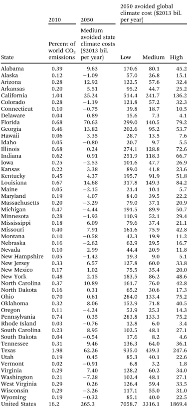
8.B. Global-warming damage costs eliminated by 100% WWS in each state
This section provides estimates of two kinds of climate change costs due to greenhouse gas (GHG) emissions from energy use (Table 8). GHG emissions are defined here to include emissions of carbon dioxide, other greenhouse gases, and air pollution particles that cause global warming, converted to equivalent carbon dioxide. A 100% WWS system in each state would eliminate such damages. The two kinds of costs calculated are
(1) The cost of climate change impacts to the world and U.S. attributable toemissions of GHGs from each of the 50 states, and (2) The cost of climate-change impactsborneby each state due to U.S. GHG emissions.
Costs due to climate change include coastal flood and real estate damage costs, energy-sector costs, health costs due to heat stress and heat stroke, influenza and malaria costs, famine costs, ocean acidification costs, increased drought and wildfire costs,
Table 6 ( continued ) State (a) 2013 average LCO E con ven-tion al fuels ( b per kWh) (b) 2050 av erage LCO E con ven-tion al fuels ( b per kWh) (c) 2050 average L COE of WWS ( b per kWh) (d) 2050 avera ge elec tricit y cos t sav-ing s per per son per yea r ($ per person per year) (e) 2050 avera ge air qualit y dam age sav-ings per per son per year due to WWS ($ per per son per yea r) (f) 2050 av erage cli-mate cost savin gs to state per per son per year du e to WWS ($ per per son per yea r) (g) 2050 avera ge cli-mat e cost savi ngs to world per per son per year due to WWS ($ per per son per year) (h) 2050 avera ge energ y + air qualit y dam age + world cli-ma te cost savi ngs du e to W WS ($ per per son per yea r) Virgini a 11.1 10.5 11.2 142 1255 676 5501 6898 Washi ngton 9.4 9.0 9.4 85 949 635 4195 5229 West Virgini a 10.6 10.4 9.2 703 1259 172 38911 40 873 Wiscon sin 10.1 11.3 10.6 318 1197 548 9264 10 779 Wyoming 9.9 9.9 8.3 1382 787 612 75 614 77 783 United State s 11.11 10.55 9.78 263 1491 661 8265 10 019 a (a) The 2013 LCO E cos t fo r conventi onal fue ls in each stat e com bines the esti mated d istribution of con ventional and WWS ge nerators in 2013 with 2013 me an L COEs fo r each generator from Table 5. Costs include all-di stanc e transmi ssion, pi pelines , and distribution, but they exclude ext ernalit ies. (b) Same as (a), but fo r a 2050 BAU ca se (ESI) and 2050 LCO Es for each ge nerator fro m Table 5. (c) The 2050 LCOE of WWS in the state com bines the 2050 distr ibution of WW S generator s from Table 3 w ith the 2050 mean LCOEs for each WW S generato r fr om Table 5. The LCOE accoun ts fo r all-di stanc e tran smission an d distribution and storage (footnotes to Tables 2 and 5). (d) The total cos t o f electric ity use in the elec tr icity sector in the BAU (the produc t o f elec tricity use an d the LCOE) less the tota l cost in the electric ity sec tor in the WWS scenari o and less the annu alized cost of the assum ed effici ency impr ovemen ts in the elect ricity sector in the WW S scenari o. Se e ESI and ref. 9, fo r details . (e ) Total cos t o f air pollution per year in the stat e from Tab le 7 divide d b y the 2050 pop ulation of the state. (f ) Total clima te cost per yea r in the state due to U.S. emissio ns (Table 8) divide d b y the 2050 popu lation of the state. (g) Total clima te cost per yea r to the w orld du e to stat e’s emissi ons (Tab le 8) d ivi ded by the 2050 pop ulation of the state. (h) The sum of colum ns (d), (e) , and (g).