Daniel Garcia-Macia
Stanford UniversityChang-Tai Hsieh
University of Chicago and NBERPeter J. Klenow
∗ Stanford University and NBERJune 30, 2015
Abstract
Entering and incumbent plants can create new products and displace existing products. Incumbents can also improve their existing products. How much of aggregate growth occurs through each of these channels? Using U.S. Census data on manufacturing plants from 1992, 1997 and 2002, we arrive at three main conclusions: First, most growth appeared to come from incumbent innovation rather than innovation by entrants. We infer this from the modest employment share of entering plants. Second, most growth seems to have occurred through improvements of existing varieties rather than creation of brand new varieties. We infer this because of modest net entry of plants and gently falling exit rates as plants expand, suggesting they produce better products more than a wider array of products. Third, own-product improvements by incumbents appear to have been more im-portant than creative destruction. We infer this because the distribution of job creation and destruction had thinner tails than implied by a model with a dominate role for creative destruction.
∗We thank Ufuk Akcigit and Andy Atkeson for very helpful comments. For financial support, Hsieh is grateful to Chicago’s Initiative for Global Markets (IGM) and Klenow to the Stanford Institute for Economic Policy Research (SIEPR). Any opinions and conclusions expressed herein are those of the authors and do not necessarily represent the views of the U.S. Census Bureau. All results have been reviewed by the U.S. Census Bureau to ensure no confidential information is disclosed.
1.
Introduction
Innovating firms can improve on existing products made by other firms, thereby gaining profits at the expense of those competitors. Such creative destruction plays a central role in many theories of growth. This goes back to at least Schum-peter (1939), carries through Stokey (1988), Grossman and Helpman (1991), and Aghion and Howitt (1992), and continues with more recent models such asKlette and Kortum(2004).Aghion et al.(2014) provide a recent survey.
Other growth theories emphasize the importance of firms improving their own products, rather than displacing other firms’ products. Krusell(1998) and
Lucas and Moll(2014) are examples. Some models combine creative destruc-tion and quality improvement by existing firms on their own products – see chapter 12 inAghion and Howitt(2009) and chapter 14 inAcemoglu(2011). A recent example isAkcigit and Kerr(2015), who also provide evidence that firms are more likely to cite their own patents and hence build on them.
Still other theories emphasize the contribution of brand new varieties to growth. Romer (1990) is the classic reference, andAcemoglu (2003) andJones
(2014) are some of the many follow-ups. Studies such as Howitt (1999) and
Young(1998) combine variety growth with quality growth.
Ideally, one could directly observe the extent to which new products sub-stitute for or improve upon existing products. Broda and Weinstein(2010) and
Hottman et al.(2014) are important efforts along these lines for consumer non-durable goods. Such high quality scanner data has not been available or ana-lyzed in the same way for consumer durables, producer intermediates, or pro-ducer capital goods – all of which figure prominently in theories of growth.1
We pursue a complementary approach. We try to infer the sources of growth indirectly from empirical patterns of firm and plant dynamics. The influential papers by Baily et al. (1992) and Foster et al. (2001) document the contribu-tions of entry, exit, reallocation, and within-plant productivity growth to over-1Gordon(2007) andGreenwood et al.(1997) emphasize the importance of growth embodied
all growth with minimal model assumptions. We consider a specific growth model with a limited set of parameters. Like us, Lentz and Mortensen (2008) andAcemoglu et al. (2013) conduct indirect inference on growth models with manufacturing data (from the U.S. and Denmark, respectively). They fully en-dogenize growth, whereas we consider exogenous growth models. The trade-off is that they focus on creative destruction, whereas we further incorporate new varieties and own-variety improvements by incumbents.
We use data on plants from U.S. manufacturing censuses in 1992, 1997 and 2002. Over this period, we calculate aggregate TFP growth, the exit rate of plants by age and employment, employment by age, job creation and destruction rates across plants, growth in the total number of plants, and moments of the em-ployment distribution across plants (the min, median, and mean). The param-eter values which best fit these moments lead to three conclusions. First, most growth appears to come from incumbents rather than entrants. This is because the employment share of entrants is modest. Second, most growth seems to occur through quality improvements rather than brand new varieties. Third, own-variety improvements by incumbents loom larger than creative destruc-tion (by entrants and incumbents).
The rest of the paper proceeds as follows. Section 2 lays out the parsimo-nious exogenous growth model we use. Section 3 briefly describes the U.S. manufacturing census data we exploit. Section 4 presents the model parameter values which best match the moments from the data. Section 5 concludes.
2.
An Exogenous Growth Model
We adapt theKlette and Kortum(2004) model of quality ladder growth through creative destruction. Firms produce multiple varieties and grow when they improve upon and capture the varieties produced by other firms. Entrants try to improve on existing varieties and take them over in the process. Incumbent firms die when their last varieties are captured by other firms (incumbents or
entrants). Unlike Klette-Kortum we treat the arrival rates of creative destruction from entrants and incumbents as exogenously fixed parameters, rather than being endogenously determined by underlying preferences, technology, and market structure. This allows us to keep the model parsimonious while adding exogenous arrival rates of new varieties from entrants, new varieties from in-cumbents, and own-variety quality innovations by incumbents.
Our set-up follows Klette-Kortum with these differences:
• Time is discrete (rather than continuous)
• There are a finite number of varieties (rather than a continuum)
• Innovation is exogenous (rather than endogenous)
• Demand for varieties is CES with elasticityσ ≥1(rather thanσ = 1)
• The number of varieties is growing (rather than fixed)
• Incumbents can improve the quality of their own varieties (rather than quality improvements only coming from other incumbents or entrants)
• Creative destruction by incumbents may be directed toward quality levels near the firm’s existing quality levels (rather than being undirected)
• Creative destruction by entrants may be directed toward lower quality lev-els (rather than being undirected)
Aggregate output
Total outputY in the economy is given by:
Yt =
"Mt X
j=1
(qj,tyj,t)
1−1/σ
whereM is the total number of varieties,qj is the quality of varietyj, andyj is
the quantity produced of varietyj. The production function for each variety is linear in laboryj =lj.
Static problem of the firm
Firms control multiple varieties, but we assume they are still monopolistic com-petitors for each variety. We assume further that there is an overhead cost of production that must be expended before choosing prices and output. This assumption allows the highest quality producer to charge the standard markup over marginal cost (the threat of limit pricing vs. the next lowest quality pre-vents the competitor from producing). Without this assumption, firms would engage in limit pricing and markups would be heterogeneous as inPeters(2013).
Assuming firms face the same wage, revenue generated by varietyjis
pjyj =
σ−1
σ
σ−1
PσY W1−σqjσ−1 ∝qjσ−1
whereP is the aggregate price level,Y is aggregate output, andW is the wage. Labor employed in producing varietyjis also proportional toqjσ−1:
lj =
σ−1
σ
σ
P W
σ
Y qjσ−1 ∝qjσ−1
Thus a firm’s revenue and employment are both proportional to the sum of power qualities qjσ−1 of the varieties operated by the firm.2 In the special case
ofσ = 1assumed by Klette-Kortum, all varieties have the same employment, and a firm’s employment is proportional to the number of varieties it controls. We will find it important to allowσ > 1, so that firms can be larger when they have higher quality products rather than just a wider array of products.
Aggregate productivity
Labor productivity in the economy is given by
Yt/L=M
1
σ−1
t
"Mt X
j=1 qσj,t−1
Mt
#σ−11.
whereLis total labor across all varieties (which is exogenously fixed in supply). The first term captures the benefit of having more varieties, and the second term is the power mean of quality across varieties.
Exogenous innovation
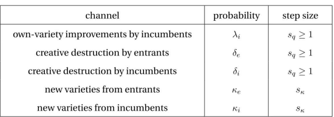
There is an exogenous arrival rate for each type of innovation. The notation for each type is given in Table1. The probabilities shown are per variety a firm produces. The probability of a firm improving any given variety it produces is
λi, and such improvement is associated with step sizesq ≥ 1. If a firm fails to
improve on a given variety it produces, then that variety is vulnerable to creative destruction by other (incumbent or entrant) firms. A fraction δi of vulnerable
varieties is creatively destroyed by another incumbent, and a fractionδe by an
entrant. Creative destruction also comes with step sizesq.
Table 1: Channels of Innovation
channel probability step size
own-variety improvements by incumbents λi sq≥1
creative destruction by entrants δe sq≥1
creative destruction by incumbents δi sq≥1
new varieties from entrants κe sκ
new varieties from incumbents κi sκ
incum-bents – again per existing variety produced by an incumbent. These arrivals are independent of other innovation types. The quality of each new variety is drawn at random from the current distribution of qualities, but a scaling factor sκ is
applied to each quality. The arrival rate of brand new varieties affects growth in the number of firms (tied toκeandκi), while the quality of new varieties (sκ)
affects the size of new firms.
On top of the seven parameters listed in Table1, we add three more param-eters. Klette-Kortum assumed creative destruction was undirected. We find that, when combined with σ > 1, undirected creative destruction leads to a thick-tailed distribution of employment growth rates. Firms can capture much better varieties than their own, growing rapidly in the process. Incumbents on the losing side of creative destruction can lose their best varieties, leaving them with low quality varieties and steeply negative growth. To allow some control over the distribution of tail growth rates in the model, we allow for the possibility that creative destruction is directed. We setρito be quality quantiles
in which incumbent creative destruction is directed. Ifρi = 0.1then incumbent
creative destruction occurs within quality deciles.3 If ρ
i = 1 then incumbent
creative destruction is undirected. For entrants, we assume creative destruction targets the lowest quality varieties, specifically the lowest varieties commanding
ρeshare of employment.4 The last parameter is the overhead cost of production,
which pins down the minimum firm size.
Note that each innovation is proportional to an existing quality level. Thus, if innovative effort was endogenous, there would be a positive knowledge exter-nality to research unless all research was done by firms on their own products. Such knowledge externalities are routinely assumed in the quality ladder litera-ture, such asGrossman and Helpman(1991),Kortum(1997),Klette and Kortum
(2004), andAcemoglu et al.(2013).
3As all arrival rates are per existing variety, the quantiles are defined for each individual
variety. We also allow brand new varieties created by incumbents to be directed in this way.
4Defining ρ
e as an employment share preserves an analytic expression for aggregate productivity growth.
Output growth
Total output grows at rate
1 +gY = [(1 +κe+κi) (1 +gq)]
1
σ−1
The κ components correspond to the creation of new varieties. The (1 +gq)
component reflects growth in average quality per variety. The growth rate of the power mean of quality levels across varieties is:
1 +gq =
sσ−1
κ (κe+κi) + 1 + sσq−1−1
(λi+ (1−λi) (ρeδe+δi))
1 +κe+κi
3.
U.S. Manufacturing Census Data
We use data from U.S. manufacturing Censuses to quantify dynamics of entry, exit, and survivor growth. We mostly use the 1992, 1997 and 2002 Censuses, stopping at 2002 because the NAICS definitions were changed from 2002 to 2007. We focus onplants rather than firms, because mergers and acquisitions can wreak havoc with our strategy to infer innovation from growth dynamics.
We are ultimately interested in decomposing the sources of TFP growth into contributions from different types of innovation. We therefore start by calcu-lating manufacturing-wide TFP growth. We take this from the U.S. Bureau of Labor Statistics Multifactor Productivity Growth. Converting their gross output measure to value added, TFP growth averages 3.0 percent per year from 1987– 2011 (the timespan of their data). The number of manufacturing plants in the U.S. Census of Manufacturing, meanwhile, rose 0.5 percent per year from 1972 to 2002.
Since the Census does not ask about a plant’s age directly, we infer it from the first year a plant shows up in the Census going back to 1963. We therefore have more complete data on the age of plants in more recent years. We use this data to calculate exit by age from 1992 to 1997. We then combine it with the
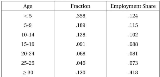
assumption of 0.5 percent per year growth in the number of entering plants to calculate the share of plants by age brackets of less than 5 years old, 5 to 9 years old, 10 to 14 years old, and so on until age 30 years and above. See the first column of Table2for the resulting density. About one-third of plants are less than 5 years old, and about one-eighth of plants are 30 years or older.
Table 2: Plants by Age
Age Fraction Employment Share
<5 .358 .124
5-9 .189 .115
10-14 .128 .102
15-19 .091 .088
20-24 .068 .081
25-29 .046 .073
≥30 .120 .418
Note: Author calculations from U.S. Census of Manufacturing plants in 1992 and 1997.
We report the share of employment by age in U.S. manufacturing in the second column of Table2. Young plants are much smaller on average, as their employment share (12 percent) is much lower than their fraction of plants (36 percent). Older surviving plants are much larger, comprising only 12 percent of plants but employing almost 42 percent of all workers in U.S. manufacturing. According to Hsieh and Klenow (2014), rapid growth of surviving plants is a robust phenomenon across years in the U.S. Census of Manufacturing.
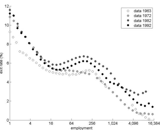
We plot how a plant’s exit rate varies with its size in Figure1. The exit rate is annualized based on successive years of the Census. The dots labeled “1992” are based on exit from 1992 to 1997, those labeled “1982” are based on exit from 1982 to 1987, and so on back to “1963”. As shown, the annual exit rate is about 10 percent for plants with a single employee, declines to about 6 percent for
Figure 1: Empirical Exit by Size in the U.S. Census of Manufacturing
plants with several hundred employees, then falls further to about 1 percent for plants with thousands of workers.
Figure 2, from Davis et al. (1998), plots the distribution of annual job cre-ation and destruction rates in U.S. manufacturing from 1973–1988. These rates are bounded between -2 (exit) and +2 (entry) because they are the change in employment divided by the average of last year’s employment and current year’s employment. The distribution on the vertical axis is the percent of all creation or destruction contributed by plants in each bin. We also target the absolute rates of job creation (11.1 percent) and job destruction (11.0 percent), and the absolute rates of job creation from entrants (3.0 percent) and job destruction from exiters (3.0 percent).
Figure 2: Job Creation and Destruction Rates in U.S. Manufacturing (via Davis, Haltiwanger and Schuh, 1998)
Lastly, we target several moments of the employment distribution across U.S. manufacturing plants: the minimum (1 employee), the mean (50 employ-ees), and the plant size of the median worker (900).
4.
Indirect Inference
We now compare moments from model simulations to the manufacturing mo-ments we calculated in the previous section. Our aim is to indirectly infer the sources of innovation. Our logic is that plant dynamics are a byproduct of inno-vation. Entrants reflect a combination of new varieties and creative destruction
of existing varieties. The better the new varieties, the bigger the employment share of entrants. When a plant expands, it does so because it has innovated on its own varieties, created new varieties, or captured varieties previously pro-duced by other incumbents. When a plant contracts it is because it has failed to improve its products or add products to keep up with aggregate growth (and hence real wage growth), or because it lost some of its varieties to creative de-struction from entrants or other incumbents. Outright exit occurs, as inKlette and Kortum(2004), when a plant loses all of its varieties to creative destruction. Because creative destruction is independent across a plant’s varieties (by assumption), plants with more varieties should have lower exit rates. Plants with higher qualities should be larger and potentially more protected against exit, as they have a lower likelihood of being captured by entrants who target the bottom of the quality distribution.
Simulation algorithm
Each firm’s static price and employment can be solved analytically, but we have to numerically compute the firm-level quality distribution. Compared to the
Klette and Kortum(2004) environment, our additional channels of innovation, as well as the elastic demand for quality (σ >1), preclude analytical results. Our simulation algorithm consists of the following steps:
1. Specify the distribution of quality across varieties.
2. Simulate life paths for entering plants such that the total number of plants observed, including incumbents, is the same as in U.S. from 1992–2002 (321,000 on average, including administrative record plants).
3. Each entrant has one initial variety, captured or newly created. In each year of its lifetime, it faces a probability of each type of innovation per variety it owns, as in Table 1. A firm’s life ends when it loses all of its varieties or when it reaches age 100.
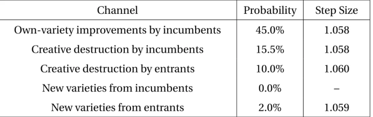
Table 3: Inferred Parameter Values
Channel Probability Step Size Own-variety improvements by incumbents 45.0% 1.058
Creative destruction by incumbents 15.5% 1.058 Creative destruction by entrants 10.0% 1.060
New varieties from incumbents 0.0% – New varieties from entrants 2.0% 1.059
4. Based on an entire population of simulated firms of all ages, compute the joint distribution of quality and variety across firms. Calculate moments of interest (e.g. exit by size).
5. Repeat steps 1 to 4 until all moments converge. In each iteration, update the guess for the distribution of qualities by combining elements from the previous iteration’s guess.
6. Repeat steps 1 to 5, searching for parameter values to minimize the abso-lute distance between the simulated and empirical moments.
Sources of growth
We present our inferred parameter values in Table 3. We will first discuss the inferred parameter values and the implications of these values for the sources of growth. We will then examine why the data fitting exercise yields the param-eters it does by shutting down each source of innovation.
We infer a 45 percent arrival rate for own-variety quality improvements by incumbents. Conditional on no own-innovation, quality improvements through creative destruction occur 15.5 percent of the time by other incumbents, and
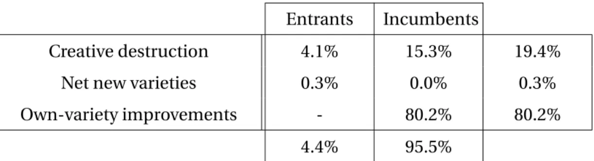
Table 4: Inferred Sources of Growth
Entrants Incumbents
Creative destruction 4.1% 15.3% 19.4% Net new varieties 0.3% 0.0% 0.3% Own-variety improvements - 80.2% 80.2%
4.4% 95.5%
10 percent of the time by entrants. The step size is 5.9 percent.5 Incumbent
creative destruction is estimated to be within deciles (ρi = 0.1), and entrant
cre-ative destruction is targeted toward lower-than-average quality quantiles (ρe =
0.41). The latter makes entrant quality smaller than average incumbent quality, and also contributes to a higher exit rate for smaller (lower quality on average) firms. New varieties arrive at a 2 percent annual rate, and come entirely from entrants. But overhead costs kill off varieties so that net growth in varieties matches the 0.5 percent per year growth in the number of plants.
Table4presents the implied sources of growth. About 19 percent of growth comes from creative destruction. Own-variety improvements by incumbents account for 80 percent. New varieties a la Romer (1990) are the remainder at less than 1 percent. Incumbents are the dominant source of growth (over 95 percent), with entrants contributing under 5 percent. Aghion et al. (2014) provide complementary evidence for the importance of incumbents based on their share of R&D spending.
At this point, a few key questions arise: What empirical moments suggest the presence of own-variety improvements? And how well does a model with only creative destruction fit the data? To help answer these questions, we examine a sequence of models as listed in Table 5. We start with the baseline Klette-5We could allow a different step size for own innovation than for creative destruction. When
Table 5: Simulated Models Klette-Kortum KK1 Klette-Kortum KK3 Directed Creative Destr. New Varieties Own Innov.
σ 1 3 3 3 3
Creative destruction √ √ √ √ √
Directed Creative Destr. √ √ √
New varieties √ √
Own-variety improvements √
Kortum model, which features σ = 1 and only creative destruction. Then we generalize the Klette-Kortum model toσ > 1, which allows high quality varieties to have employment attached. We next allow for directed creative destruction. Then we add the creation of brand new varieties by entrants and incumbents. Finally, we add own-variety improvements by incumbents.
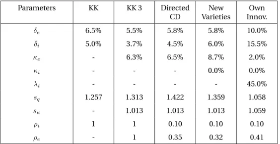
Table 6 reports the parameter values we infer for each model. By adding layers to the Klette-Kortum model, we progressively achieve a better fit with the data. The models from KK3 onwards have entry of new varieties to replace low-quality varieties exiting due to overhead costs. Only the models with last two models have positive net variety growth.
To provide some intuition, let us start with the baseline Klette-Kortum model. In this model, the average exit level, together with the exit by age slope, pin down the arrival rate of creative destruction by entrants and incumbents. In-tuitively, the exit rate of the smallest firm in the baseline Klette-Kortum model is simply the probability that the single variety owned by the smallest firm is improved upon by another firm. In this model, the exit rate of a one-variety firm is (δe+δi) (1−δi). I.e., the sum of the probability of creative destruction
by an entrant or an incumbent firm, times the probability that the firm does not creatively destroy a variety from another incumbent. Around 11.5% of the
Table 6: Parameter Values in the Simulated Models
Parameters KK KK 3 Directed
CD
New Varieties
Own Innov.
δe 6.5% 5.5% 5.8% 5.8% 10.0%
δi 5.0% 3.7% 4.5% 6.0% 15.5%
κe - 6.3% 6.5% 8.7% 2.0%
κi - - - 0.0% 0.0%
λi - - - - 45.0%
sq 1.257 1.313 1.422 1.359 1.058
sκ - 1.013 1.013 1.013 1.059
ρi 1 1 0.10 0.10 0.10
ρe - 1 0.35 0.32 0.41
varieties are subject to creative destruction each year. A large step size (26%) is therefore needed to match the annual growth rate of 3%. This pattern holds for all of the models save the one with own-variety quality improvements.
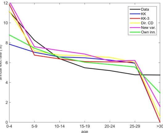
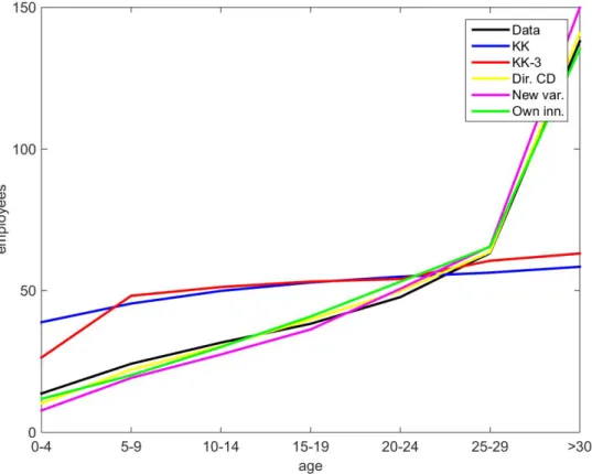
Figure 3 plots the exit rate of plants by age in each model vs. that in the data. The fit is similar for all models. Figure4plots the size (average number of employees) of plants by age. Only models with new varieties are able to replicate the amount of growth in size by age seen in the data. As shown in Table 6, entrants target the lower third or so of the quality distribution. This makes quality grow with age, helping to fit the size growth with age in the data.
Figures5through9contrast the exit rate by size in each model with the data counterpart. In the original Klette-Kortum model withσ = 1 (KK), firm size is proportional to its number of varieties. Firms with many varieties are unlikely to lose them all at once, as creative destruction is independent across varieties. Thus exit falls too sharply with size, as displayed in Figure5. This failure of the original Klette-Kortum model leads us to considerσ >1, so that higher quality varieties employ more workers in their production. As a result, big firms tend to
Figure 5: Model Fit, Exit by Size, Klette-Kortum
have higher quality varieties rather than just more varieties.6 A higher elasticity
of substitution (σ = 3in KK 3) flattens out the exit rate by size, as shown in Figure 6. When we allow for directed creative destruction, which is helpful to better fit size by age, the exit rate falls more with size (Figure 7). Adding new varieties to match growth in the number of plants has little effect (Figure 8). The fit with incumbents improving their varieties (Figure7) is best of all.
Figures10through14plot job creation and destruction for each model com-pared to the data. These Figures display theshareof job creation and destruc-tion due to firsm exiting, contracting by various amounts, expanding by various 6In the KK 3 model, overhead costs are crucial for obtaining a stationary quality (and
therefore size) distribution. The overhead costs kill off lower quality varieties, offsetting the spreading impact of random arrival of quality innovations.
amounts, and entering. All of the models come close to fitting the overall job creation and destruction rates of around 11 percent each.
As mentioned earlier, models with undirected innovation generate unrealis-tically thick tails of job creation and destruction. This is most striking in Figure
11for the Klette-Kortum model withσ= 3. When firms can acquire much better varieties they routinely grow by a lot; when they can lose their best varieties and retain their worst ones they can shrink by a lot.
Models with directed innovation do much better at matching the empirical distribution of job creation and destruction. This can be seen in Figures12to
14. When incumbents target their own quality decile for creative destruction, the varieties they acquire and lose are similar to the varieties they start with and retain, making job creation and destruction less extreme.
Adding own-variety improvements fits the job creation and destruction pic-ture best of all. With frequent own-variety improvements, the step size can be much smaller – 6% rather than 26–42% in Table6. Thus firms can experience many modest increases in their size, and fewer extreme increases or decreases. See Figure14.
5.
Conclusion
How much of innovation takes the form of creative destruction versus firms improving their own products versus new varieties? How much of innovation occurs through entrants vs. incumbents? We try to infer the sources of in-novation by matching manufacturing plant dynamics in the U.S. We conclude that creative destruction is vital for understanding job destruction and exit and accounts for something like 20 percent of growth. Own-product quality im-provements by incumbents appear to be the source of 80 percent of growth. Variety growth contributes little, as creation of new varieties is offset by exit of low quality varieties.
we identify may have implications for business stealing effects vs. knowledge spillovers, and hence the social vs. private return to innovation. The impor-tance of creative destruction ties into political economy theories in which in-cumbents block entry and hinder growth and development, such as Krusell and Rios-Rull(1996),Parente and Prescott(2002), andAcemoglu and Robinson
(2012).
It would be interesting to extend our analysis to other sectors, time periods, and countries. Retail trade experienced a big-box revolution in the U.S. led by Wal-Mart’s expansion. Online retailing has made inroads at the expense of brick-and-mortar stores. Chinese manufacturing has seen entry and expan-sion of private enterprises at the expense of state-owned enterprises (Hsieh and Klenow(2009)). In India, manufacturing incumbents may be less important for growth given that surviving incumbents do not expand anywhere near as much in India as in the U.S. (Hsieh and Klenow(2014)).
Our conclusions are tentative in part because they are model-dependent. We followed the literature in several ways that might not be innocuous for our inference:
We assumed that spillovers are just as strong for incumbent innovation as for entrant innovation. Young firms might instead generate more knowledge spillovers than old firms do –Akcigit and Kerr(2015) provide evidence for this hypothesis in terms of patent citations by other firms.
We assumed no frictions in employment growth or misallocation of labor across firms. In reality, the market share of young plants could be suppressed by adjustment costs, financing frictions, and uncertainty. In addition to ad-justment costs for capital and labor, it may take plants awhile to build up a cus-tomer base, as in work byFoster et al.(2013) andGourio and Rudanko(2014). Ir-reversibilities could combine with uncertainty about the plant’s quality to keep young plants small, as in Jovanovic(1982) model. Markups could vary across varieties and firms. All of these would create a more complicated mapping from plant employment growth to plant innovation.
Figure 10: Model Fit, Job Creation and Destruction, Klette-Kortum
References
Acemoglu, Daron, “Labor- and Capital-Augmenting Technical Change,”Journal of the European Economic Association, 2003,1(1), 1–37.
,Introduction to Modern Economic Growth, Princeton University Press, 2011.
and James Robinson, Why Nations Fail: Origins of Power, Poverty and Prosperity, Crown Publishers (Random House), 2012.
, Ufuk Akcigit, Nicholas Bloom, and William R Kerr, “Innovation, Reallocation and Growth,” Working Paper 18993, National Bureau of Economic Research 2013.
Figure 12: Model Fit, Job Creation and Destruction, Directed Creative Destruction
Aghion, Philippe and Peter Howitt, “A Model of Growth Through Creative Destruction,”
Econometrica, 1992,60(2), pp. 323–351.
and , The Economics of Growth, Massachusetts Institute of Technology (MIT) Press, 2009.
, Ufuk Akcigit, and Peter Howitt, “What Do We Learn From Schumpeterian Growth Theory?,”Handbook of Economic Growth, 2014,2B, 515–563.
Akcigit, Ufuk and William R. Kerr, “Growth through Heterogeneous Innovations,” 2015.
Baily, Martin Neil, Charles Hulten, and David Campbell, “Productivity Dynamics in Manufacturing Plants,”Brookings Papers: Microeconomics, 1992,4, 187–267.
Broda, Christian and David E Weinstein, “Product Creation and Destruction: Evidence and Implications,”American Economic Review, 2010,100(3), 691–723.
Davis, Steven J, John C Haltiwanger, and Scott Schuh, “Job creation and destruction,”
MIT Press Books, 1998.
Foster, Lucia, John C Haltiwanger, and C.J. Krizan, “Aggregate productivity growth. Lessons from microeconomic evidence,”New developments in productivity analysis, 2001, pp. 303–372.
, John Haltiwanger, and Chad Syverson, “The Slow Growth of New Plants: Learning about Demand?,” 2013.
Gordon, Robert J,The measurement of durable goods prices, University of Chicago Press, 2007.
Gourio, Francois and Leena Rudanko, “Customer capital,”Review of Economic Studies, forthcoming, 2014.
Greenwood, Jeremy, Zvi Hercowitz, and Per Krusell, “Long-run implications of investment-specific technological change,”American Economic Review, 1997,87(3), 342–362.
Grossman, Gene M and Elhanan Helpman, “Quality ladders in the theory of growth,”
Review of Economic Studies, 1991,58(1), 43–61.
Hottman, Colin, Stephen J Redding, and David E Weinstein, “What is’ Firm Heterogeneity’in Trade Models? The Role of Quality, Scope, Markups, and Cost,” Technical Report, National Bureau of Economic Research 2014.
Howitt, Peter, “Steady Endogenous Growth with Population and R & D Inputs Growing,”
Journal of Political Economy, 1999,107(4), pp. 715–730.
Hsieh, Chang-Tai and Peter J Klenow, “Misallocation and manufacturing TFP in China and India,”Quarterly Journal of Economics, 2009,124(4), 1403–1448.
and Peter J. Klenow, “The Life Cycle of Plants in India and Mexico,”Quarterly Journal of Economics, forthcoming, 2014.
Jones, Charles I., “Life and Growth,”Journal of Political Economy, forthcoming, 2014.
Jovanovic, Boyan, “Selection and the Evolution of Industry,”Econometrica, 1982,50(3), 649–670.
Klette, Tor Jakob and Samuel Kortum, “Innovating firms and aggregate innovation,”
Journal of Political Economy, 2004,112(5), 986–1018.
Kortum, Samuel S., “Research, Patenting, and Technological Change,” Econometrica, 1997,65(6), 1389–1419.
Krusell, Per, “How is R&D Distributed Across Firms? A Theoretical Analysis,” 1998.
and Jose-Victor Rios-Rull, “Vested interests in a positive theory of stagnation and growth,”Review of Economic Studies, 1996,63(2), 301–329.
Lentz, Rasmus and Dale T Mortensen, “An empirical model of growth through product innovation,”Econometrica, 2008,76(6), 1317–1373.
Lucas, Robert E Jr. and Benjamin Moll, “Knowledge Growth and the Allocation of Time,”
Journal of Political Economy, 2014,122(1).
Peters, Michael, “Heterogeneous Mark-ups, Growth and Endogenous Misallocation,” 2013.
Romer, Paul M., “Endogenous Technological Change,” Journal of Political Economy, 1990,98(5), pp. S71–S102.
Schumpeter, Joseph A.,Business cycles, Cambridge University Press, 1939.
Stokey, Nancy L, “Learning by doing and the introduction of new goods,” Journal of Political Economy, 1988,96(4), 701–717.
Young, Alwyn, “Growth without Scale Effects,”Journal of Political Economy, 1998,106