An Empirical Study
Kai-Bo Duan1 and S. Sathiya Keerthi21 BioInformatics Research Centre, Nanyang Technological University, Nanyang Avenue, Singapore 639798
[email protected] 2 Yahoo! Research Labs,
210 S. DeLacey Street, Pasadena, CA-91105, USA [email protected]
Abstract. Multiclass SVMs are usually implemented by combining sev-eral two-class SVMs. The one-versus-all method using winner-takes-all strategy and the one-versus-one method implemented by max-wins vot-ing are popularly used for this purpose. In this paper we give empirical evidence to show that these methods are inferior to another one-versus-one method: one-versus-one that uses Platt’s posterior probabilities together with the pairwise coupling idea of Hastie and Tibshirani. The evidence is par-ticularly strong when the training dataset is sparse.
1
Introduction
Binary (two-class) classification using support vector machines (SVMs) is a very well developed technique [1] [11]. Due to various complexities, a direct solu-tion of multiclass problems using a single SVM formulasolu-tion is usually avoided. The better approach is to use a combination of several binary SVM classi-fiers to solve a given multiclass problem. Popular methods for doing this are: all method using winner-takes-all strategy (WTA SVM); one-versus-one method implemented by max-wins voting (MWV SVM); DAGSVM [8]; and error-correcting codes [2].
Hastie and Tibshirani [4] proposed a good general strategy called pairwise couplingfor combining posterior probabilities provided by individual binary clas-sifiers in order to do multiclass classification. Since SVMs do not naturally give out posterior probabilities, they suggested a particular way of generating these probabilities from the binary SVM outputs and then used these probabilities together with pairwise coupling to do muticlass classification. Hastie and Tib-shirani did a quick empirical evaluation of this method against MWV SVM and found that the two methods give comparable generalization performances.
Platt [7] criticized Hastie and Tibshirani’s method of generating posterior class probabilities for a binary SVM, and suggested the use of a properly designed sigmoid applied to the SVM output to form these probabilities. However, the
N.C. Oza et al. (Eds.): MCS 2005, LNCS 3541, pp. 278–285, 2005. c
use of Platt’s probabilities in combination with Hastie and Tibshirani’s idea of pairwise coupling has not been carefully investigated thus far in the literature. The main aim of this paper is to fill this gap. We did an empirical study and were surprised to find that this method (we call it as PWC PSVM) shows a clearly superior generalization performance over MWV SVM and WTA SVM; the superiority is particularly striking when the training dataset is sparse.
We also considered the use of binary kernel logistic regression classifiers1
to-gether with pairwise coupling. We found that even this method is somewhat inferior to PWC PSVM, which clearly indicates the goodness of Platt’s prob-abilities for SVMs. The results of this paper indicate that PWC PSVM is the best single kernel discriminant method for solving multiclass problems.
The paper is organized as follows. In section 2, we briefly review the various implementations of one-versus-all and one-versus-one methods that are stud-ied in this paper. In section 3, we describe the numerical experiments used to study the performances of these implementations. The results are analyzed and conclusions are made in section 4. The manuscript of this paper was prepared previously as a technical report [3].
2
Description of Multiclass Methods
In this section, we briefly review the implementations of the multiclass methods that will be studied in this paper. For a given multiclass problem,M will denote the number of classes andωi, i= 1, . . . , Mwill denote theM classes. For binary classification we will refer to the two classes as positive and negative; a binary classifier will be assumed to produce an output function that gives relatively large values for examples from the positive class and relatively small values for examples belonging to the negative class.
2.1 WTA SVM
WTA SVM constructs M binary classifiers. The ith classifier output function ρi is trained taking the examples fromωias positive and the examples from all
other classes as negative. For a new examplex, WTA SVM strategy assigns it to the class with the largest value ofρi.
2.2 MWV SVM
This method constructs one binary classifier for every pair of distinct classes and so, all togetherM(M−1)/2 binary classifiers are constructed. The binary classifierCij is trained taking the examples fromωias positive and the examples fromωj as negative. For a new examplex, if classifierCij saysxis in classωi, then the vote for class ωi is added by one. Otherwise, the vote for class ωj is increased by one. After each of theM(M−1)/2 binary classifiers makes its vote, MWV strategy assignsxto the class with the largest number of votes.
2.3 Pairwise Coupling
If the output of each binary classifier can be interpreted as the posterior proba-bility of the positive class, Hastie and Tibshirani [4] suggested apairwise coupling
strategy for combining the probabilistic outputs of all the one-versus-one binary classifiers to obtain estimates of the posterior probabilities pi = Prob(ωi|x), i= 1, . . . , M. After these are estimated, the PWC strategy assigns the example under consideration to the class with the largestpi.
The actual problem formulation and procedure for doing this are as follows. Let Cij be as in section 2.2. Let us denote the probabilistic output of Cij as rij = Prob(ωi|ωi orωj). To estimate thepi’s, M(M −1)/2 auxiliary variables
µij’s which relate to the pi’s are introduced: µij =pi/(pi+pj). pi’s are then
determined so thatµij’s are close torij’s in some sense. The Kullback-Leibler distance betweenrij andµij is chosen as the measurement of closeness:
l(p) =
i<j
nij
rijlogµrij
ij + (1−rij) log
1−rij 1−µij
(1)
wherenijis the number of examples inωi∪ωjin the training set.2The associated score equations are (see [4] for details):
j=i
nijµij =
j=i
nijrij, i= 1,· · ·, M, subject to M
k=1
pk= 1 (2)
Thepi’s are computed using the following iterative procedure: 1. Start from an initial guess ofpi’s and correspondingµij’s 2. Repeat (i= 1, . . . , M, 1, . . .) until convergence:
– pi←pi·
j=inijrij
j=inijµij – renormalize the pi’s – recomputeµij’s
Let ˜pi = 2jrij/k(k−1). Hastie and Tibshirani [4] showed that the multi-category classification based on ˜pi’s is identical to that based on thepi’s obtained from pairwise coupling. However, ˜pi’s are inferior to the pi’s as estimates of posteriori probabilities. Also, log-likelihood values play an important role in the tuning of hyperparameters (see section 3). So, it is always better to use thepi’s as estimates of posteriori probabilities.
A recent paper [12] proposed two new pairwise coupling schemes for estima-tion of class probabilities. They are good alternatives for the pairwise coupling method of Hastie and Tibshirani.
2 It is noted in [4] that, the weightsn
ijin (1) can improve the efficiency of the estimates a little, but do not have much effect unless the class sizes are very different. In practice, for simplicity, equal weights (nij= 1) can be assumed.
Kernel logistic regression (KLR) [10] has a direct probabilistic interpretation built into its model and its output is the positive class posterior probability. Thus KLR can be directly used as the binary classification method in the PWC implementation. We will refer to this multiclass method as PWC KLR.
The output of an SVM, however, is not a probabilistic value, but an un-calibrated distance measurement of an example to the separating hyperplane in the feature space. Platt [7] proposed a method to map the output of an SVM into the positive class posterior probability by applying a sigmoid function to the SVM output:
Prob(ω1|x) =
1
1 +eAf+B (3)
wheref is the output of the SVM associated with examplex. The parameters A and B can be determined by minimizing the negative log-likelihood (NLL) function of the validation data. A pseudo-code for determiningAandB is also given in [7]; see [6] for an improved pseudo-code. To distinguish from the usual SVM, we refer to the combination of SVM together with the sigmoid function mentioned above as PSVM. The multiclass method that uses Platt’s probabilities together with PWC strategy will be referred to as PWC PSVM.
3
Numerical Experiments
In this section, we numerically study the performance of the four methods dis-cussed in the previous section, namely, WTA SVM, MWV SVM, PWC PSVM and PWC KLR. For all these kernel-based classification methods, the Gaussian kernel,K(xi,xj) =e−xi−xj2/2σ2
is employed. Each binary classifier, whether it is SVM, PSVM or KLR, requires the selection of two hyperparameters: a regular-ization parameterCand a kernel parameterσ2. Every multi-category
classifica-tion method included in our study involves several binary classifiers. In line with the suggestion made by Hsu and Lin [5], we take theC andσ2of all the binary
classifiers within a multiclass method to be the same.3The two hyperparameters
are tuned using 5-fold cross-validation estimation of the multiclass generaliza-tion performance. We select the optimal hyperparameter pair by a two-step grid search. First we do a coarse grid search using the following sets of values:C∈ {1.0e-3, · · ·, 1.0e+3} and σ2 ∈ {1.0e-3, · · ·, 1.0e+3}. Thus 49 combinations of C and σ2 are tried in this step. An optimal pair (Co, σ2o) is selected from this coarse grid search. In the second step, a fine grid search is conducted around (Co, σ2o), withC∈ {0.2Co,0.4Co,0.6Co,0.8Co, Co,2Co,4Co,6Co,8Co}andσ2∈ {0.2σ2
o,0.4σo2,0.6σ2o,0.8σo2, σ2o,2σ2o,4σo2,6σo2,8σo2}. All together, 81 combinations
of C and σ2 are tried in this step. The final optimal hyperparameter pair
is selected from this fine search. In each grid search, especially in the fine search step, it is quite often the case that there are several pairs of hyperpa-rameters that give the same cross validational classification accuracy. In such 3 An alternative is to choose theC and σ2 of each binary classifier to minimize the
Table 1.Basic information and training set sizes of the five datasets Dataset #Classes #Total Examples Training Set Sizes
Small Medium Large
ABE 3 2,323 280 560 1,120
DNA 3 3,186 300 500 1,000
SAT 6 6,435 1,000 1,500 2,000
SEG 7 2,310 250 500 1,000
WAV 3 5,000 150 300 600
a situation, we have found it worthwhile to follow some heuristic principles to select one pair of C and σ2 from these short-listed combinations. For the
methods with posteriori probability estimates, where a cross-validation esti-mate of error rate (cvErr) as well as a cross-validation estiesti-mate of negative log-likelihood (cvNLL) are available, the following strategies are applied se-quentially until we find one unique parameter pair: (a) select the pair with smallest cvErr value; (b) select the pair with smallest cvNLL value; (c) se-lect the pair with larger σ2 value; (d) select the pair with smaller C value; (e) select the pair with smallest 8-neighbor average cvErr value; (f) select the pair with smallest C value. Usually step (b) yields a unique pair of hyperpa-rameters. For the methods without posteriori probability estimates, step (b) is omitted.
The performance of the four methods are evaluated on the following datasets taken from the UCI collection: ABE, DNA,Satellite Image(SAT),Image Segen-tation (SEG) andWaveform (WAV). ABE is a dataset that we extracted from the dataset Letter by using only the classes corresponding to the characters “A”, “B” and “E”. Each continuous input variable of these datasets is nor-malized to have zero mean and unit standard deviation. For each dataset, we divide the whole data into a training set and a test set. When the training set size is large enough, all the methods perform equally very well. Differences be-tween various methods can be clearly seen only when the training datasets are sparse. So, instead of using a single training set size (that is usually chosen to be reasonably large in most empirical studies), we use three different training set sizes: small, medium and large. For each dataset, the basic information to-gether with the values of the three training set sizes are summarized in Table 1. For each dataset, at each training set size, the whole data is randomly parti-tioned into a training set and a test set 20 times by stratified sampling. For each such partition, after each multi-category classifier is designed using solely the training set, it is tested on the test set. The mean and standard devia-tion of the test set error rate (in percentage) are computed over the 20 runs. The results are reported in Table 2. Full details of all runs can be found at:
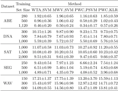
Table 2.Mean and standard deviation of test set error (in percentage) over 20 divisions of training and test sets, for the five datasets, at the three training set sizes (small, medium and large)
DatasetTraining Method
Set Size WTA SVM MWV SVM PWC PSVM PWC KLR ABE
280 1.92±0.65 1.96±0.65 1.16±0.63 1.85±0.59 560 0.96±0.36 1.06±0.42 0.58±0.29 1.02±0.43 1,120 0.46±0.20 0.50±0.24 0.34±0.17 0.57±0.26 DNA
300 10.15±1.26 9.87±0.90 9.23±1.73 9.73±0.75 500 7.84±0.79 7.67±0.93 7.41±1.14 7.80±0.71 1,000 5.59±0.39 5.72±0.57 5.50±0.69 5.76±0.54 SAT
1,000 11.07±0.58 11.03±0.73 10.27±0.92 11.20±0.55 1,500 10.08±0.49 10.20±0.51 10.05±0.60 10.23±0.42 2,000 9.51±0.31 9.61±0.39 9.47±0.65 9.66±0.37 SEG
250 9.43±0.54 7.97±1.23 6.66±2.24 7.54±1.24 500 6.51±0.99 5.40±1.04 5.19±0.74 4.83±0.68 1,000 4.89±0.71 4.35±0.79 4.08±0.52 3.96±0.68 WAV
150 17.21±1.37 17.75±1.39 13.20±3.70 15.59±1.13 300 15.43±0.97 15.96±0.98 12.97±2.02 14.71±0.72 600 14.09±0.55 14.56±0.80 13.47±1.09 13.81±0.41
4
Results and Conclusions
Let us now analyze the results from our numerical study. From Table 2 we can see that, PWC PSVM gives the best classification results and has significantly smaller mean values of test error. For WTA SVM, MWV SVM and PWC KLR, it is hard to tell which one is better.
To give a more vivid presentation of the results from the numerical study, we draw, for each dataset and each training set size, a boxplot to show the 20 test errors of each method, obtained from the 20 partitions of training and test. The boxplots are shown in Figure 1. These boxplots clearly support the observation that PWC PSVM is better than the other three methods. On some datasets, although the variances of PWC PSVM error rates are larger than those of other methods, the corresponding median values of PWC PSVM are much smaller than other three methods.
The boxplots also show that, as the training set size gets larger, the classi-fication performances of all four methods get better and the performance dif-ferences between them become smaller. This re-emphasizes the need for using a range of training set sizes when comparing two methods. A good method should work well, even at small training set size. PWC PSVM has this property.
We have also done a finer comparison of the methods by pairwiset-test. The results further consolidate the conclusions drawn from Table 2 and Figure 1. To
280 560 1120 0 0.5 1 1.5 2 2.5 3 3.5 4
Training Set Size
Test Error Rate( % )
−−−−−−−−−−−− Dataset: ABE −−−−−−−−−−−−
300 500 1000
4 5 6 7 8 9 10 11 12 13
Training Set Size
Test Error Rate( % )
−−−−−−−−−−−− Dataset: DNA −−−−−−−−−−−−
1000 1500 2000 8 9 10 11 12 13 14
Training Set Size
Test Error Rate( % )
−−−−−−−−−−−− Dataset: SAT −−−−−−−−−−−−
250 500 1000
2 3 4 5 6 7 8 9 10 11 12
Training Set Size
Test Error Rate( % )
−−−−−−−−−−−− Dataset: SEG −−−−−−−−−−−−
150 300 600
8 10 12 14 16 18 20 22
Training Set Size
Test Error Rate( % )
−−−−−−−−−−−− Dataset: WAV −−−−−−−−−−−−
For each dataset, at each training set size, from left to right, the four methods are: WTA_SVM, MWV_SVM, PWC_PSVM and PWC_KLR. Note:
Fig. 1.The boxplots of the four methods for the five datasets, at the three training set sizes (small, medium and large). For easy comparison the boxplots of the four methods are put side by side
keep the paper short, we are not including the description of the pairwiset-test
comparison and the p-values from the study. Interested readers may refer to our technical report [3] for details.
To conclude, we can say the following.WTA SVM,MWV SVMandPWC KLR are competitive with each other and there is no clear superiority of one method over another. PWC PSVM consistently outperforms the other three methods. The fact that the method is better than PWC KLR indicates the goodness of Platt’s posterior probabilities. PWC PSVM using one of the pairwise coupling schemes in [4] and [12] is highly recommended as the best kernel discriminant method for solving multiclass problems.
References
1. Boser, B., Guyon, I., Vapnik, V.: An training algorithm for optimal margin classi-fiers. In:Fifth Annual Workshop on Computational Learning Theory, Pittsburgh, ACM (1992) 144–152
2. Dietterich, T., Bakiri, G.: Solving multiclass problem via error-correcting output code.Journal of Artificial Intelligence Research, Vol. 2 (1995) 263–286
3. Duan, K.-B., Keerthi, S.S.: Which is the best multiclass SVM method? An empiri-cal study. Techniempiri-cal Report CD-03-12, Control Division, Department of Mechaniempiri-cal Engineering, National University of Singapore. (2003)
4. Hastie, T., Tibshirani, R.: Classification by pairwise coupling. In: Jordan, M.I., Kearns, M.J., Solla, A.S. (eds.):Advances in Neural Information Processing Sys-tems 10. MIT Press (1998)
5. Hsu, C.-W., Lin, C.-J.: A comparison of methods for multi-class support vector machines.IEEE Transactions on Neural Networks, Vol. 13 (2002) 415–425 6. Lin, H.-T., Lin, C.-J., Weng, R.C.: A note on Platt’s
proba-bilistic outputs for support vector machines (2003). Available:
http://www.csie.ntu.edu.tw/˜cjlin/papers/plattprob.ps
7. Platt, J.: Probabilistic outputs for support vector machines and comparison to regularized likelihood methods. In: Smola, A.J., Bartlett, P., Sch¨olkopf, B., Schu-urmans, D. (eds.):Advances in Large Margin Classifiers. MIT Press (1999) 61–74 8. Platt, J., Cristanini, N., Shawe-Taylor, J.: Large margin DAGs for multiclass classi-fication.Advances in Neural Information Processing Systems 12. MIT Press (2000) 543–557
9. Rifkin, R., Klautau, A.: In defence of one-versus-all classificaiton. Journal of Ma-chine Learning Research, Vol. 5 (2004) 101–141
10. Roth, V.: Probabilistic discriminant kernel classifiers for multi-class problems. In: Radig, B., Florczyk, S. (eds.):Pattern Recognition-DAGM’01. Springer (2001) 246– 253
11. Vapnik, V.:Statistical Learning Theory. Wiley Interscience (1998)
12. Wu, T.-F., Lin, C.-J., Weng, R.C.: Probability estimates for multi-class classifica-tion by pairwise coupling.Journal of Machine Learning Research, Vol. 5 (2004) 975–1005