The Distributed Parallel Machine and Assembly Scheduling Problem
with eligibility constraints
Sara Hatamia,i, Rubén Ruizb and Carlos Andrés-Romanoa,ii
a Departamento de Organización de Empresas, Universitat Politècnica de València.
Camino de Vera s/n, 46021, València, Spain.
a,ii [email protected]
b Grupo de Sistemas de Optimización Aplicada, Instituto Tecnológico de Informática, Ciudad Politécnica de la
Innovación, Edifico 8G, Acc. B. Universitat Politècnica de València, Camino de Vera s/n, 46021, València, Spain.
Abstract: In this paper we jointly consider several realistic scheduling extensions: First we study the distributed unrelated parallel machines problem where there is a set of identical factories with parallel machines in the production stage. Jobs have to be assigned to factories and to machines. Additionally, there is an assembly stage with a single assembly machine. Finished jobs at the manufacturing stage are assembled into final products in this second assembly stage. These two joint features are referred to as the Distributed Parallel Machine and Assembly Scheduling Problem or DPMASP. The objective is to minimize the makespan in the assembly stage. Due to technological constraints, machines cannot be idle and some jobs can be processed only in certain factories. We propose a mathematical model and two high-performing heuristics. The model is tested with two state-of-the-art solvers and, together with the heuristics, 2220 instances are solved in a comprehensive computational experience. Results show that the proposed model is able to solve moderately-sized instances, and that one of the heuristics is fast, giving optimal solutions close to optimum in less than half a second in the worst case.
Key words: Distributed Parallel Machines, Assembly Stage, Heuristics, Model.
1. Introduction
Nowadays, the manufacturing industry faces many challenges, namely globalization, increasing product variety, complexity and customer demands, shorter product life cycles, higher demand of customized goods instead of mass production, uncertain and dynamic global market, etc. Of course, the strong competition from emerging and established economies has to be considered as well. One of the many tools to face these challenges and to meet customer’s demands is to increase the product variety that companies offer. A wide product portfolio and diversified offer is a key asset to stay competitive in such an unpredictable and ever evolving market. Product variety has been defined by many authors as a number or collection of different things of a
particular class of the same general kind (Elmaraghy et al., 2013). In recent years, assembly systems are such as techniques that are mostly used mass production. They have been also employed in various manufacturing systems so as to increase flexibility and the capability to increase product variety. These types of manufacturing settings are referred to as Assembly Scheduling Problems (ASP).
In an assembly system, different operations are performed independently, and potentially in parallel, to produce different components which are later assembled into finished products in assembly lines. A high variety of finished products, made from different combinations of produced components, can be produced in assembly systems.
Manufacturing Systems (DMS). In a DMS environment, several independent production centers or factories are run in parallel at potentially different geographical places. Furthermore, distributed manufacturing allows for greater flexibility and resiliency (Sluga et al., 1998). Other benefits of DMS are: higher product quality, lower production costs, reduced risks (Kahn et al., 2004; Chan et al., 2005; Mahdavi et al., 2008). However, scheduling in DMS is more complicated than in a single production factory. In single production centers a job schedule for each set of machines has to be defined, while in DMSs, there are two interrelated decisions to be made: factory selection for each job and then scheduling at each factory.
As a conclusion, and in order to reap the benefits of both assembly systems (ASP) and distributed manufacturing (DMS), both aspects must be jointly considered.
In this paper we consider two manufacturing stages: production and assembly. For production we have a set of distributed factories and for assembly there is a single assembly facility. Each one of the f distributed production centers (factories) has unrelated parallel machines as a shop configuration whereas the assembly stage consists of a single machine. Transportation time for transferring jobs from production centers to assembly stage is assumed negligible. By considering the above model we define the studied problem in this paper as the Distributed Parallel Machine and Assembly Scheduling Problem (DPMASP).
More in specifically, in the DPMASP there is a set N of n jobs that has to be processed on a set F of f identical factories. Note that all factories are identical and have the same number of machines. Each factory has a set M of m unrelated parallel machines. Each job has to be processed at exactly one machine at one factory. Furthermore, there are eligibility constraints. LFj⊆F is the subset of factories where job j can be assigned, where f ≥|LFj|≥ 1, j=1…n job j can only be assigned to an eligible factory. There is a set T of t independent products. Each product is assembled at the single assembly machine MA. For the assembly of product h, h=1…t a subset Nh⊆N of jobs must have been produced at the distributed factories beforehand. Each job can only belong to an assembly program of a product, i.e.,
/
ht=1 Nh =n. The assembly of product h can only start when all jobs in Nh have been completed at the distributed factories. For the processing at the distributed manufacturing stage, pjk denotes the processing time of job j at machine k of any factory. Note that all factories are identical andhave the same number of machines. For the assembly stage, ph denotes the assembly time of product h. All processing times are positive, deterministic and known integer quantities. The objective in the proposed DPMASP is to assign jobs to machines at factories in the distributed manufacturing stage, to schedule all assigned jobs to each machine at each factory and to schedule products at the single machine assembly stage while minimizing the makespan at this assembly stage. As regards the computational complexity of the DPMASP we can conclude that it is an NP-Hard problem if n≫f since the regular parallel machines problem (even in the case where there are two identical machines, i.e., the P2//Cmax problem) is already NP-Hard according to the results of Lenstra et al. (1977). As we will later show, the DPMASP is an important generalization of existing problems that has not been studied before to the best of our knowledge. In this paper we propose a mathematical model to solve the problem. The model is solved with two state-of-the-art commercial solvers and results are compared. Two high performing heuristics are proposed and are shown to give results that are, in many cases, close to the optimal ones. The rest of the paper is organized as follows: In the next section we present a short literature review on related problems. In Section 3 we present a Mixed Integer Linear Programming (MILP) model to solve the considered problem. Section 4 describes two simple constructive heuristics. Section 5 presents a comprehensive computational evaluation of the proposed MILP and simple constructive heuristics. Finally, some concluding remarks and future research directions are provided in Section 6.
2. Literature review
As mentioned, the DPMASP contains parts from distributed manufacturing, assembly and parallel machines. As such, a complete literature review on each one of these three topics is clearly outside the scope of this paper. Some of the closely related research will be reviewed instead.
procedure. Makespan minimization is considered as an objective function. Later, Potts et al. (1995) considered m parallel machines instead of the two production machines in the first stage. They produced approximated solutions with worse-case absolute performance guarantees. For the same problem of Lee et al. (1993), Hariri and Potts (1997) proposed a branch-and-bound algorithm, and Sun et al. (2003) presented different powerful heuristic algorithms. Also, Sung and Kim (2008) tried to expand the model presented by Lee et al. (1993) by adding multiple-assembly machines in the second stage. The objective is to minimize the sum of completion times. They proposed a lower bound and employed it in a branch-and-bound algorithm. An efficient and simple heuristic was also proposed. As mentioned, we consider eligibility constraints for assigning jobs to factories in distributed manufacturing stage. To the best of our knowledge, Lin and Li (2004) have a similar job to machine eligibility constraints. In this paper, the parallel machine scheduling problem with unit processing times is studied and polynomial algorithms are presented.
For the distributed part of the DPMASP we have to note that DMS is a general and broad manufacturing term. Focusing only on distributed scheduling problems, there are few studies about, distributed flowshops and jobshops. For example, the distributed permutation flowshop scheduling problem (DPFSP) was introduced for the first time by Naderi and Ruiz (2010). They proposed six different alternative MILP models, two simple factory assignment rules, fourteen heuristics and variable neighborhood descent methods. Later, Lin et al. (2013) and Wang et al. (2013) proposed an effective Iterated Greedy (IG) method and an Estimation of Distribution algorithm on DPFSP, respectively. Later, Naderi and Ruiz (2014) presented a scatter search (SS) method for the DPFSP. This SS was shown to outperform existing methods. For an updated literature review on the DPFSP, the reader is referred to this paper of Naderi and Ruiz (2014). Recently, Fernandez-Viagas and Framinan (2015) have presented a modified iterated greedy algorithm for the DPFSP, which is shown to outperform the initial algorithms of Naderi and Ruiz (2010). However, there is no comparison between the SS of Naderi and Ruiz (2014) and this modified iterated greedy. The distributed jobshop problem considering two different criteria is studied first by Jia et al. (2002) and Jia et al. (2003) where they proposed Genetic Algorithm (GA) to solve the problem. Later, Jia et al. (2007), refined the previous GA. Chan et al. (2006) studied the distributed jobshop with makespan objective, also using GA.
The only papers that we are aware of that jointly consider the assembly and distributed aspects are Hatami et al. (2013) which recently introduced the Distributed Assembly Permutation Flowshop Scheduling Problem (DAPFSP). In this problem, there are f distributed flowshop production centers and a single assembly center with a single machine. A MILP, several constructive heuristics and simple local search based Variable Neigborhood Descent (VND) methods were proposed. Xiong et al. (2014) presented a distributed two-stage assembly system with setup times. The authors considered f distributed factories where each factory has the same m processing parallel machines at the first stage and the same assembly machine at the second stage. Each assembled product consists of m components produced by parallel machines. They developed heuristic methods and three hybrid meta-heuristics to minimize the total completion time. The problem studied by Xiong et al. (2014) is different from the studied DPMASP. First, we consider a separated assembly stage, not an assembly operation at each factory. Second, we allow the different jobs composing a product to be produced in different factories. Third, each product might have a number of jobs (components) different from m. As we can see, and to the best of our knowledge, there is no literature on the DPMASP.
3. Mixed Integer Linear
Programming model
We present a mathematical model to solve the proposed DPMASP. First we detail the indexes, parameters and variables are used:
Index Description
i, j denotes jobs, i, j=0,1...n, where 0 represents a dummy job
k denotes machines, k=1...m q denotes factories, q=1...f
l,s denotes products, l, s=0,1...t, where 0 represents a dummy product
M a sufficiently large positive number
Parameter Description
n number of jobs
m number of machines
f number of factories
t number of products
pjk processing time of job j on machine k ps processing time of product s at the
Gjs binary parameter equal to 1 if job j belongs to product s, and 0 otherwise Variable Description
Xijkq binary variable equal to 1 if job i is an immediate predecessor of job j on machine k in factory q
Yls binary variable equal to 1 if product l is an immediate predecessor of product s at the assembly machine
Cj completion time of job j at the
production stage
CAs completion time of product s on the assembly stage
Cmax makespan
The objective function of the model is to minimize the makespan:
Min Cmax
Subject to the following constraints:
X 1 j
, q ijkq
q LF q LF f
k m
i i j
n 1 1 0 j i 6 = ! ! ! = =
=
/
/
/
(1)X 1 i
, q ijkq
q LF q LF f
k m
j j i
n 1 1 0 j i 6 = ! ! ! = =
=
/
/
/
(2),
Xjkq 1 k q
j q LF n 0 1 j 6 = ! =
/
(3),
Xi kq 1 k q
i q LF n 0 1 i 6 = ! =
/
(4), , ,
X X 0 i k q q LF
, ijkq jikq i
j j i
q LF n 1 j 6 ! - = ! !
=
/
^ h (5), , ,
X X
i n j i
1 1 1 ijkq jikq q q LF q LF f k m q q LF q LF f k m 1 1 1 1 i j i j
6 f 2
# ! + -! ! ! ! = = = = " ,
/
/
/
/
(6) , , , ,C C p M X
i j k q q LF LF 1
j i jk i jkq
i+ j
6 $
!
+ + ^ - h (7)
s
Y 1
, ls
l l s
t
0
6 =
!
=
/
(8)Y 1 l
, ls
s l s
t
1 6
# !
=
/
(9), , ,
Yls+Ysl#1 6l!"1ft-1,s2l (10)
,
CAs$^C Gj· jsh+ps 6j s (11)
, ,
CAs$CA p Ml+ +s ^1-Ylsh 6l s l s! (12)
Cmax$CAs 6s (13)
, , , , , , ,
Xijkq!" ,0 1 6i j k q i j q LF q LF! ! i ! j (14)
, ,
, l s l s
Yls!" ,0 1 6 ! (15)
Cj$0 6j (16)
CAs$0 6s (17)
the necessary variables are defined, i.e., eligibility constraints are implicitly considered in the model.
4. Constructive heuristic methods
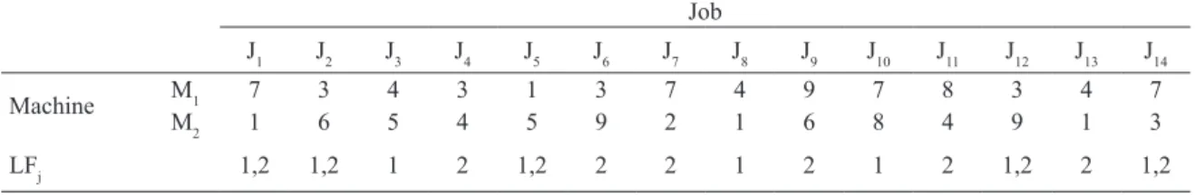
Let us first introduce a DPMASP example that will guide the exposition of the proposed heuristics. The example consists of fourteen jobs (n=14), three products (t=3), two factories (f=2) with two unrelated parallel machines in each factory (m=2). The assembly programs for each product are: N1={2, 7, 8}, N2={1, 3, 4, 10, 12, 13} and N3={5, 6, 9, 11, 14}, i.e., jobs 2, 7 and 8 must be finished in order to assemble product 1. Table 1 contains the job processing times on each machine at the production stage and eligibility constraints. Processing times for assembling products 1 to 3 are 3, 12 and 7, respectively.
Some additional notation is the following: A product sequence is represented by π, e.g., π = {2, 1, 3}. To assign all jobs belonging to the assembly program of product h to the unrelated parallel machines at the different factories, a job to machine-factory assignment method is needed. After the application of this assignment procedure we obtain a job to machine-factory sequence for product h, referred to πh, e.g., π1 = {0, 8; 7, 2}, π2 = {1-10, 3; 12, 4-13} and π3 = {14, 5; 6- 9, 11} as a possible job to machine-factory sequence for products of the example. At each πh, each factory is separated by “;”, each machine by “,” and the sequence of jobs at each machine is separated by “-”. A machine that is still empty (which can only occur in a partial solution) is denoted by “0” in its sequence. Following the previous example for π2 we have that jobs 1, 10 and 3 are assigned to the first factory. Jobs 1 and 10 are assigned to the first machine in this factory in this order and job 3 to the second machine. Since πh presents the job to machine-factory sequence of a single product h, πT, referred to as the final job sequence, is the concatenation of the different πh following the product sequence π. Following the previous example, πT = {1-10-14, 3-8-5; 12-7-6-9, 4-13-2-11}. Once
all jobs in the assembly program of a product h are completed in the production stage, it can be assembled on the assembly stage. Earliest assembling time of product h is denoted as Eh.
In this paper two methods are employed to construct the product sequence π. The first one uses the Shortest Processing Time heuristic (SPT). This dispatching rule is known to reduce the average number of jobs in the system, in-process inventories and average job tardiness (Stafford et al., 2005). We obtain the SPT order using the product assembly times and refer to this method as PS1. The second method, referred to as PS2, sorts the products in ascending order of the earliest assembling times (Eh).
In the method to make job to machine-factory assignments for products, we need first some additional notation. We refer to Uh to the set of unscheduled jobs of product h assembly program, i.e., those jobs not yet assigned to machines at factories. Skq is the set of jobs already scheduled at machine k inside factory q. With this in mind, the job to machine-factory assignment considers, for a product h, all jobs inside its assembly program, assigning first the unscheduled job with the earliest completion time at any machine in every eligible factory. More in details, we assign job j*∊U
h to
machine k* at factory q* satisfying:
, ,
, ,
argmin
j k q
k m q LF j Uj h pik pjk i Skq
! ! !
=
+
) ) )
!
"
' ,
1
/
The process is applied until all jobs in the assembly program of product h are scheduled.
Both proposed constructive heuristics consist of three main steps: In the first step, the product sequence π is constructed. In the second step, the jobs inside the assembly program of each product are assigned following the previous job to machine-factory assignment procedure, following the order of products given in π. Finally, in the third step the sequence of products for the assembly stage is obtained by sorting products according to Eh in
Table 1. Job processing times and factory eligibility constraints for the example.
Job
J1 J2 J3 J4 J5 J6 J7 J8 J9 J10 J11 J12 J13 J14
Machine M1 7 3 4 3 1 3 7 4 9 7 8 3 4 7
M2 1 6 5 4 5 9 2 1 6 8 4 9 1 3
ascending order. We propose two heuristics with identical second and third steps and with a different process to build the product sequence π in the first step.
4.1. Heuristics PJ1 and PJ2
In heuristic PJ1, PS1 is used to determine the product sequence π. After processing all jobs in the production stage, Eh for each product h is calculated. The product sequence on the assembly machine is updated by sorting Eh in ascending order and the final makespan is calculated. Pseudocode 1 explains PJ1 in detail:
Pseudocode 1: Outline of the PJ1heuristic. - Obtain product sequence, π, applying PS1 - Use the job to machine-factory assignment procedure to assign all jobs of each product following the product order in π
- Calculate earliest assembling time of each product h, Eh
- Determine the product sequence π on the assembly stage by sorting Eh in ascending order
The second heuristic PJ2 needs some careful explanation. It uses method PS2 in the first step to make the product sequence π. However, PS2 requires sorting products in increasing order of Eh. To calculate Eh, all jobs must be assigned to factories and machines. In heuristic PJ2, each product’s Eh is calculated in isolation. To calculate Eh of each product h, only jobs belong to product h are considered. Once Eh is calculated for all products, they are sorted in increasing order to form the product sequence π. This product sequence π is in turn used to apply again the job to machine-factory assignment for all products, which in the end gives us the final makespan.
The difference between heuristic PJ2, and the first heuristic PJ1, is just on the first step. As mentioned
before, heuristic PJ2, uses PS2 to construct π. Therefore, Pseudocode of heuristic PJ2 is not presented due to space constraints and because of its similarity with heuristic PJ1.
Note that if there are ties in the Eh of products, they are broken by taking the first product. Also the same rule is considered for breaking ties on the SPT rule which is used in heuristic PJ1 to calculate π.As a final note, and to enforce the technological constraint that no machine should be left empty, if after the application of any of the two proposed heuristics, any machine is left empty, we reassign to it the job with the smallest processing time at that machine. The two proposed heuristics are applied to the previous example in the next section for further clarification.
4.2. Heuristic application example
The example of Table 1 is used to detail heuristic PJ1 first. Products are first sorted according to shortest processing assembly times so π = {1, 3, 2}. In the second step, following the product order in π, first we assign jobs of product 1, to factories through the job to machine-factory assignment procedure. N1 = {2, 7, 8} so we first take job 2. The earliest completion time of this first job in all machines of all factories is 3. For job 7 is 2 (considering that it can only be assigned to factory 2) and for job 8 is 1 and can only be assigned to factory 1. The minimum is 1, which corresponds to the assignment of job 8 to the second machine of factory 1. Note that if there is a tie in the minimum completion time for the jobs, it is broken by taking the first job. We now have to consider the unscheduled jobs 2 and 7. We now calculate the earliest completion times of these two jobs at all machines of all eligible factories considering that job 8 is already assigned. These minimum completion times are 3 and 2 for jobs 2 and 7, respectively. Therefore job 7 is scheduled at factory 2 (the only eligible for this job) and to machine 2. Lastly, job 2 is scheduled with the earliest completion time of 3 at factory 1, machine 1. Note that we could have assigned this job to machine 1 of factory 2 with the same completion time, so we break ties by assigning jobs to the first
Table 2. Instance and factors for proposed instances.
Instance factor Symbol GA ValuesGB GC
Number of jobs n 10, 12, 14, 16, 18 20, 22, 24 200, 300, 400
Number of machines m 2, 3 2, 3, 4 5, 10, 15
Number of factories f 2, 3 2, 3, 4 4, 6, 8
machine and factory with equal completion time. After this procedure π1 = {2, 8; 0, 7}. Following the same process, the jobs in the assembly programs of products 3 and 2 are assigned to factories one after the other, resulting in the final job sequence πT = {2-12-3, 8-14-1-10; 5-6-4-13, 7-11-9}. The completion times of all jobs at the production stage are: C1 = 5, C2 = 3, C3 = 10, C4 = 7, C5 = 1, C6 = 4, C7 = 2, C8 = 1, C9 = 12, C10 = 13, C11 = 6, C12 = 6, C13 = 11 and C14 = 4. The earliest assembling time for products 1 to 3, by considering their respective assembly programs are: E1 = 3, E2 = 13 and E3 = 12, respectively. In the third step, the product sequence π on the assembly stage is updated by sorting Eh in ascending order, i.e., π = {1, 3, 2} and the Cmax of the application of PJ1 to this example is 31.
For the second heuristic PJ2 we calculate the Eh values for all products one by one with the job to machine-factory assignment procedure, the obtained sequences are π1 = {2, 8; 0, 7 } with E1 = 3, π2 = {12-10, 1-3; 4, 13} with E2 = 10 and π3 = {5, 14; 6, 11-9} with E3 = 10, so π = {1,2,3}. Note that there is a tie in the Eh of products 2 and 3 so again we break ties by taking the first product. Using this π we apply again the job to machine-factory assignment procedure obtaining πT={2-12-10, 8-1-3; 4-5-6-9, 7-13-14-11} with completion times for the jobs as: C1= 2, C2= 3, C3= 7, C4= 3, C5= 4, C6= 7, C7= 2, C8= 1, C9= 16, C10= 13, C11= 10, C12= 6, C13= 3 and C14= 6. In the third step, again products are sorted in increasing order of their respective Eh which are E1= 3, E2= 13 and E3= 16. Therefore, the updated product sequence for the assembly stage is π ={1, 2, 3} with a makespan of 32.
5. Computational evaluation
To test the proposed MILP model and constructive heuristics, six complete sets of instances have been generated. We consider different number of problem
characteristics to comprehensively evaluate and test the proposed approaches: Number of jobs (n), number of machines (m), number of factories (f) and number of products (t) are four controlled instance factors. Depending on the chosen values we have small, medium and large-sized instances, referred to as GA, GB and GC, respectively. The processing times of the jobs on each machine in the production stage, are generated following a random uniform distribution in the range [1, 99], as it is common in the scheduling literature. The last instance factor we consider is the distribution of the assembly processing times which are fixed as: U[|Nh|,49×|Nh|] and U[|Nh|,99×|Nh|]. These two distributions are referred to in short as 50, and 100, respectively. The final sets of instances are then denoted as GA50, GA100,…,GC100. For each combination of instance factors we have five replications. The combinations for each instance size are given in Table 2.
Therefore, the total number of instances is 300 for GA50 and another 300 for GA100 and 405 for every set in GB50 through GC100 resulting in a grand total of 2220 instances.
5.1. MILP model evaluation
The proposed MILP model is tested only on sets GA and GB given the impossibility to solve large instances. Two state-of-the-art commercial solvers are used, namely CPLEX 12.6 and GUROBI 5.6.3, which are, at the time of the writing of this paper, the latest versions available. Two different stopping times are tested with each solver: 900 and 3600 seconds. In total we have obtained 5640 results. All tests are performed in a high performance computing cluster with 30 blades, each one containing 16 GBytes of RAM memory and two Intel XEON E5420 processors running at 2.5 GHz. The 30 blade servers are used only to divide the workload since experiments are performed in virtualized Windows XP machines, each one with a virtualized processor
Table 3. Performance results for solvers and time limit for instance sets of GA50, GA100, GB50 and GB100.
Solver Instance setTime Limit GA 900s 3600s
50 GA100 GB50 GB100 GA50 GA100 GB50 GB100
CPLEX
% opt 96.67 98.00 79.50 87.40 97.00 98.33 81.72 88.39
% outm 0.00 0.00 2.46 1.72 0.00 0.00 12.34 6.41
GAP % 0.18 0.06 0.55 0.23 0.15 0.05 0.32 0.07
Av Time (sec.) 48.92 28.37 201.02 133.95 133.28 79.04 391.35 286.12
GUROBI GAP %% opt 95.670.29 98.000.07 74.561.15 81.970.51 97.000.21 98.670.05 77.030.82 84.440.37
with two cores and 2 GB of RAM memory. Therefore, since both CPLEX and GUROBI are parallel solvers, the two available threads at each virtual machine are used.
After solving the models with CPLEX and GUROBI, three possible outcomes are obtained. The first type is “optimal”, which means that an optimal solution with a given makespan value was obtained in the given maximum CPU time. The second type is “non-optimal”, meaning that a feasible integer solution was obtained within the time limit but it was not possible to demonstrate its optimality and the gap is reported. The third and last outcome is “out of memory”, by which the solver had an error and ran out of RAM memory, reporting a solution and a gap calculated with respect to the best obtained solution for that instance. In general, the solvers were able to find 294 (98.00%) and 297 (99.00%) optimal solutions in sets GA50 and GA100, respectively. For GB50 and GB100 the numbers are 338 (83.45%) and 363 (89.63%) for the 405 instances, respectively. The summarized results, according to the instance factors, type of solver and time limit, are presented in Table 3 for sets GA and GB. The reported values at the tables are the percentage of optimum solutions found (% opt), the percentage of cases with out of memory error (% outm), the average gap for non-optimal solution (GAP %) and the average CPU time in seconds (Av Time).
As we can see, the effect of the distribution of the assembly times at the assembly stage is much stronger than either the type of solver or CPU time limit. For group GA, instances with more disperse assembly times are easier to solve and also need less CPU time. As regards the comparison between CPLEX and GUROBI, for set GA we see comparable performance with slightly shorter CPU times for
CPLEX. For instance sets GB the differences between solvers are stronger. We see that GUROBI is much slower than CPLEX and has higher gap values. However, CPLEX reports out of memory errors that in some cases average more than 12% (GB50). So it is important to conclude that there is no clear winner for this problem between these two solvers. In total, the largest tested instances in sets GB have 24 jobs and 16 machines distributed in 4 factories so we can attest that the proposed mathematical model has an adequate performance.
5.2. Heuristics evaluation
The two proposed heuristics, PJ1 and PJ2, are now tested. The response variable is the Relative Percentage Deviation (RPD), measured as:
lg
RPD= A Bestsol-Bestsol sol#100
Where Bestsol is the best makespan obtained after all experimentation in this paper for any instance and Algsol is the makespan obtained by the heuristic. The heuristics are coded in C# and are compiled under Visual Studio 2010. The same computing platform used for the MILP evaluation is employed here. The average RPD values for the proposed heuristics are given in Tables 4, 5 and 6 for instances sets GA, GB and GC, respectively. All results are grouped by n and f. The average RPD values of CPLEX and GUROBI are reported as well for reference.
As can be observed, PJ2 is generally much better than PJ1 in all groups of instances, although the difference is not very big in the large instances. It is important to observe how in the largest instances in set GB of 24 jobs and 4 factories, PJ2, gives a very small gap of just 0.35% which indicates that PJ2 is a very capable
Table 4. Average Relative Percentage Deviation (RPD) of CPLEX, GUROBI and the proposed heuristics for instance sets
GA50 and GA100.
GA50 GA100
f×n CPLEX GUROBI PJ1 PJ2 CPLEX GUROBI PJ1 PJ2
2×10 0.00 0.00 9.52 3.26 0.00 0.00 2.21 0.46
2×12 0.00 0.00 8.24 4.04 0.00 0.00 3.58 1.76
2×14 0.00 0.00 8.29 3.36 0.00 0.00 4.50 0.62
2×16 0.00 0.00 9.31 4.59 0.00 0.00 4.30 1.16
2×18 0.00 0.21 7.27 3.90 0.00 0.00 3.34 1.23
3×10 0.00 0.00 5.10 2.59 0.00 0.00 1.09 1.24
3×12 0.00 0.00 4.72 1.43 0.00 0.00 1.85 0.98
3×14 0.00 0.00 4.51 1.71 0.00 0.00 1.51 0.28
3×16 0.00 0.00 4.79 1.39 0.00 0.00 2.63 0.72
3×18 0.00 0.00 4.04 1.34 0.00 0.00 2.15 0.78
heuristic with close to optimality performance. On average, PJ2 is below 1% RPD for instance groups GA and GB. For the large instances in GC it is not possible to calculate the optimum solution so we only have an overall picture were PJ2 always obtains the best solution. As a matter of fact and although not reported in detail here, among the 810 instances in GC50 and GC100, PJ2 is always better or equal than PJ1.
We report now on the CPU times of the proposed heuristics in Table 7. It has to be noted that CPU times are negligible, on the verge of being below the margin of error in measurements.
As can be seen, the average CPU times are below one tenth of a second for the largest instances in group GC. On average, PJ2 is relatively slower than PJ1 but on absolute terms the CPU times are very small. Although not shown here, the largest measured CPU time corresponds to heuristic PJ2 and has been 0.41 seconds. From this final evaluation and considering the relative RPD of PJ2 we can conclude that it is a capable and very fast heuristic.
Even though the observed differences are large in all cases for the proposed heuristics and very small for the two solvers, we carry out some statistical analyses in order to ascertain if the observed differences are indeed statistically significant. All results are examined with the Analysis of Variance (ANOVA) technique. ANOVA is a powerful parametric tool, which has been used in the last 10 years in the scheduling literature with great success. For the small instances there is no statistically significant difference in the performance of CPLEX and GUROBI and PJ2 is statistically better than PJ1. The detailed data is not reported for space reasons. For the medium sized-instances in set GB we observe the interaction between the distribution of the assembly processing times and tested methods in Figure 1. As can be seen, the results are similar to those of set GA. The differences between the proposed heuristics
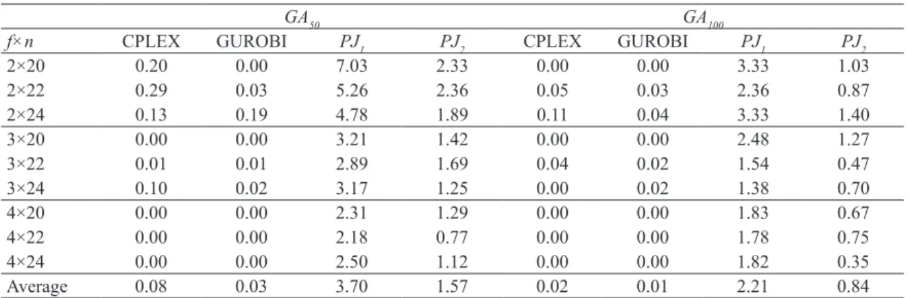
Table 5. Average Relative Percentage Deviation (RPD) of CPLEX, GUROBI and the proposed heuristics for instance sets
GB50 and GB100.
GA50 GA100
f×n CPLEX GUROBI PJ1 PJ2 CPLEX GUROBI PJ1 PJ2
2×20 0.20 0.00 7.03 2.33 0.00 0.00 3.33 1.03
2×22 0.29 0.03 5.26 2.36 0.05 0.03 2.36 0.87
2×24 0.13 0.19 4.78 1.89 0.11 0.04 3.33 1.40
3×20 0.00 0.00 3.21 1.42 0.00 0.00 2.48 1.27
3×22 0.01 0.01 2.89 1.69 0.04 0.02 1.54 0.47
3×24 0.10 0.02 3.17 1.25 0.00 0.02 1.38 0.70
4×20 0.00 0.00 2.31 1.29 0.00 0.00 1.83 0.67
4×22 0.00 0.00 2.18 0.77 0.00 0.00 1.78 0.75
4×24 0.00 0.00 2.50 1.12 0.00 0.00 1.82 0.35
Average 0.08 0.03 3.70 1.57 0.02 0.01 2.21 0.84
Table 6. Average Relative Percentage Deviation (RPD) of the proposed heuristics for instance sets GC50 and GC100.
f×n
GC50 GC100
PJ1 PJ2 PJ1 PJ2
4×200 0.13 0.00 0.07 0.00
4×300 0.12 0.00 0.05 0.00
4×400 0.11 0.00 0.06 0.00
6×200 0.09 0.00 0.04 0.00
6×300 0.08 0.00 0.05 0.00
6×400 0.08 0.00 0.04 0.00
8×200 0.06 0.00 0.03 0.00
8×300 0.08 0.00 0.03 0.00
8×400 0.05 0.00 0.04 0.00
Average 0.09 0.00 0.05 0.00
-0.3 0.7 1.7 2.7 3.7 4.7
A
ve
ra
ge
R
el
at
iv
e
Pe
rc
en
ta
ge
D
ev
ia
tio
n
PJ1 PJ2 CPLEX GUROBI
Assembly times distribution
50 100
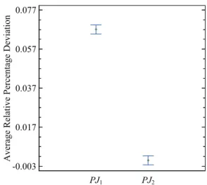
are large enough so as to be statistically significant whereas the differences in the performance of the solvers are not statistically relevant. As for the large instances in group GC we can only test the significance in the observed differences in the average RPD between the two heuristics. This is given in Figure 2.
-0.003 0.017 0.037 0.057 0.077
A
ve
ra
ge
R
el
at
iv
e
Pe
rc
en
ta
ge
D
ev
ia
tio
n
PJ1 PJ2
Figure 2. Means plot for the two heuristics in large instances (GC). All means have Tukey’s Honest Significant Difference (HSD) 95% confidence intervals.
As can be observed, PJ2 is statistically better than PJ1 even though the absolute difference between both proposed methods is practically small.
6. Conclusions and future research
In this paper we have studied an interesting combination of a distributed manufacturing problem with assembly operations. More specifically, we have presented a distributed unrelated parallel machines problem by which a number of factories, each one containing unrelated parallel machines have to manufacture jobs. All these jobs are later assembled into products in a factory with a single assembly machine. The objective is to minimize the
makespan in the assembly stage. Such a problem has been motivated and shown not to have been studied to date. We have presented a mathematical model and two constructive heuristics. The mathematical model has been comprehensively evaluated and tested using two state-of-the-art commercial solvers. Results have shown that we are able to solve optimally problems of up to 24 jobs and 16 machines distributed in 4 factories. The two proposed heuristics are inherently simple and at the same time report solutions very close to optimal in the cases for which the optimal solution has been obtained. Furthermore, for large instances, the performance is very good, obtaining solutions in less than half a second.
While the studied problem has many potential applications, it is very likely for additional constraints to appear in practice. For example, sequence dependent setup times at machines are ubiquitous in real industries. More complex assembly stages with parallel assembly machines, or assembly flowshops, might be of interest. Lastly, other objective functions, basically those based on due dates are worthy of additional studies. Furthermore, metaheuristic techniques might improve the results of the mathematical models and proposed heuristics in a significant way. We expect dealing with some of these ideas in future work.
Acknowledgements
The Spanish Ministry of Economy and
Competitiveness supports Rubén Ruiz,
under the project “RESULT-Realistic Extended Scheduling Using Light Techniques” (No. DPI2012-36243-C02-01). Carlos Andrés is partially supported by the project “Hybrid Methods for Horizontal Cooperation in Green Transportation and Logistics GreenCOOP” TRA2013-48180-C3-3-P from the Spanish Ministry of Economy and Competitiveness.
References
Chan, F. T. S., Chung, S. H., Chan, P. L. Y. (2005). An adaptive genetic algorithm with dominated genes for distributed scheduling problems.
Expert Systems with Applications, 29(2): 364–371. doi:10.1016/j.eswa.2005.04.009
Chan, F. T. S., Chung, S. H., Chan, P. L. Y., Finke, G., Tiwari, M. K. (2006). Solving distributed FMS scheduling problems subject to maintenance: genetic algorithms approach. Robotics and Computer-Integrated Manufacturing, 22(5-6): 493–504. doi:10.1016/j.rcim.2005.11.005 Elmaraghy, H., Schuh, G., ElMaraghy, W., Piller, F., Schönsleben, P., Tseng, M., Bernard, A. (2013). Product variety management. CIRP
Annals-Manufacturing Technology, 62(2): 629–652. doi:10.1016/j.cirp.2013.05.007
Hariri, A. M. A., Potts, C. N. (1997). A branch and bound algorithm for the two-stage assembly scheduling problem. European Journal of
Operational Research, 103(3): 547–556. doi:10.1016/S0377-2217(96)00312-8
Hatami, S., Ruiz, R., Andrés-Romano, C. (2013). The distributed assembly permutation flowshop scheduling problem. International Journal
of Production Research, 51: 5292–5308. doi:10.1080/00207543.2013.807955
Jia, H. Z., Fuh, J. Y. H., Nee, A. Y. C., Zhang, Y. F. (2002). Web-based multi-functional scheduling system for a distributed manufacturing environment. Concurrent Engineering: Research and Applications, 10(1): 27–39.
Jia, H. Z., Nee, A. Y. C., Fuh, J. Y. H., Zhang, Y. F. (2003). A modified genetic algorithm for distributed scheduling problems. Journal of
Intelligent Manufacturing, 14(3-4): 351–362. doi:10.1023/A:1024653810491
Jia, H. Z., Fuh, J. Y. H., Nee, A. Y. C., Zhang, Y. F. (2007). Integration of genetic algorithm and Gantt chart for job shop scheduling in distributed manufacturing systems. Computers & Industrial Engineering, 53(2): 313–320. doi:10.1016/j.cie.2007.06.024
Lee, C. Y., Cheng, T. C. E., Lin, B. M. T. (1993). Minimizing the makespan in the 3-machine assembly-type flowshop scheduling problem.
Management Science, 39(5): 616–625. doi:10.1287/mnsc.39.5.616
Lenstra, J. K., Rinnooy Kan, A. H. G., Brucker, P. (1977). Complexity of machine scheduling problems. Annals of Discrete Mathematics, 1:343–362. doi:10.1016/S0167-5060(08)70743-X
Lin, S. W., Ying, K. C., Huang, C. Y. (2013). Minimising makespan in distributed permutation flowshops using a modified iterated greedy algorithm. International Journal of Production Research, 51(16): 5029–5038. doi:10.1080/00207543.2013.790571
Lin, Y., Li, W. (2004). Parallel machine scheduling of machine-dependent jobs with unit-length. European Journal of Operational Research, 156(1): 261–266. doi:10.1016/S0377-2217(02)00914-1
Mahdavi, I., Shirazi, B., Cho, N., Sahebjamnia, N., Ghobadi, S. (2008). Modeling an e-based real-time quality control information system in distributed manufacturing shops. Computers in Industry, 59(8): 759–766. doi:10.1016/j.compind.2008.03.005
Naderi, B., Ruiz, R. (2010). The distributed permutation flowshop scheduling problem. Computers & Operations Research, 37(4): 754–768. doi:10.1016/j.cor.2009.06.019
Naderi, B., Ruiz, R. (2014). A scatter search algorithm for the distributed permutation flowshop scheduling problem. European Journal of
Operational Research, 239(2): 323–334. doi:10.1016/j.ejor.2014.05.024
Sluga, A., Butala, P., Bervar, G. (1998). A multi-agent approach to process planning and fabrication in distributed manufacturing. Computers
& Industrial Engineering, 35(3-4): 455–458. doi:10.1016/S0360-8352(98)00132-6
Stafford, E. F., Tseng, F. T., Gupta, J. N. D. (2005). Comparative evaluation of MILP flowshop models. Journal of the Operational Research
Society, 56(1): 88–101. doi:10.1057/palgrave.jors.2601805
Sun, X., Morizawa, K., Nagasawa, H. (2003). Powerful heuristics to minimize makespan in fixed, 3-machine, assembly-type flowshop scheduling. European Journal of Operational Research, 146(3): 499–517. doi:10.1016/S0377-2217(02)00245-X
Sung, C. S., Kim, H. A. (2008). A two-stage multiple-machine assembly scheduling problem for minimizing sum of completion times.
International Journal of Production Economics, 113(2): 1038–1048. doi:10.1016/j.ijpe.2007.12.007
Wang, S. Y., Wang, L., Liu, M., Xu, Y. (2013). An effective estimation of distribution algorithm for solving the distributed permutation flowshop scheduling problem. International Journal of Production Economics, 145(1): 387–396. doi:10.1016/j.ijpe.2013.05.004