Rainfall analysis using conventional and non-conventional rainfall information on monthly scale

Full text

(1)Atmósfera 23(2), 141-164 (2010). Rainfall analysis using conventional and non-conventional rainfall information on monthly scale S. G. NARKHEDKAR, S. K. SINHA and P. MUKHOPADHYAY Indian Institute of Tropical Meteorology, Dr. Homi Bhabha Road, Pashan, Pune - 411 008 Corresponding author: S. G. Narkhedkar; e-mail: narkhed@tropmet.res.in Receibed September 26, 2009; accepted january 12, 2010 RESUMEN El objetivo de este trabajo es describir la técnica utilizada para crear el análisis integrado de precipitación sobre la India y su región adyacente (1.5 a 35.5º N y 63.5 a 97.5º E). La técnica es probada en campos mensuales de precipitación para un período de monzón de dos años (2001 y 2003) en rejillas de 1º x 1º de latitud-longitud, combinando las estimaciones de precipitación de diferentes fuentes: satelitales, de pluviómetros y de un modelo numérico de predicción climática. Primero, para reducir el error aleatorio de las estimaciones de satélite y del modelo de predición climática, éstas se combinan de forma lineal con base en el método de estimación máxima más probable. En este caso, el peso de cada componente es inversamente proporcional a los cuadrados de los errores aleatorios individuales. El peso es determinado comparando los componentes con el análisis pluviométrico correspondiente. Como el análisis combinado tiene desviaciones de las fuentes de los datos individuales, se combina con el análisis basado en las observaciones pluviométricas. Se observa que el análisis integrado producido es más cercano a las observaciones que las fuentes individuales. Se observa también que la magnitud y distribución de la precipitación orográfica fuerte a lo largo de los Gaths occidentales de la India es muy diferente y más realista cuando se compara con los datos del Global Precipitation Climatology Project (GPCP) y los del Climate Prediction Center (CPC) Merged Analysis of Precipiatation (CMAP). Cuando se compara el análisis integrado con el del India Meteorological Department, se encuentra que aquel muestra una correlación mayor que las predicciones de satélite y del modelo de precipitación. De los resultados se concluye que este estudio tiene resultados prometedores y que los análisis pueden utilizarse para evaluar modelos de simulación que sirvan como base para vigilancia en tiempo real. Asimismo, se podrán generar bases de datos de largo plazo en rejillas de alta resolución para escalas diaria y mensual, lo que a su vez podrá ser utilizado para estudiar la variabilidad espacial y temporal de la precipitación sobre la India y su región adyacente. ABSTRACT The aim of this paper is to describe the technique used to create the merged analysis of rainfall over the Indian and adjoining region (1.5º to 35.5º N and 63.5º to 97.5º E). The technique is tested for monthly gridded fields of rainfall for a 2-year monsoon period (2001 and 2003) on a 1º x 1º latitude-longitude grid by merging rainfall estimates from different sources, viz satellite based estimates, rain gauge analysis and numerical weather prediction model rainfall. First, in order to reduce the random error involved in the satellite rainfall estimates and the model predictions, satellite and model estimates are combined linearly based on a maximum likelihood estimate method. In this case the weight for each component is inversely proportional to the squares of the individual random errors. The weight is determined by comparing the components with the concurrent gauge analysis. As the combined analysis contains bias from the individual input data sources, the combined analysis is then blended with the analysis based on gauge observations. It is seen that the merged analysis produced here is closer to the observations than the individual sources. It is observed.

(2) 142. S.G. Narkhedkar et al.. that the magnitude and distribution of the orographic heavy rainfall along the Western Ghats of India is very different and more realistic compared to the Global Precipitation Climatology Project (GPCP) and the Climate Prediction Center (CPC) Merged Analysis of Precipitation (CMAP). When compared with the India Meteorological Department analysis, it is found that the merged analysis shows higher correlation than the satellite and model predicted rainfall. From the results it can be concluded that this study has shown promising results and the analyses can be used as a bench mark for evaluating model simulations which serves as a basis for real-time monitoring. Based on these promising results, long term datasets on high resolution grid for daily and monthly scale over Indian and adjoining region will be generated, which in turn can be used to study spatial and temporal variability of rainfall over Indian and adjoining region. Keywords: Gauge data, satellite estimates, NWP model, merged analysis, CMAP, GPCP.. 1. Introduction Rainfall is one of the most important and at the same time one of the most difficult meteorological/ hydrological parameter on which the economy of India depends. There has been increasing operational demand for daily/monthly rainfall analysis for a wide range of applications extending from the real time monitoring and prediction of flood events, climate analysis (Janowiak and Arkin, 1991), climate diagnostic study (Arkin and Xie, 1994), model verification (Gates, 1992) and global energy and water budget studies (WMO, 1993). The task of quantifying the distribution is complicated by the fact that no single technique exists to estimate monthly global/regional rainfall, despite the fact that rain and snow play an important role in the global meteorological cycle and the affairs of humans. The global and regional climate modeling community requires regional rainfall data for verifying the regional details derived from the model simulations. Daily and monthly rainfall datasets are useful for studying intraseasonal and interannual variations in the Indian summer monsoon (Kripalani et al., 1991). Among the different scientific groups who worked on preparing rainfall analysis, rainfall analysis by Huffman et al. (1997) under the Global Precipitation Climatology Project (GPCP), and the Climate Prediction Center (CPC) Merged Analysis of Precipitation (CMAP) by Xie and Arkin (1997) are the two important data sets, which have been utilized in a wide range of applications, including weather/climate monitoring, climate analysis, numerical model verifications and hydrological studies. After Adler et al. (1993, 1994) pioneering work in the area of merging different rainfall analysis, merging technique has gained wide importance. Generally, three kinds of data sources viz. gauge observations, estimates based on satellite observations and numerical model predictions are combined to produce rainfall analysis. But it is not sufficient to simply assemble the different rainfall estimates. The rain gauge observations have the longest recording period and are the only sources that are obtained through direct measurement. Rain gauge observations yield relatively accurate point measurements of rainfall, but suffer from sampling error in representing area means. Satellite radiance (infrared and microwave) data is being used to retrieve rainfall information over many parts of globe, but the estimates made from satellite observations contain non-negligible random error and bias. The rainfall distributions produced by various numerical models exhibit relatively high quality in mid- and high latitudes, but perform more poorly over most tropical areas (Arpe, 1991). Xie and Arkin (1995) found at least three important deficiencies in the individual rainfall sources: 1) incomplete coverage, 2) significant random error and 3) non-negligible bias. Thus it is necessary to improve the quality of the individual data sources and to merge them appropriately so as to take advantage of the strengths of each source..

(3) Rainfall analysis using conventional and non-conventional data. 143. Rainfall analysis prepared under GPCP is another very useful and widely utilized dataset. GPCP (Huffman et al., 1997) provides global monthly rainfall on a 2.5º latitude-longitude grid by merging rain gauge observations with multisatellite estimates of rainfall to take advantage of the strength of each dataset. Over land, bias in the multisatellite analysis is adjusted by gauge analysis. Over ocean no adjustment is made. Finally the gauge and multisatellite analyses are merged using the inverse error-weighting technique to form final GPCP analysis. Currently GPCP provides global monthly rainfall on a 1º latitude-longitude grid. Xie and Arkin (1996) developed a merging algorithm which combines five kinds of monthly rainfall datasets. Gauge observations, satellite estimates from infrared (IR), microwave (MW) scattering and MW-emission observations and numerical model predictions are used as input components. The merging of the individual data sources is conducted in two steps. First, for reducing the random error three satellite estimates and the model predicted rainfalls are linearly combined, based on a maximum likelihood estimation method in which the weighting coefficients are inversely proportional to the square of the individual random errors determined by comparing with the concurrent gauge-based analysis. It is expected that the linear combination of these datasets will have smaller random errors than any of these individual sources. Since output of the first step contains bias from the individual input data sources, in the second step the output of the first step is blended with the gauge-based analysis using the method of Reynolds (1988). The output of the first step defines the relative distribution or the “shape” of the field, while the gauge data determines the amplitude of the rainfall field. Xie and Arkin (1997) applied this algorithm to produce global monthly rainfall on a 2.5º latitude-longitude grid, for an 18-month period from July 1987 to December 1988, by merging gauge observations and a number of satellite estimates. The authors have named this dataset as Climate Prediction Center Merged Analysis of Precipitation (CMAP). Although both the algorithms produce and depict useful global monthly rainfall, there are significant differences in the methodologies by which the various input data are merged. As both the datasets used the same GPCC (Global Precipitation Climatology Center) data, they agree well over land. While over some of tropical oceanic areas CMAP is 20 to 50% wetter than GPCP. GPCP is wetter than CMAP polewards of 45º (oceanic areas). Over Indian region, some studies have been carried out for producing rainfall analysis by using both conventional as well as non-conventional rainfall data simultaneously. Mitra et al. (2003) made daily rainfall analysis over Indian monsoon region. They corrected the satellite (INSAT1D) estimates using the weighted mean of the differences between the observed and interpolated values over gauge location. They carried out the analysis on a 1.5º latitude-longitude grid using successive correction method. They found that the magnitude and distribution of orographic rainfall along the west coast of India is high and more realistic compared to both CMAP and GPCP. IMD prepared 1º x 1º latitude-longitude gridded daily rainfall dataset over the Indian region for the period (1951-2003) using Shepard (1968) interpolation scheme (Rajeevan et al., 2006). They studied the active and break period during the southwest monsoon season (June to September), using this gridded rainfall datasets, and found that the break periods identified were comparable with earlier studies. Sinha et al. (2006) made rainfall analysis over Indian and adjoining region using Barnes technique on a 0.25º latitude-longitude grid for five days of August 1994, when a depression was formed over Bay of Bengal. Roy Bhowmik and Das (2007) made objective analysis for 2001 and 2003 (June-August) by merging rain gauge observations and satellite estimates. In order to.

(4) 144. S.G. Narkhedkar et al.. take the advantage of gauge data over land and satellite estimate over ocean, they combined the gridded rainfall data over land and the satellite rainfall estimates over ocean. Xie et al. (2007) made daily rainfall analysis on a 0.5º latitude-longitude grid over East Asia (5º to 60º N, 65º to 155º E) for a 26-yr period from 1978 to 2003. Narkhedkar et al. (2008) applied Barnes scheme to interpolate irregularly distributed daily rainfall data on to a regular grid on spatial resolution of 0.25º latitude-longitude. They combined daily rainfall derived from INSAT IR radiances and raingauge observations to produce this analysis adding some objectively determined constraints viz. 1) weights are determined as a function of data spacing, 2) in order to achieve convergence of the analyzed values three passes through the data are considered and there is automatic elimination of wavelengths smaller than twice the average data spacing. The rainfall variations in the global gauge based and merged analysis do not always match with those in the regional gauge-based analysis, because of the differences in the gauge station data and interpolation algorithms used in defining the gauge analysis (Xie et al., 2003). Earlier analyses on regional domains were created over the CONUS-México domain (Higgins and Shi, 2000) on a 0.25º latitude-longitude grid. Over South America (Shi et al., 2001; Silva et al., 2007) on a 1º latitude-longitude grid and over East Asia (Xie et al., 2007) on a 0.5º latitude-longitude grid analyses were made by interpolating the Global Telecommunication System (GTS) and regional station data. Although all the above mentioned datasets available over the globe have proved their utility, over Indian and adjoining region there is hardly any grid point dataset available to study the variability of the rainfall featuring regional characteristics. IMD data is available and is proved to be very good over land region. IMD has used only rain gauge data. Due to the advent of various remote sensing data sources, it is the need of the hour to make maximum utilization of the datasets available from various sources, viz. satellites, radars, NWP model outputs etc. GPCP and CMAP datasets have proved to be very useful over the global scale, but due to their low resolution (2.5º x 2.5º) they cannot capture the regional features in rainfall analyses that have a lot of variability in time and space. In the last few years, preparation of gridded data sets for Asian monsoon region has caught the attention of meteorologists and hydrologists. Motivated by the increasing demand of high resolution merged rainfall analysis over Indian and adjoining region, this study has been taken up to produce daily and monthly rainfall analyses on 1º latitude-longitude grid for the monsoon season (June-September). In doing so, the technique developed by Xie and Arkin (1996) has been followed. The merged data will be useful in studying the spatial and temporal variability of rainfall during the monsoon season over Indian and adjoining region. To start with, rainfall analyses of 2001 and 2003 using INSAT 1-D and Kalpana-1 estimates and WRF model estimates along with rain gauge data are presented here. 2. Data sources The daily rain gauge analysis data over land region at 1º latitude-longitude for the period 2001 and 2003 for the monsoon months (June-September) are provided by IMD. IMD utilized 1803 observations out of 6329 for which a minimum of 90% data are available for analysis (Rajeevan et al., 2006). They used Shepard (1968) scheme for interpolation. Daily quantitative precipitation estimates (QPE) derived from satellite on a 1º latitude-longitude for 2001 and 2003 were provided by Satellite Meteorology Division of IMD. In the year 2001,.

(5) Rainfall analysis using conventional and non-conventional data. 145. QPE data was available from Indian National Satellite System geostationary satellite INSAT-1D. IR is based on the Geostationary Operational Environmental Satellite (GOES) Precipitation Index (GPI) technique (Arkin and Mesiner, 1987). The rainfall estimates were available in real time for the defined region on a 1º latitude-longitude grid. The satellite was defunct in 2002. For the year 2003, QPE data available from INSAT-Kalpana–1 has been used for the analysis. The data is based on the same technique which has been used for INSAT-1D. Every 3 hour rainfall is computed at 1º latitude-longitude grid. Then it is accumulated for total 24 hours (8 times) valid at 3 UTC. Numerical model rainfall forecasts (24 h accumulated) produced by the Weather Research and Forecasting model WRF with version 2.2 run at Indian Institute of Tropical Meteorology (IITM) is used in this study. Its horizontal resolution is 27 km (single domain) and vertical resolution is 31 km with terrain following sigma coordinate. Model top is at 50 hPa. In model physics the cumulus scheme of Betts Millar Janjic is used while micro physics is of Purdue Lin. Surface layer is Monin-Obukhov similarity. Planetary boundary layer is applied following Yansei University (YSU) scheme. Rapid radiative transfer Model (RRTM) is used as longwave radiation whereas for shortwave radiation, Dudhia shortwave scheme is applied. For running the model, interpolated values from NCEP reanalysis 2.5º latitude-longitude grid are used as initial condition. Lateral boundary conditions are the updated 6 hour data from NCEP reanalysis. Model is integrated from 0000 UTC 01 May - 0000 UTC 01 October for both 2001 and 2003 over the domain 62.10 to 104.00º E and 1.00 to 36.00º N. The model forecast is then interpolated to 1º latitude-longitude for merging with the satellite estimate and gauge analysis. The domain for current study is from 63.5 to 97.5º E longitude and 1.5 to 35.5º N latitude, cast on a 1º latitude-longitude grid. 3. Salient features of Indian summer monsoon 2001: The rainfall activity during the southwest (SW) monsoon season 2001 was well distributed in space and time. Total seasonal monsoon rainfall over the country as a whole was 91 % of its long period average. The eastern parts of the country received very good amount of rainfall throughout the season, the activity was in the first half of the season in northern and western parts and over peninsula, it was good at the end of the season. Off-shore trough along different parts of west coast persisted on most of the days during the monsoon period. 2003: The rainfall activity during the southwest (SW) monsoon season 2003 was also well distributed in space and time like 2001. Total seasonal monsoon rainfall over the country as a whole was 102 % of its long period average. Off-shore trough was formed along different parts of the west coast on most of the days of monsoon period. 4. Merging methodology As discussed earlier, it is not sufficient only to assemble the different kind of rainfall estimates. To form a weighted combination of various rainfall estimates, it is necessary to compute errors in each field. Due to the unavailability of error estimates, following Xie and Arkin (1996) the error estimates are computed and the merged analysis experiment is conducted over Indian and adjoining region. As mentioned earlier the merging algorithm consists of two parts. In the first part satellite estimates and model rainfall are combined and in the second part combined analysis is.

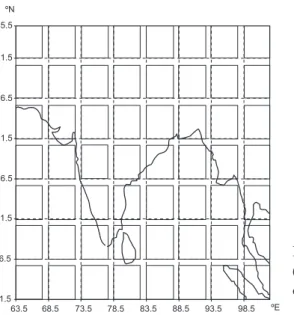
(6) 146. S.G. Narkhedkar et al.. then blended to produce final merged analysis. As the merging analysis is being carried out over Indian and adjoining region, which comprises land area as well as oceanic region, the merging analysis is carried out separately for land and ocean. In this experiment reference field used for land is gauge analysis on 1º latitude-longitude produced by IMD, and over oceanic region CMAP analysis available on a 2.5º latitude-longitude is used as a reference field. This CMAP analysis was further interpolated on 1º latitude-longitude using routine interpolation technique. Both the data sets have been tested extensively in various studies by different scientists. 4.1 Combining algorithm Let us assume that the observational error (σi) is random, unbiased, normally distributed and the observation errors for different kinds of observations are independent. Then the maximum likelihood estimate of C (combined field) is expressed as n. C=. Wi Fi, . (1). i=1. where Fi and Wi are the individual observations and the weighting function, respectively. The weighting function Wi is given by 2 i. Wi =. −2 i. . . (2). The expected error variance of C is given by. E2 =. [. −2 i. ]. −1. . . (3). Thus, the maximum likelihood estimate of rainfall at a given grid area is a linear combination of the individual data sources, in which the weighting coefficients are inversely proportional to the observational error variance of each source. Since the individual estimates (satellite and model prediction) contain error and bias, the observational errors in equations (2) and (3) are defined as the random errors and are computed as follows. As shown in Figure 1, the entire region of our analysis is divided into 49 blocks each having a dimension of 5º x 5º. These blocks are distributed in such a way that there are seven blocks in each horizontal and vertical direction. This has been done with the aim to calculate random errors representing the homogeneous area. First we computed the mean difference between source field and IMD analysis (reference field), for a 5º x 5º array of grid areas centered on the target grid area and then this mean difference is subtracted from the source field over that array to produce modified source field. The random error is then defined as the root mean square difference between the modified source field and the IMD analysis on the same 5º x 5º array. As can be seen from Figure 1 near the coastlines, the 5º x 5º array is not completely filled by the IMD analysis and hence the subset for which values are available is used. Using these random errors, the distribution of the combined analysis C over the Indian land region is constructed by calculating the maximum likelihood estimate from individual sources using equations (1) and (2)..

(7) Rainfall analysis using conventional and non-conventional data. 147. ºN 35.5 31.5. 26.5. 21.5. 16.5. 11.5. Fig. 1. (7 x 7 = 49) blocks constructed over analysis area (1.5 to 35.5º N and 63.5 to 97.5º E) each having dimension of 5º x 5º.. 6.5. 1.5 63.5. 68.5. 73.5. 78.5. 83.5. 88.5. 93.5. 98.5. ºE. 4.2 Blending of the combined analysis Combined analysis thus obtained, contains bias passed through from the satellite estimate and model prediction. Hence in the second step to remove the bias the combined analysis (C) is blended with IMD based gauge analysis (G). Blending algorithm of Reynolds (1988) is used in this experiment by assuming that: a) the shape of the blending analysis B satisfy Poisson’s equation ∇2 B = Q, (4) b) the forcing term Q in equation (4) is computed from the combined analysis C Q = ∇2 C, (5) c) the boundary condition is defined such that the blending analysis B at the boundary is identical to gauge analysis (G) B = G at the boundary. (6) The blending analysis B is thus obtained by numerically solving the equation (4) using relaxation technique. The final product generated using the above algorithm still contains bias. It is not possible to remove all bias, because the bias in the gauge-based analysis will remain in the merged analysis. The merging algorithm described in the above section is for the Indian land region where IMD-based gauge analysis is taken as reference field. Similar procedure is adopted for the merged analysis over oceanic area, where the CMAP analysis on 1° latitude-longitude grid is used as reference field. 5. Results of analysis experiment To evaluate the performance of the algorithm, which is based on the Xie and Arkin (1996) technique, and the quality of the merged analysis, we computed the correlation and root mean square (RMS) errors of individual sources and the merged analysis with respect to reference (IMD) analysis. The correlations (CC) for the individual sources and the merged analysis, and the respective RMS errors (RMSE) for both the years (2001 and 2003), are shown in Table I..

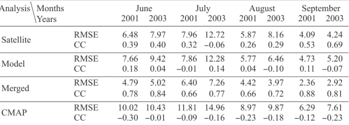
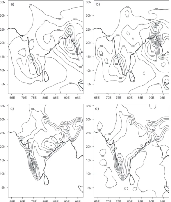
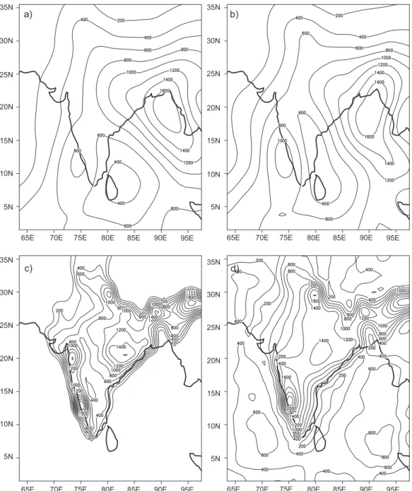
(8) 148. S.G. Narkhedkar et al.. Table I. RMS errors (mm) and correlation coefficients as compared to the IMD analysis (reference analysis) only over land region. Analysis Months Years. June 2001 2003. July 2001 2003. August 2001 2003. September 2001 2003. 5.87 0.26. 4.09 0.53. Satellite. RMSE CC. 6.48 0.39. 7.97 0.40. 7.96 12.72 0.32 -0.06. Model. RMSE CC. 7.66 0.18. 9.42 0.04. 7.86 12.28 -0.01 0.14. Merged. RMSE CC. 4.79 0.78. 5.02 0.84. CMAP. RMSE CC. 10.02 10.43 -0.30 -0.01. 6.40 0.66. 7.26 0.77. 11.81 14.96 -0.09 -0.16. 8.16 0.29. 4.24 0.69. 5.77 6.46 0.04 -0.10. 4.73 5.20 0.11 -0.07. 4.42 0.66. 2.36 0.88. 3.97 0.72. 8.97 9.87 -0.23 -0.18. 2.92 0.81. 6.29 7.61 -0.12 -0.23. From Table I it is found that the correlations for the merged analysis are higher than the CMAP analysis and the individual data sources when compared with IMD analysis. Satellite estimates show similar correlations (below 0.5) throughout the season, except September when they are 0.53 and 0.69 for 2001 and 2003, respectively. In September rainfall activity was subdued. RMS errors are ranging from 4.0 to 12.7. Correlations of model rainfall are very poor (below 0.18) and as expected RMS errors are higher (ranging from 4.7 to 12.3). Similar trend is seen for CMAP analysis where the correlations are very poor (below ± 0.3) and the RMS errors are at higher (6.3 to 14.9) side. But after merging the satellite and model rainfall the merged rainfall has produced improved analysis. The correlation has increased up to 0.88 and RMS errors are reduced considerably (from 7.26 to 2.35). Figure 2 (a-d) shows the rainfall distribution of satellite estimate for June-September (2001). The model rainfall distribution for June-September 2001 is shown in Figure 3(a-d). Shown in Figure 4(a-d) is the monthly rainfall distributions from GPCP, CMAP, IMD and merged analyses for June 2001. Similarly rainfall distributions from GPCP, CMAP, IMD and merged analyses for July, August and September 2001 are shown in Figures 5(a-d), 6(a-d) and 7(a-d), respectively. It is seen from Figures 4(d) to 7(d) that the pattern of the rainfall distribution of merged analysis resembles with the IMD analysis at most grid areas over central India, southern peninsula and west-coast of India where gauge network is denser. It is also observed that the merged analysis is more smoother and has produced slightly lesser rainfall values over most part of the Indian land region as compared to IMD analysis. Over other Indian regions like north India, foothills of Himalayas, northeast region where gauge data is sparse, spatial distribution of merged analysis is derived from the satellite estimates and model prediction. Thus the merged analysis is able to take advantage of the strengths of the individual sources. The amplitude of the merged analysis is controlled by gauge-based reference field. The merged monthly rainfall analysis for the four months for 2001 (Figs. 4d to 7d) are compared with the IMD analysis (Fig. 4c to 7c), and also with the GPCP (Fig. 4a to 7a) and CMAP (Fig. 4b to 7b) analyses to assess the utility of the merged analysis. IMD analysis (June, 2001) shows rainfall amounts from 200 to 700 mm along the west-coast of India. Merged analysis also shows similar rainfall amounts along the west-coast of India. Higher rainfall experienced along the east coast, west coast and over central India in the merged analysis is not seen in the GPCP analysis (Fig. 4a) and CMAP analysis (Fig. 4b). Over the head of the Bay of Bengal both the analyses (GPCP and CMAP) are showing rainfall contours of 800 and 1100 mm, which is very high compared to the IMD analysis. Areal.

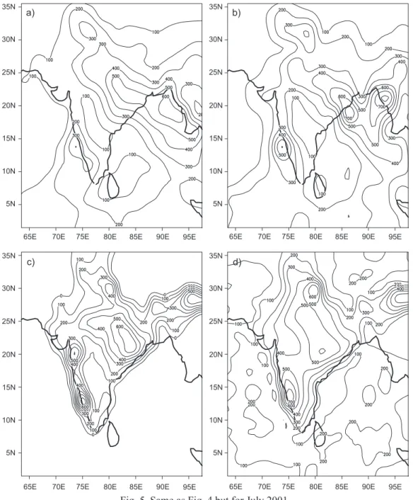
(9) 149. Rainfall analysis using conventional and non-conventional data. 35N. 35N. a). 30N. 30N. 25N. 25N. 20N. 20N. 15N. 15N. 10N. 10N. 5N. 5N. 65E 35N. 70E. 75E. 80E. 85E. 90E. 65E. 95E 35N. c). 30N. 30N. 25N. 25N. 20N. 20N. 15N. 15N. 10N. 10N. 5N. 5N. 65E. 70E. 75E. 80E. 85E. 90E. 95E. b). 70E. 75E. 80E. 85E. 90E. 95E. 70E. 75E. 80E. 85E. 90E. 95E. d). 65E. Fig. 2. Monthly analyses of satellite estimated rainfall (mm) for the months of a) June, b) July, c) August and d) September for 2001.. averaged rainfall over Mangalore is 700 mm of rainfall (IMD analysis for June 2001, Fig. 4c) as can be seen in the merged analysis (Fig. 4d). In the month of July when the monsoon is well set, IMD analysis shows (Fig. 5c) 100 mm or more rainfall over Indian region. Again in this month also, west coast shows rainfall between 200 to 700 mm. A closed contour of 600 mm is seen over east part of central India. Along the monsoon trough 400 mm of rainfall is reported. The merged analysis also shows similar features of rainfall analysis along the west coast. Along the foothills of Himalayas the.

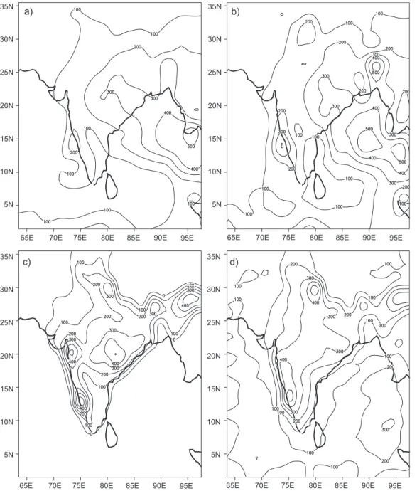
(10) 150. S.G. Narkhedkar et al.. 35N. 35N. a). 30N. 30N. 25N. 25N. 20N. 20N. 15N. 15N. 10N. 10N. 5N. 5N. 65E 35N. 70E. 75E. 80E. 85E. 90E. 65E. 95E 35N. c). 30N. 30N. 25N. 25N. 20N. 20N. 15N. 15N. 10N. 10N. 5N. 5N. 65E. 70E. 75E. 80E. 85E. 90E. 95E. b). 70E. 75E. 80E. 85E. 90E. 95E. 70E. 75E. 80E. 85E. 90E. 95E. d). 65E. Fig. 3. Same as Fig. 2 but for model predicted rainfall.. patterns of rainfall analysis of merged and IMD analyses are almost the same. GPCP and CMAP both show 300 and 500 mm of rainfall, respectively, along the west coast. In the month of August 2001, GPCP (Fig. 6a) and CMAP (Fig. 6b) both underestimate rainfall over the west coast of India. Merged analysis (Fig. 6d) shows maximum of 500 mm of rainfall on the west. IMD analysis (Fig. 6c) also shows the same feature. Along the foothills of Himalayas heavy rainfall (Fig. 6d) about 500 mm is seen in the merged analysis. IMD analysis (Fig. 6c) produced high rainfall but its magnitude is less compared to merged analysis. The GPCP analysis is very smooth.

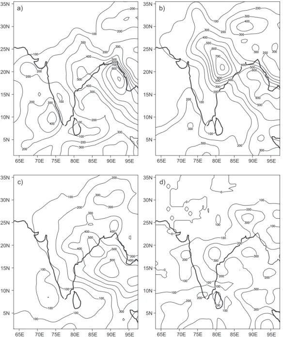
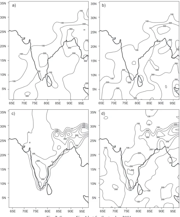
(11) 151. Rainfall analysis using conventional and non-conventional data. 35N. 35N. a). 30N. 30N. 25N. 25N. 20N. 20N. 15N. 15N. 10N. 10N. 5N. 5N. 65E 35N. 70E. 75E. 80E. 85E. 90E. 65E. 95E 35N. c). 30N. 30N. 25N. 25N. 20N. 20N. 15N. 15N. 10N. 10N. 5N. 5N. 65E. 70E. 75E. 80E. 85E. 90E. 95E. b). 70E. 75E. 80E. 85E. 90E. 95E. 70E. 75E. 80E. 85E. 90E. 95E. d). 65E. Fig. 4. Monthly rainfall (mm) analysis for June 2001 from a) GPCP, b) CMAP, c) IMD and d) merged analyses.. and is not able to capture this feature very well. In September when the monsoon starts withdrawing, the rainfall reduces and the associated rainfall pattern withdraws from the northwest India towards the south (Fig.7c). Similar features are also seen in GPCP (Fig.7a), CMAP (Fig.7b) and merged (Fig.7d) analyses. IMD (Fig.7c) and merged (Fig. 7d) analyses both show 200 mm rainfall over coastal Kerala. Merged analysis (Fig. 7d) shows about 300 mm rainfall along the foothills of Himalayas, similar as IMD analysis. Both the analyses (IMD and merged) show identical amounts and also the shape of.

(12) 152. S.G. Narkhedkar et al.. 35N. 35N. a). 30N. 30N. 25N. 25N. 20N. 20N. 15N. 15N. 10N. 10N. 5N. 5N. 65E 35N. 70E. 75E. 80E. 85E. 90E. 65E. 95E 35N. c). 30N. 30N. 25N. 25N. 20N. 20N. 15N. 15N. 10N. 10N. 5N. 5N. 65E. 70E. 75E. 80E. 85E. 90E. 95E. b). 70E. 75E. 80E. 85E. 90E. 95E. 70E. 75E. 80E. 85E. 90E. 95E. d). 65E. Fig. 5. Same as Fig. 4 but for July 2001.. the analysis is the same in the horizontal direction along the latitude belt, 27º N. This is not seen in the GPCP (Fig. 7a) and CMAP (Fig.7b) analyses. These regional features are very much important and are not being captured by the CMAP and GPCP analyses, which are generated on the global scale. Figure 8 (a-d) shows the seasonal total rainfall for GPCP, CMAP, IMD and merged analyses, respectively, for 2001. GPCP and CMAP show maximum of 800 and 1000 mm of rainfall over west coast, while merged and IMD show about 2200 mm of rainfall over the west coast of India. In the IMD analyses a 1000 mm of rainfall contour is observed at different places along the foot hills of.

(13) 153. Rainfall analysis using conventional and non-conventional data. 35N. 35N. a). 30N. 30N. 25N. 25N. 20N. 20N. 15N. 15N. 10N. 10N. 5N. 5N. 65E 35N. 70E. 75E. 80E. 85E. 90E. 65E. 95E 35N. c). 30N. 30N. 25N. 25N. 20N. 20N. 15N. 15N. 10N. 10N. 5N. 5N. 65E. 70E. 75E. 80E. 85E. 90E. 95E. b). 70E. 75E. 80E. 85E. 90E. 95E. 70E. 75E. 80E. 85E. 90E. 95E. d). 65E. Fig. 6. Same as Fig. 4 but for August 2001.. Himalayas. In the case of merged analysis a similar pattern is seen, but with the overestimation of precipitation. It can be seen from the above discussions that the merged analysis is very close to the IMD analysis. IMD analysis is being used by various researchers to study different aspects of the tropical monsoon and is proved to be very good over the land area. GPCP and CMAP data may be useful in verifying the broad characteristics of the rainfall patterns over the globe, but it can be seen from Figures 4 to 9, that they are not at all close to the IMD analysis either qualitatively or quantitatively. Over land areas, the combined analysis and IMD analysis are blended using the.

(14) 154. S.G. Narkhedkar et al.. 35N. 35N. a). 30N. 30N. 25N. 25N. 20N. 20N. 15N. 15N. 10N. 10N. 5N. 5N. 65E 35N. 70E. 75E. 80E. 85E. 90E. 65E. 95E 35N. c). 30N. 30N. 25N. 25N. 20N. 20N. 15N. 15N. 10N. 10N. 5N. 5N. 65E. 70E. 75E. 80E. 85E. 90E. 95E. b). 70E. 75E. 80E. 85E. 90E. 95E. 80E. 85E. 90E. 95E. d). 65E. 70E. 75E. Fig. 7. Same as Fig. 4 but for September 2001.. method of Reynolds (1988), in which the shape or relative distribution of the blended analysis is determined by the combined analysis, whereas the amplitude is defined by the IMD analysis. From the correlation coefficients, RMS errors computation (Table I) and the analyses carried out for 2001 and 2003 monsoon months, it is seen that in the merged analysis there is substantial reduction in the random error and bias over land areas. So it can be concluded that the merged analysis will be very much useful in studying various aspects of Indian monsoon..

(15) 155. Rainfall analysis using conventional and non-conventional data. 35N. 35N. a). 30N. 30N. 25N. 25N. 20N. 20N. 15N. 15N. 10N. 10N. 5N. 5N. 65E 35N. 70E. 75E. 80E. 85E. 90E. 65E. 95E 35N. c). 30N. 30N. 25N. 25N. 20N. 20N. 15N. 15N. 10N. 10N. 5N. 5N. 65E. 70E. 75E. 80E. 85E. 90E. 95E. b). 70E. 75E. 80E. 85E. 90E. 95E. 70E. 75E. 80E. 85E. 90E. 95E. d). 65E. Fig. 8. Analyses of total seasonal (June to September) rainfall (mm) for 2001 from a) GPCP, b) CMAP, c) IMD and d) merged analyses.. Till now the results presented are of merged analysis over land region where IMD gauge based analysis is used as the reference field. Since there is no gauge based analysis available over oceanic region surrounding India, CMAP rainfall analysis on a 1º latitude-longitude has been used as a reference field to blend the combined analysis over ocean. Rainfall produced by GPCP, CMAP, IMD and merged analyses over ocean (Figs. 4-7) are showing different analysis patterns. There are differences in these analyses in context with the amplitude of the rainfall. These differences may be.

(16) 156. S.G. Narkhedkar et al.. 35N. 35N. a). 30N. 30N. 25N. 25N. 20N. 20N. 15N. 15N. 10N. 10N. 5N. 5N. 65E 35N. 70E. 75E. 80E. 85E. 90E. 65E. 95E 35N. c). 30N. 30N. 25N. 25N. 20N. 20N. 15N. 15N. 10N. 10N. 5N. 5N. 65E. 70E. 75E. 80E. 85E. 90E. 95E. b). 70E. 75E. 80E. 85E. 90E. 95E. 70E. 75E. 80E. 85E. 90E. 95E. d). 65E. Fig. 9. Monthly analyses of satellite estimated rainfall (mm) for the months of a) June, b) July, (c) August and d) September for 2003.. due to the fact that the combined analysis consists of the INSAT estimates, which are derived only from IR-based rainfall whereas GPCP and CMAP rainfall data are derived from microwaves, which are able to penetrate through clouds and in the monsoon season the Indian region is mostly cloudy. Also, as it can be seen in Figures 3a-d, the model has underestimated the rainfall over the entire region. Although the monsoon NWP outputs are not reliable over tropics, to test our algorithm, the readily available in house data of mesoscale NWP model output is used. This also might be one of the reasons that the merged analyses produced less rainfall. On the long term basis it is planned to use TRMM satellite data as reference data particularly over oceanic region..

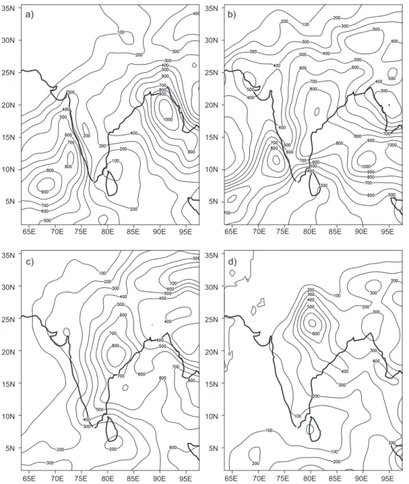
(17) 157. Rainfall analysis using conventional and non-conventional data. 35N. 35N. a). 30N. 30N. 25N. 25N. 20N. 20N. 15N. 15N. 10N. 10N. 5N. 5N. 65E 35N. 70E. 75E. 80E. 85E. 90E. 65E. 95E 35N. c). 30N. 30N. 25N. 25N. 20N. 20N. 15N. 15N. 10N. 10N. 5N. 5N. 65E. 70E. 75E. 80E. 85E. 90E. 95E. b). 70E. 75E. 80E. 85E. 90E. 95E. 70E. 75E. 80E. 85E. 90E. 95E. d). 65E. Fig. 10. Same as Fig. 9 but for model predicted rainfall.. Once the results for 2001 were found encouraging, the merging technique was applied to 2003 data to confirm the usefulness of the technique. The comparison has been made among the analyses of GPCP, CMAP, IMD and merged analysis for the months of June to September 2003. Figures 9 and 10 show the satellite based rainfall and model estimated rainfall, respectively, for the year 2003. For the month of June 2003, the merged analysis (Fig.11d) shows the heavy orographic rainfall about 600 to 800 mm along the west coast of India. IMD analysis (Fig. 11c) also shows heavy rainfall along the west coast. IMD and merged analyses (Fig. 11c, d) show pockets of.

(18) 158. S.G. Narkhedkar et al.. 35N. 35N. a). 30N. 30N. 25N. 25N. 20N. 20N. 15N. 15N. 10N. 10N. 5N. 5N. 65E 35N. 70E. 75E. 80E. 85E. 90E. 65E. 95E 35N. c). 30N. 30N. 25N. 25N. 20N. 20N. 15N. 15N. 10N. 10N. 5N. 5N. 65E. 70E. 75E. 80E. 85E. 90E. 95E. b). 70E. 75E. 80E. 85E. 90E. 95E. 70E. 75E. 80E. 85E. 90E. 95E. d). 65E. Fig. 11. Same as Fig. 4 but for 2003.. heavy rainfall along the north-east India. Along the west coast and also over north-east India the pattern of rainfall from merged analysis (Fig. 11d) was similar to the IMD analysis (Fig. 11c). The corresponding GPCP (Fig. 11a) and CMAP (Fig. 11b) rainfall analyses are not showing the similar pattern of rainfall as IMD analysis. They are showing heavy rainfall contour over the head of the Bay of Bengal which is in contrast to the observed facts (Fig. 11c, IMD analysis). However, CMAP shows slightly higher rainfall than GPCP. Almost similar description can be given about all other months, July, August and September 2003 (Figs. 12, 13 and 14, respectively). Shown in Figure 15.

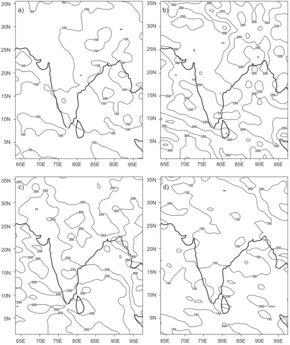
(19) 159. Rainfall analysis using conventional and non-conventional data. 35N. 35N. a). 30N. 30N. 25N. 25N. 20N. 20N. 15N. 15N. 10N. 10N. 5N. 5N. 65E 35N. 70E. 75E. 80E. 85E. 90E. 65E. 95E 35N. c). 30N. 30N. 25N. 25N. 20N. 20N. 15N. 15N. 10N. 10N. 5N. 5N. 65E. 70E. 75E. 80E. 85E. 90E. 95E. b). 70E. 75E. 80E. 85E. 90E. 95E. 70E. 75E. 80E. 85E. 90E. 95E. d). 65E. Fig. 12. Same as Fig. 5 but for 2003.. (a-d) is the total seasonal rainfall for the GPCP, CMAP, IMD and merged analyses of 2003. IMD and merged analyses show total seasonal rainfall along the west coast around 1800 and 2200 mm, respectively. At the foothills of Himalayas and north eastern parts of India high rainfalls (about 1200 to 1600 cm) are seen. Over the same region, total seasonal rainfall shown by GPCP and CMAP are considerably low. Over oceanic region surrounding India, merged analysis could not produce similar features of rainfall analysis as that of CMAP or GPCP. This means that over the oceanic region for the blending.

(20) 160. S.G. Narkhedkar et al.. 35N. 35N. a). 30N. 30N. 25N. 25N. 20N. 20N. 15N. 15N. 10N. 10N. 5N. 5N. 65E 35N. 70E. 75E. 80E. 85E. 90E. 65E. 95E 35N. c). 30N. 30N. 25N. 25N. 20N. 20N. 15N. 15N. 10N. 10N. 5N. 5N. 65E. 70E. 75E. 80E. 85E. 90E. 95E. b). 70E. 75E. 80E. 85E. 90E. 95E. 70E. 75E. 80E. 85E. 90E. 95E. d). 65E. Fig. 13. Same as Fig. 6 but for 2003.. purpose the data should be more reliable and close to the observations. For this reason in the future study TRMM satellite product will be used which has proved it utility. 6. Summary and conclusions In this paper following the algorithm developed by Xie and Arkin (1996) we have constructed monthly rainfall over Indian and adjoining region for two monsoon seasons (2001 and 2003) by.

(21) 161. Rainfall analysis using conventional and non-conventional data. 35N. 35N. a). 30N. 30N. 25N. 25N. 20N. 20N. 15N. 15N. 10N. 10N. 5N. 5N. 65E 35N. 70E. 75E. 80E. 85E. 90E. 65E. 95E 35N. c). 30N. 30N. 25N. 25N. 20N. 20N. 15N. 15N. 10N. 10N. 5N. 5N. 65E. 70E. 75E. 80E. 85E. 90E. 95E. b). 70E. 75E. 80E. 85E. 90E. 95E. 70E. 75E. 80E. 85E. 90E. 95E. d). 65E. Fig. 14. Same as Fig. 7 but for 2003.. merging gauge-based rainfall, INSAT 1-D estimate and numerical weather forecast model predicted rainfall. The merging is done in two steps. In the first step satellite and model estimates are combined linearly based on maximum likelihood estimate method and in the second step the combined analysis is blended with the IMD gauge analysis to produce merged analysis. Results showed substantial improvements in the merged analysis relative to the individual sources in describing the regional precipitation field. The amount of rainfall and its distribution over land match well with the IMD analysis. Merging over land and ocean has been done separately. The characteristics of the merged.

(22) 162. S.G. Narkhedkar et al.. 35N. 35N. a). 30N. 30N. 25N. 25N. 20N. 20N. 15N. 15N. 10N. 10N. 5N. 5N. 65E 35N. 70E. 75E. 80E. 85E. 90E. 65E. 95E 35N. c). 30N. 30N. 25N. 25N. 20N. 20N. 15N. 15N. 10N. 10N. 5N. 5N. 65E. 70E. 75E. 80E. 85E. 90E. 95E. b). 70E. 75E. 80E. 85E. 90E. 95E. 70E. 75E. 80E. 85E. 90E. 95E. d). 65E. Fig. 15. Same as Fig. 8 but for 2003.. analysis have been examined by comparing with the available independent data sets like GPCP and CMAP analyses. This study demonstrates the potential of this merged datasets for monitoring and analysis of monsoon rainfall systems. A comparison with the satellite estimate shows that the merged analysis could take the advantage of land-based rain gauge where the performance of the satellite estimate is poor particularly for orographic rainfall. The magnitude and distribution of orographic rainfall near the west coast of India is very realistic when compared to both the GPCP and CMAP analyses..

(23) Rainfall analysis using conventional and non-conventional data. 163. CMAP is not able to capture orographic rainfall along the foothills of Himalayas. Over land, rain areas and rain shadow areas are clearly demarcated. More work is needed to improve the quality of the individual data sources over tropical oceans. Knowing the limitations of the performance of the NWP model output over tropics, it is planned to use TRMM (Tropical Rainfall Measuring Mission) data expecting that the error structures of the individual sources can be estimated more accurately over oceanic region. As the quality of the merged analysis depends on the accuracy of the input data sources, it is necessary to improve the quality of the individual data sets. It is planned to prepare merged analyses datasets on daily and monthly scale for a longer period. Acknowledgment The authors are grateful to Prof. B. N. Goswami, Director, Indian Institute of Tropical Meteorology, Pune, for his encouragement and providing us with the necessary facilities. Thanks are also due to Head, Forecasting Research Division for his support. We would like to thank all the authors and creators of GPCP and CMAP datasets for providing the monthly total values of rainfall. We are grateful to India Meteorological Department for satellite rainfall estimates from INSAT and objectively analysed rainfall data. The authors wish to thank the anonymous reviewers for their constructive comments. GrADS software used for preparing the diagrams is also thankfully acknowledged. References Adler R. F., A. J. Negri, P. R. Keehn and I. M. Hakkarinen, 1993. Estimation of monthly rainfall over Japan and surrounding waters from a combination of low-orbit microwave and geosynchronous IR data. J. Appl. Meteor. 32, 335-356. Adler R. F., G. J. Huffman and P. R. Keehn, 1994. Global rain estimates from microwave-adjusted geosynchronous IR data. Rem. Sens. Rev. 11, 125-152. Arkin P. A. and B. N. Meisner, 1987. The relationship between large scale convective rainfall and cold cloud over the western hemisphere during 1982-84. Mon. Weather Rev. 115, 51-74. Arkin P. A. and P. Xie, 1994. The global precipitation climatology project: First Algorithm Intercomparison Project. Bull. Amer. Meteor. Soc. 75, 401-419. Arpe K., 1991. The hydrological cycle in the ECMWF short-range forecasts. Dyn. Atmos. Oceans 16, 33-60. Gates W. L., 1992. AMIP: The atmospheric model intercomparision project. Bull. Amer. Meteor. Soc. 73, 1962-1970. Higgins R. W. and W. Shi, 2000. Dominant factors responsible for interannual variability of the Summer monsoon in the Southwestern United States. J. Clim. 13, 759-776. Huffman G. J., R. F. Adler, P. A. Arkin, A. Chang, R. Ferraro, A. Gruber, J. Janowiak, A. McNab, B. Rudolf and U. Schneider, 1997. The Global Precipitation Climatology Project (GPCP) combined precipitation dataset. Bull. Amer. Meteor. Soc. 78, 5-20. Janowiak J. E. and P. A. Arkin, 1991. Rainfall variations in the tropics during 1986-1989. J. Geophys. Res. 96, 3359-3373. Kripalani R. H., S. V. Singh and P. A. Arkin, 1991. Large scale features of rainfall and OLR over India and adjoining regions. Cont. Atmos. Phy. 64, 159-161..

(24) 164. S.G. Narkhedkar et al.. Mitra A. K., M. Das Gupta, S. V. Singh and T. N. Krishnamurti, 2003. Daily rainfall for the Indian monsoon region from merged satellite and rain gauge values: large scale analysis from the real-time data. J. Hydrometeorol. 4, 769-781. Narkhedkar S. G., S. K. Sinha and A. K. Mitra, 2008. Mesoscale objective analysis of daily rainfall with satellite and conventional data over Indian summer monsoon region. Geofizika 25, 159-178. Rajeevan M., J. Bhate, J. D. Kale and B. Lal, 2006. High resolution daily gridded rainfall data for the Indian region: Analysis of break and active monsoon spells. Curr. Sci. 91, 296-306. Reynolds R. W., 1988. A real-time global sea surface temperature analysis. J. Climate 1, 75-86. Roy Bhowmik S. K. and A. K. Das, 2007. Rainfall analysis for Indian monsoon region using the merged rain gauge observations and satellite estimates: evaluation of monsoon rainfall features. J. Earth. Sys. Sci. 116, 187-198. Shepard D., 1968. A two dimensional interpolation function for irregularly spaced data. 23rd National Conference of American Computing Machinery, Princeton, N J, ACM, 517-524. Shi W., R. W. Higgins, E. Yarosh and V. E. Kousky, 2001. The annual cycle and variability of precipitation in Brazil. NCEP/Climate Prediction Center Atlas. No. 9, NOAA, NWS. Silva V. B. S., V. E. Kousky, W. Shi and R. W. Higgins, 2007. An improved gridded historical daily precipitation analysis for Brazil. J. Hydrometeorol. 8, 847-861. Sinha S. K. and S. G. Narkhedkar, 2006. Barnes objective analysis scheme of daily rainfall over Maharashtra (India) on a mesoscale grid. Atmósfera 19, 109-126. WMO,1993. Global observations, analyses and simulation of precipitation. World Climate Research Programme. Rep. WCRP-78, WMO/TD 544, World Meteor. Org., Geneva, 136 pp. Xie P. and P. A. Arkin, 1995. An intercomparison of gauge observations and satellite estimates of monthly precipitation. J. Appl. Meteor. 34, 1143-1160. Xie P. and P. A. Arkin, 1996. Analyses of global monthly precipitation using gauge observations, satellite estimates and numerical model predictions. J. Climate 9, 840-858. Xie P. and P. A. Arkin, 1997. Global precipitation: A 17-year monthly analysis based on gauge observations, satellite estimates and numerical model outputs. Bull. Amer. Meteor. Soc. 78, 2539-2558. Xie P., J. E. Janowiak, P. A. Arkin, R. Adler, A. Gruber, R. Ferraro, G. J. Huffman and S. Curtis, 2003. GPCP pentad precipitation analyses: An experimental dataset based on gauge observations and satellite estimates. J. Climate 16, 2197-2214. Xie P., A. Yatagai, M. Chen, T. Hayasaka, Y. Fukushima, C. Liu and S. Yang S., 2007. A gaugebased analysis of daily precipitation over East Asia. J. Hydrometeorol. 8, 607-626..

(25)

No results found