Processing of kinetic microarray signals

Sensors and Actuators B 128 (2007) 75–82

Processing of kinetic microarray signals

Thomas Braun

, Franc¸ois Huber, Murali Krishna Ghatkesar, Natalija Backmann,

Hans Peter Lang, Christoph Gerber, Martin Hegner

National Center of Competence for Research in Nanoscience, Institute of Physics, University of Basel, 4056 Basel, Switzerland

Received 13 February 2007; received in revised form 25 May 2007; accepted 25 May 2007 Available online 29 May 2007

Abstract

Measurement of kinetics using microarrays requires adapted experimental analysis for data evaluation and normalization. Here we present a new algorithm based on alignment of data, which solves inconsistencies of current normalization methods utilizing baseline correction. Our results show that this method leads to better data consistency and relative errors four times smaller on average.

© 2007 Elsevier B.V. All rights reserved.

PACS: 07.05.Kf; 68.43.Mn; 07.07.Df; 87.90.+a

Keywords: Microarray; Kinetic; Time resolved; Baseline correction; Sensor; Cantilever; Algorithm; Curve alignment

1. Introduction

Microarray techniques are of indisputable value for today’s genomic and proteomic research in biology and medicine. Traditionally, these methods do not directly provide kinetic information. In recent years, modern microarray technologies evolved which will enable the researcher to design new kinds of experiments involving time-resolved measurements. Such techniques include surface plasmon resonance imaging [1], ellipsometry[2], surface acoustic wave sensors[3], nano-wire based[4]and cantilever-based methods[5].

Data processing plays an important role in the interpreta-tion of time-resolved data from microarray measurements. Since these signals are based on extremely small sensor areas (in the

␮m2range) relatively large variations may occur during func-tionalization with probe molecules and detection of the signal upon binding of an analyte. This leads eventually to large rel-ative errors in the data compared to signals from sensors with large signal-integration areas. To get an estimate of data quality, measurements are performed in redundancy with several sensors functionalized in the same way. These different channels (pos-itive and negative controls) are then averaged. In general the average of the references (negative control) is subtracted from

∗_{Corresponding author.}

E-mail address:[email protected](T. Braun).

the average of positive controls to remove contributions from unspecific interactions (differential signal).

However, averaging of multiple signals is problematic for kinetic data: before averaging, the data must be corrected for dif-ferent offsets and drifts. Traditionally this is done by a baseline correction whereby an initial measurement period is analyzed in the absence of an analyte. The signal recorded during this initial period is fitted by a linear baseline, which is then extrap-olated and subtracted from the raw measurement curve. Such a procedure evokes several problems, which are not observed in measurements involving only one reference and one positive sig-nal. (a) The initial linear fit is prone to errors due to noise. These errors are amplified when extrapolated to the complete duration of the measurement. (b) Linear progression of drift might be an unjustified assumption. If only one negative and one positive signal are recorded, the reference may be simply subtracted.

Therefore it is reasonable to assume that the relative error of the average will increase over time. This is in contradiction to the theory that real measurements can be interpreted as ideal measurements plus noise. In this case the relative error would be constant.

Normalization of microarray data is a significant problem, which needs to be solved to be able to compare data from different experiments and correct for local variations of the indi-vidual sensors. In the case of nanomechanical microarrays the mechanical response of individual sensors can be tested prior to a (biological) experiment by a heat test[6,7].

0925-4005/$ – see front matter © 2007 Elsevier B.V. All rights reserved. doi:10.1016/j.snb.2007.05.031

The use of baseline correction methods may increase the errors due to inaccurate offsets as opposed to the normaliza-tion test done before. Here we propose an alignment-based method that utilizes additional normalization factors prevent-ing such errors and leadprevent-ing to optimal data extraction in kinetic microarray experiments. In short, this alignment procedure shifts and rotates the curves for optimal overlapping of all data-sets in magnitude and time as well as in a rotation angle for the complete duration of the experiment. Additionally a factor scal-ing the data in magnitude is introduced which is responsible for the normalization. Here we use a normalization coefficient derived from the heat test to demonstrate the normalization routine.

In the following, we shall use a test data-set acquired in a standard static nanomechanical cantilever experiment (pH mea-surement, similar experiments are discussed in detail in Ref. [8]) to compare the effects of baseline correction and align-ment methods for the processing of cantilever-based microarray sensor data.

2. Materials and methods 2.1. Reagents

Na2HPO4, NaH2PO4, NaCl, hexadecane-1-thiol (HDT), 16-mercapto-hexa-decanoic-1-acid (MHA), HPLC-grade water and ethanol were all purchased from Fluka (Buchs, Switzerland). MHA and HDT were dissolved in ethanol to a final concentra-tion of 4 mM each. Two different pH soluconcentra-tions were prepared for the experiments: NaH2PO4was dissolved in water to a final concentration of 100 mM resulting in a pH of 4.3 (low-pH solu-tion). Na2HPO4was dissolved in water to a final concentration of 100 mM resulting in a pH of 8.6 (high-pH solution). Both solutions were adjusted to 300 mM in ionic strength using 1 M NaCl.

2.2. Cantilever preparation

Microfabricated arrays with eight identical silicon cantilevers at a pitch of 250␮m, a length of 500␮m, a width of 100␮m and a thickness of 1␮m (spring constant of 0.0025 N/m) were provided by the Micro- and Nanomechanics group at the IBM Zurich Research Laboratory. The cantilevers were prepared as described in detail elsewhere[9,10]. Briefly, the cantilever arrays were cleaned in Piranha solution and then coated on their upper side with 2 nm of Ti (99.99%, JohnsonMatthey), followed by 20 nm of Au (99.999%, Goodfellow), using an Edwards L400 e-beam evaporator operated at a base pressure below 10−6mbar and evaporation rates of 0.07 nm/s. Afterwards, the cantilever array was functionalized using eight micro-capillaries (inner diameter 150␮m; from Garner Glass, Claremont, CA), one for each cantilever, filled with either MHA or HDT solution, thereby activating the two groups of four cantilevers either with a pH sensing layer (MHA) or a reference layer (HDT). After 20 min, the functionalized cantilever array was washed twice in low-pH solution.

2.3. pH experiment

The functionalized cantilever array was inserted into a liquid chamber (volume: 50␮l) and mounted at an angle of 11◦with respect to the incident laser beam (time-multiplexed vertical-cavity surface-emitting laser; wavelength 760 nm, Avalon Photonics, Zurich, Switzerland). The laser beam was redirected by a mirror to a PSD (position-sensitive detector, SiTek, Partille, Sweden). Data were acquired using a multifunctional data-acquisition board (National Instruments, Austin, TX) driven by LabView software. The software also controlled the liquid-handling system of the setup, the syringe pump (GENIE, Kent Scientific Corp., Torrington, CT), and a 10-position valve sys-tem (Rheodyne, Rohnert Park, CA). The entire setup was placed inside a temperature-controlled box (Intertronic; Interdiscount, Switzerland), which was equilibrated to 23◦C. The cantilevers were equilibrated in low-pH solution before and after each injec-tion of high-pH soluinjec-tion. Three pulses of high-pH soluinjec-tion were conducted. In the first injection, 200␮l high-pH solu-tion was injected at a flow rate of 20␮l/min (section II of Fig. 3A–D). Subsequently, the cantilevers were equilibrated with an injection of 200␮l low-pH solution at a flow rate of 20␮l/min. The following two pH changes (sections IV and V, VI and VII) were performed under a constant flow rate of 20␮l/min while switching from one pH solution to the other.

2.4. Data processing

All data-processing algorithms were implemented in the IGOR pro data analyze environment (www.wavemetrics.com). The operations were implemented in a framework of a cantilever-sensor processing tool called NOSEtools [11,6] (http://web.mac.com/brunobraun/iWeb/NOSETools/). For de-tails see Section3.1.

3. Results

As a test system we measured the pH-dependent detection of eight cantilevers in one microarray. Individual cantilevers were functionalized either with 16-mercapto-hexadecanoic-1-acid (MHA, cantilevers 5–8) as pH sensing cantilevers or with hexadecane-1-thiol (HDT, cantilevers 1–4) as references. To run the test we used a cantilever array with known large mechanical variations among the individual cantilevers for testing purpose. Standard experiments are usually not performed with such inho-mogeneous arrays.

One of the advantages of nanomechanical cantilever sensors is the option to perform a normalization test prior to the experi-ment. This test allows to assess the mechanical homogeneity of the cantilevers in the array by performing a heat test: the mea-surement chamber containing the cantilever array was heated (by 2◦C for 30 s) and allowed to cool again to the working tem-perature. The asymmetric gold coating (see Section2) forced compressive bending of the cantilevers due to the different ther-mal expansion coefficients of gold, titanium and silicon. These heat tests are in general highly reproducible.

These data were used to normalize the pH-experiment which was performed directly after the heat test. During this part of the experiment, two different buffers with a different pH (but iden-tical ionic strength) were injected in sequence for three pulses (see Section2for details).

All data analysis steps were performed in two different ways: first with baseline correction and normalization as described before[6]and second by aligning and normalization of the data (see next Section).

3.1. Alignment algorithm

The alignment of the data was done by pairwise alignment of one curve on a reference. The program minimized the distance of the transformed data pointy(x) =E(y(x+x)) +y+ sin(α)x (withxthe shifting in the time axis,ya constant offset and

αthe rotation angle,Eis an expansion/compression coefficient used for data normalization) to the reference data pointyref(x) using a standard Levenberg–Marquardt algorithm[12].

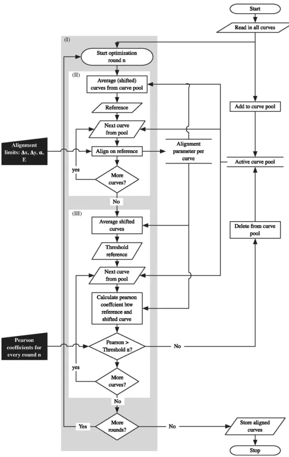
The alignment-reference for the first round was obtained by averaging all original raw data-sets. In this way the influence of a single raw curve on the alignment result is minimized (pseudo reference-free alignment). The alignment was performed in several rounds. After every round a new reference of the shifted and rotated curves was calculated, and in the next round the original data-sets were aligned on the new reference again (seeFig. 1). At the end of an optimization round, the aligned curves were compared to the reference and a cross-correlation (Pearson) coefficient reflecting the similarities between the curves was calculated. The alignment improved with the num-ber of performed rounds. This was reflected in the calculated cross-correlation coefficients asymptotically approaching an upper limit (data not shown).

The operator can influence the alignment algorithm with boundary conditions (black boxes in Fig. 1). First, limits for the shifts (x,y) and for the maximal rotation angleαcan be given. If expansion is allowed, a maximal expansion or com-pression factorEcan be set. Second, a list with increasing cross-correlation coefficients for every round can be created. Curves which revealed a lower cross-correlation coefficient than a given threshold in a specific round were removed from the active curve pool. This was never the case in all alignment operations performed on the experimental data used for this publication.

The factorEwas introduced for normalization of the data. Using a normalized reference to align the heat test data, the normalization coefficients were determined prior to the analysis of the pH experiment. The normalization factors determined were carried over to the real experiment and kept constant for these alignments (see next Section).

Note that a constant normalization factorEdid not change signals relative to each other in all our tests (seeSupplemental material, Section 1).

3.2. Analysis of heat test

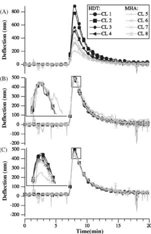
Results of the heat test are presented inFig. 2. Panel A depicts the baseline corrected data. These data were obtained by

sub-tracting an extrapolated baseline (between 0 min and 6.5 min) to remove offsets and drifts. The different magnitudes of can-tilever responses reflect the different nanomechanical properties of the individual cantilevers and are not due to varying laser posi-tions on the cantilever as visually monitored by a CCD camera. The peak heights obtained for this cantilever array varied from roughly 200 nm up to more than 800 nm. This is atypical for standard cantilever arrays but useful to evaluate the proposed data analysis routine.

Fig. 2, panel B shows the normalized heat-test data which was calculated as follows: from the baseline-corrected data a peak search was performed. In a second step all data were divided with the individual peak heights of the cantilevers and multiplied with the average peak height of all cantilevers. This factor was later used for the normalization of the subsequent pH experiment.

For comparison, the heat-test data was aligned as described in Section 3.1(seeFig. 2panel C). To find the normalization coefficients, the reference was always normalized with its peak height and multiplied with the averaged peak heights of the base-line corrected data. This allows for a direct comparison of the two results. The determined normalization coefficients were car-ried over to the pH experiment. The average of the normalization coefficient was found to be 1.1. Time shifts were negligibly small (maximally 1.2 s, which has to be compared to the time for the multiplexed readout of all eight cantilevers of 2.9 s).

3.3. Analysis of pH experiment

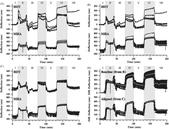
The pH experiment was performed by sequential injection of two buffers of different pH but equal ionic strength. InFig. 3A–D the time span where the low-pH buffer is flowed through is indi-cated with a white and the time periods with high-pH solution are marked with a gray background.

3.3.1. Baseline correction and normalization

To compare the alignment with the baseline-correction method, the start sequence of the raw data (section I inFig. 3) was fitted with a linear model between 0 min and 10 min. The baseline was extrapolated to the whole duration of the measure-ment and subtracted from the raw data. The result is depicted inFig. 3A. In a second step, the data-set was divided with the normalization factors obtained from the heat test as described in Section3.2. The normalized data are displayed inFig. 3B. 3.3.2. Alignment of pH experiment data

To ensure a better comparison between the two processing methods, we used the initially baseline corrected data depicted inFig. 3A as input data-sets. The reference for the first alignment round was obtained by averaging these input data. The alignment was performed using the constant normalization coefficients from the heat-test data alignment. This stretches or compacts the raw data during alignment which corresponds to the nor-malization of the baseline correction approach. This process is independent from initial offsets and additional baselines (see Supplemental material, Section 1).Fig. 3C shows the result of the alignment.

Fig. 1. Alignment algorithm utilizing the average of the input curves as start reference. The alignment was optimized in several rounds (box I). The optimization was performed for every round in two steps. First, the raw curves were aligned to the reference (box II). Second a new reference based on the shifted and rotated curves was created. A cross-correlation coefficient (Pearson) was calculated between every curve and the new reference. Curves with correlation coefficients below a threshold were deleted from the active curve pool (box III). At the beginning of every optimization round, a new reference from the shifted and active curves was calculated.

Fig. 2. Analysis of the heat test. MHA functionalized cantilevers (pH sensitized) are depicted in gray, HDT coated ones (pH insensitive) with black lines. (A) baseline corrected raw data, (B) normalized data after baseline correction, (C) alignment of baseline corrected raw data with adjustable normalization factors. Insets in panel (B) and panel (C): peak region at higher magnification, also indicated by a box in the main graph. The markers (every fourth data point) indicate the cantilever (CL) number (legend).

3.3.3. Differential signal

The aligned and normalized data-sets were averaged and the corresponding standard errors calculated. The HDT average was subtracted from the MHA average and the error prop-agation estimated. The results are shown in Fig. 3D. The global-mean standard-error for the aligned data was 11.4 nm (upper curve) and for the baseline corrected data 46.8 nm (lower curve).

The relative errors of the differential signal at high pH 8.6 (sections II, IV, and VI inFig. 3) were calculated and are sum-marized inTable 1. On average, the relative error of the pH measurements was four times lower if the curves were aligned in contrast to baseline corrected data analysis.

Table 1

Relative errors of the differential signal for high-pH solution (differential nanomechanical response of pH sensitized cantilevers to jumps of 4.3 pH units)

Section

I IV VI

Baseline corrected 8.7% 11.9% 17.5%

Aligned 3.2% 3.3% 2.8%

The section numbers correspond to the sections inFig. 3.

All the calculations were also performed with the raw data without normalization (baseline correction as shown inFig. 3, aligning with normalization factors E= 1; see Supplemental material, Section 2). Comparing the averages of the aligned and baseline-corrected data revealed that the aligned data resulted in better data consistency and standard errors. However, the cal-culation of the differential signal (MHA data minus HDT data) for the not-normalized averages did not show significant fea-tures, neither for aligned nor for the baseline corrected data (see Section4).

4. Discussion

Comparison of data evaluation via baseline-correction with the alignment-based approach revealed that the latter yielded more precise results (in average four times smaller relative errors, seeTable 1). This finding is of outmost importance to interpret data only slightly above noise level and can massively enhance evaluation of experiments at the sensitivity limit of kinetic microarray devices.

We have chosen a test data-set with several challenges to push data processing to its limits: large variations of individ-ual nanomechanical properties and large noise level in one of the cantilever responses due to instabilities in the vertical-cavity surface-emitting laser operation (cantilever No. 5,Fig. 2). Further the positively functionalized cantilevers (MHA) show systematically lower heat-peak deflections as the negative ones (HDT, see Fig. 2A) due to different cantilever stiffness. This is never observed in this extent with standard quality cantilever arrays. Therefore, data evaluation without correction of differing mechanical properties through normalization led to a differen-tial signal with insignificant deflection changes upon pH change (Supplemental material, Section 2). The heat test represents a pre-calibration of the response of the mechanical signal trans-ducer. Such a test would relate to a chemical activation analysis used in other microarray technologies prior to the experimental exposure to (bio)-analytes. Such a pre-calibration is not possible with traditional microarray technologies and represents one of the advantages of nanomechanical sensing arrays.

The applied alignment algorithm is fast, reproducible and reliable. Moreover it is simple to use. It is only possible to influence the outcome by changing the shifting, rotation or nor-malization factor limits. In all our alignment tests the applied limits never changed the outcome of the alignment or the analysis of the experiment, as long as they were set wide enough. Further-more, the choice of more stringent cross-correlation coefficients allows to set objective criteria for data exclusion from defective sensors in very large arrays. Optionally the alignment algorithm allows to shift data in time. The observed time shifts were always below the spacing in time of data points due to the multiplexed readout of the individual sensors. This optional time shift could be of great value for the data analysis of large sensor arrays with long distances for the ligands to diffuse to the binding sites. In this case, the positive and negative control average also must be synchronized by alignment. In the analysis here time shifts were allowed but only negligible shifts were observed of max-imally 2.9 s. This option did not change the final outcome at

Fig. 3. Normalization and averaging of the pH-experiment. Injection periods with high-pH buffer are indicated with gray boxes, while low-pH buffer periods with white background. (A) baseline corrected raw data without normalization, and the starting point of all subsequent calculations, (B) conventional normalized data (the baseline corrected data from (A) were divided by the normalization factor derived from the heat test), (C) alignment and normalization by the new algorithm (the normalization factors were derived from heat test analysis), (D) differential signal of averaged aligned and baseline corrected data-sets (MHA−HDT). The error bars indicate the propagated standard errors of the averages. Note that for panels (A–C) the axis labels for the HDT data only comprise half the span of the MHA data to facilitate the interpretation. The markers label every 100th data point. Markers in panels (A–C) are identical withFig. 2; in panel (D) the data points are marked by white circles.

all and these tiny time shifts are not the reason for the large improvement of the standard and relative errors as compared to baseline-corrected data (seeFig. 3andTable 1).

In the first step, the heat-test data-set was analyzed to get the normalization coefficients for both methods (the baseline correc-tion approach and the analysis by alignment). These coefficients were later used to correct the pH data for mechanical inhomo-geneities between the cantilevers. The analysis of the heat test (Fig. 2) shows clearly that with the alignment procedure the full characteristics of the Peltier peak are taken into account (panel C). This finding is in contrast to the baseline corrected normal-ization procedure, where determination of the peak height in the heat test is prone to be affected by local noise at the peak region as seen in the insets of Fig. 2. This is obvious with cantilever 5 (marker +), where the detection method is running into the nonlinear region of the PSD and is therefore stretched too much during normalization by the baseline-correction approach (see panel B). In the case of aligning the data (panel C), cantilever 5 does not reach the peak and is flattened, but the rest of the

curve is properly aligned to the ensemble of the heat test data. A typical finding is also the large curve spread in the end of the short measurement which is not observed for aligned data. Note that the reference for alignment of the heat-test data was normalized. To do this, the initial input data was baseline cor-rected and normalized. For the subsequent optimization rounds no baseline correction was needed.

In the second step, the pH experiment was analyzed and again the two methods (baseline correction versus alignment) were compared. The data-sets were normalized by the corresponding methods with the coefficients found during the heat peak anal-ysis. An analogue analysis without normalization is presented insupporting materials (Section 2). The comparison of panel A (baseline corrected data-set) and panel B (baseline corrected and normalized data-set) inFig. 3reveals that the deviation of the curve drift is improved only marginally by the normaliza-tion. For some cantilevers the spread even increased. This is not only due to errors during determination of the normaliza-tion factors in the heat test as discussed above, but also caused

by the erroneous offsets increasing with time introduced by the initial baseline correction of the pH data. The latter is due to the errors during baseline characterization in the beginning of the experiment, which are amplified over time. The proposed normalization/alignment algorithm is independent from such offsets and baseline corrections. This is visible inFig. 3C, where the overlap of curves is massively improved (compare with panel A). The alignment based normalization of the pH data also decreased the measurement errors as compared to the aligning of raw data without normalization.

Note that these normalization coefficients must be derived from tests depending on the nature of the used sensor or trans-ducer, respectively, but the proposed algorithm is independent of the used measurement method and normalization criteria.

The alignment is only slightly affected by the large noise level as observed in the response of cantilever 5 inFigs. 2 and 3. Note that such noise influenced baseline correction substantially due to introduction of large errors for the initial baseline deter-mination; these are further amplified over time during baseline extrapolation.

In the final operation, the differential signal between the pH sensitive cantilevers (MHA functionalized) and reference cantilevers (HDT functionalized) for both methods (base-line correction and alignment) was calculated. For this, the corresponding signals were averaged and the reference was subtracted. The found result is in excellent agreement with previously published measurements[9]. The differential signal (Fig. 3D) for aligned and baseline-corrected data reveals that the main difference between evaluation methods is not the qualita-tive development of the differential signal, but mainly the much higher data quality, which is clearly demonstrated in regard to the error bars representing the propagated standard error.Table 1 also clearly shows that the relative error of the differential signal in baseline-corrected data-analysis increases over time as postu-lated in Section1. This is not the case for the differential signal deduced from the aligned data. This will also allow to evaluate correctly long-term experiments showing signals at the resolu-tion limit of the instrument. The four times lower relative error for the aligned data signals allows to reach higher resolution and sensitivities with the same instrument or equal data qual-ity with less sensor response statistics. Please also note that the pH “insensitive” HDT cantilever also undergoes nanomechani-cal deflection changes upon injection of different pH solutions. This is induced by chemical reactions on the non-functionalized silicon surface (for details see[8]).

The proposed algorithm based on alignment is free from the assumption of baseline propagation. With constant normal-ization coefficientsE= 1 and provided that time-shifts are not allowed, the method represents an optimal way of finding the baseline for all curves before averaging. This avoids the pitfalls for baseline correction described above. Normalization changes data scaling by definition. In all our tests the normalization algo-rithm used here did not change signals relative to each other. This finding was independent of the baseline of the curve, e.g. the outcome of the heat-test data alignment was independent, whether the input data were baseline corrected before or not (seeSupplemental material, Section 1).

The test data used here posed several hurdles for subsequent data processing which were successfully overcome. In addition, processing of standard data-sets from DNA hybridization and protein detection experiments confirmed the finding that the alignment/normalization algorithm proposed here improves the quality of the results in general (data not shown).

5. Conclusions

The alignment of kinetic microarray data resulted in four times smaller relative errors for the measurements than evaluated by baseline-correction. This improvement will facilitate exper-imental design and data interpretation close to the resolution limit of the measurement instrument.

Acknowledgments

We thank Olivia Keiser (Institute for Social and Preven-tive Medicine, University of Bern) for carefully reading and commenting the manuscript. Financial and general support is acknowledged from SNF (NCCR nanoscale science), the Cleven-Becker Stiftung, Endress Foundation and the ELTEM Regio.

Appendix A. Supplementary data

Supplementary data associated with this article can be found, in the online version, atdoi:10.1016/j.snb.2007.05.031. References

[1] C. Jordan, R. Corn, Surface plasmon resonance imaging measurements of electrostatic biopolymer adsorption onto chemically modified gold sur-faces, Anal. Chem. 69 (1997) 1449–1456.

[2] Z.H. Wang, G. Jin, A label-free multisensing immunosensor based on imaging ellipsometry, Anal. Chem. 75 (2003) 6119–6123.

[3] T.M.A. Gronewold, A. Baumgartner, E. Quandt, M. Famulok, Discrimi-nation of single mutations in cancer-related gene fragments with a surface acoustic wave sensor, Anal. Chem. 78 (2006) 4865–4871.

[4] Y. Cui, Q. Wei, H. Park, C.M. Lieber, Nanowire nanosensors for highly sensitive and selective detection of biological and chemical species, Science 293 (2001) 1289–1292.

[5] H.P. Lang, M. Hegner, C. Gerber, Nanomechanical cantilever array sen-sors, in: Springer Handbook of Nanotechnology, 2nd ed., Springer Verlag, Berlin, 2006, 443–450.

[6] T. Braun, N. Backmann, A. Bietsch, C. Gerber, H.-P. Lang, M. Hegner, Conformational change of bacteriorhodopsin quantitatively monitored by microcantilever sensors, Biophys. J. 90 (2006) 2970–2977.

[7] J. Zhang, H.P. Lang, F. Huber, A. Bietsch, W. Grange, U. Certa, R. Mckendry, H.J. Guntherodt, M. Hegner, C. Gerber, Rapid and label-free nanomechanical detection of biomarker transcripts in human RNA, Nat. Nano. 1 (2006) 214–220.

[8] M. Watari, J. Galbraith, H.-P. Lang, M. Sousa, M. Hegner, C. Gerber, M. Horton, R. McKendry, Investigating the molecular mechanisms of in-plane mechanochemistry on cantilever arrays, J. Am. Chem. Soc. 129 (2007) 601–609.

[9] J. Fritz, M.K. Baller, H.P. Lang, T. Strunz, E. Meyer, H.J. G¨untherodt, E. Delamarche, C. Gerber, J.K. Gimzewski, Stress at the solid–liquid interface of self-assembled monolayers on gold investigated with a nanomechanical sensor, Langmuir 16 (2000) 9694–9696.

[10] R. McKendry, J. Zhang, Y. Arntz, T. Strunz, M. Hegner, H.P. Lang, M.K. Baller, U. Certa, E. Meyer, H.-J. Guntherodt, C. Gerber,

Multi-ple label-free biodetection and quantitative DNA-binding assays on a nanomechanical cantilever array, Proc. Natl. Acad. Sci. 99 (2002) 9783– 9788.

[11] T. Braun, M.K. Ghatkesar, V. Barwich, N.B.F. Huber, W.G. An Natlia Nugaeva, H.P. Lang, J.P. Ramseyer, C. Gerber, M. Hegner, Digital pro-cessing of multi-mode nano-mechanical cantilever data, J. Phys. Conf. Ser. 61 (2007) 341–345.

[12] B. Flannery, S. Teukolsky, W. Vetterling, Numerical Recipes in C, Cam-bridge University Press, 1988.

Biographies

Thomas Braunreceived his MS in biophysical chemistry in 1998, and his PhD 2002 in biophysics from the Biozentrum, University of Basel (Switzerland). His thesis was in the field of membrane protein biochemistry, high resolution electron microscopy and digital image processing. As post-doc, he works on the development of kinetic microarray techniques with focus on nanomechanical sensors for membrane protein research and multimode measurements at the Institute of Physics, University Basel.

Franc¸ois Huberreceived his diploma in microbiology from the Biozentrum of the University of Basel, Switzerland in 1989, and a PhD degree in biochemistry from the Institute of Biochemistry of the University of Bern, Switzerland in 1996. In 1996 he joined the group of Prof. Dr. David Boettiger of the University of Pennsylvania, Philadelphia, USA, as a postdoctoral fellow, working on cell adhesion. In 2001 he joined the group of Prof. Dr. Matthias Chiquet at the M.E. M¨uller Institute of the University of Bern, working on mechanical properties of cells. Currently he is working on micro cantilever-based biosensors at the University of Basel in the institute of physics. His research interests are in DNA and protein based micro cantilever biosensors.

Murali Krishna Ghatkesarreceived his MSc degree in Electronics from Uni-versity of Hyderabad, India, and the MSc (Eng) degree in 2001 from Indian Institute of Science, India, for his work on tactile sensors. In 2001, he joined industry and implemented speech codecs on digital signal processors. He went back to Indian Institute of Science in 2003 to work on the development of thin film heat transfer gauges on high enthalpy aerodynamic structures in hyper-sonic shock tunnel. Currently he is pursuing PhD on vibrating microcantilever array in liquid for biosensing applications at Institute of Physics, University of

Basel, Switzerland. His research interest is in the areas of nanobiotechnology, microelectromechanical systems and biophysics.

Natalija Backmannreceived her diploma in chemistry from Moscow State University, Moscow in 1991 and a PhD degree from Free University of Berlin (Faculty of Biology, Chemistry and Pharmacology), Germany in 1999. In 1998–2002, she worked as a research scientist at Institute of Molecular Biol-ogy and BiotechnolBiol-ogy (Free University of Brussels, Belgium) on engineered antibody fragments. Currently she works as a research scientist at University of Basel, Switzerland (Institute of Physics). Her main research interests include development of cantilever-based sensors for detection of proteins, immobiliza-tion of funcimmobiliza-tional proteins on sensor surface and applicaimmobiliza-tion of recombinant antibody fragments and antibody-like molecules.

Hans Peter Langreceived his PhD in physics from the University of Basel in 1994 with a thesis on Scanning tunneling microscopy on high temperature superconductors and carbon allotropes. As a post-doc, he directed research in the pulsed laser deposition and low temperature scanning tunneling microscopy groups at the Institute of Physics in Basel. Since 1996, he is working as a research associate at the IBM Zurich Research Laboratory in the field of cantilever array sensors. Since 2000, he is a project leader focused on biochemical applications of microcantilever array sensors.

Christoph Gerberis the director for Scientific Communication of the NCCR (National Center of Competence for Nanoscale Science) at the Institute of Physics, University of Basel, Switzerland and was formerly a Research Staff Member in Nanoscale Science at the IBM Research Laboratory in R¨uschlikon, Switzerland. For the past 25 years, his research has been focused on nanoscale science. His current interests are biochemical sensors based on AFM tech-nology, chemical surface identification on the nanometer scale with AFM, nanomechanics, nanorobotics, AFM research on insulators, single spin magnetic resonance force microscopy (MRFM) and self-organization and self-assembly at the nanometer scale.

Martin Hegnerreceived his MS Life Science 1989, Swiss Federal Institute of Technology, Biochemistry and his PhD Life Science 1994, Swiss Federal Institute of Technology. In 2006 he was awarded Endress professor for sensors in biotechnology at the University Basel. His primary interests are related to the field of Nanobiology, investiagting molecular interactions by optical tweezers and the development of biosensors based on nanomechanical cantilevers working at the institute for physics in Basel, Switzerland.