447
COMMENT AND DEBATE
Population sampling in longitudinal surveys
Harvey Goldstein
University College London and University of Bristol, UKPeter Lynn
University of Essex, UKGraciela Muniz-Terrera
University of Edinburgh, UKRebecca Hardy
University College London, UKColm O’Muircheartaigh
University of Chicago, USChris Skinner
London School of Economics, UKRisto Lehtonen
University of Helsinki, Finlandhttp://dx.doi.org/10.14301/llcs.v6i4.345
When and why do we need population representative samples?
Harvey Goldstein
University College London and University of Bristol, UK(Received February 2015 Revised April 2015)
Abstract
The paper questions the need for observational studies to achieve representativeness for real populations, in particular for longitudinal studies. It draws upon recent debates and argues for the need to distinguish scientific inference from population inference.
Keywords
Observational studies, longitudinal, representativeness.
Introduction
In a recent issue of the International Journal of Epidemiology (2013, vol 42, 1012-1028)there was a debate about whether analysts have overrated, in epidemiology and social and medical science more generally, the importance of having representative samples from well-defined ‘real’ populations. In this paper the arguments are summarised and developed to understand how they might affect, in particular, longitudinal studies.
Setting out the arguments
The lead paper in this collection by Rothman, Gallacher and Hatch (2013a) argues that efforts to
448
varying relationships. Thus, for example, replication across different ethnic groups, need not involve representative samples from a population containing such groups, but rather ensuring that data are representative of the groups in question and not subject, for example, to selection bias. They suggest that traditional emphasis on statistical significance and obtaining population-unbiased estimates downplays the importance of the scientific need for generalisation and replication. As an example they talk about sampling equal numbers in age groups rather than attempting to match the distribution to the distribution within a population. This particular argument, however, seems weak since, in fact, like the example of ethnic groups, this can be regarded simply as a stratified population sample which, combined with suitable weights, can also be used to make population inferences. They also appear to be concerned largely with the situation where there are pre-existing hypotheses or comparisons of interest, whereas in reality populations are often representatively sampled in order to allow exploratory analyses that rely on sufficient diversity and heterogeneity within the population.They also seek to make a clear distinction between descriptive statistics that require representative samples and analytical statistics that attempt to address scientific hypotheses. In fact, this distinction is often far from clear and I shall return to this point later where I also discuss what exactly is meant by a ‘population’.
Four sets of authors provide responses to Rothman’s paper, three of whom are broadly supportive (Elwood; Nohr & Gleen; Richiardi, Pizzi & Pearce, 2013). I shall deal with these first, then look at the paper (Ebrahim & Davey-Smith, 2013) that takes a somewhat different view and then refer to a rebuttal by Rothman and colleagues (2013b). Elwood (2013) makes the point that that any real population is a historical entity, and when inferences about it are available it may have changed in important ways. Of course, for enumeration purposes, this may still be the best information available. For scientific purposes, however, the real population serves as an instance of an underlying process that generates a data set at a particular time, and where inference is to all possible instances. This is often referred to as a superpopulation approach and the actual real population is treated as if it were a sample from
such a conceptually infinite population. Thus, the actual population serves as a useful data set for exploratory purposes or to test hypotheses within a heterogeneous sample.
All these three respondents point to the importance of taking account of possible confounders and see this as a key concern for scientific purposes. There is some discussion about choosing unrepresentative samples with a high response rate as being preferable to choosing representative samples with a low response rate. The idea of a purposive sample that can achieve a high response rate is an interesting one, but its success depends crucially on knowing the relevant characteristics of the sample. Examples where this might be the case are the use of internet-based surveys and in some cases of clinical trials. In longitudinal studies it is similar to the way in which attrition may be handled. Such studies often settle down to having a fairly stable sample that has a high response rate in repeated waves. Because the initial sample is often fairly representative the characteristics of these initial respondents can be used to ‘adjust’ subsequent analyses to avoid attrition biases.
449
and doesn’t add anything new. They also discuss the meaning of the statistical term ‘bias’ and the importance of being clear what this refers to. This is an important issue and I will return to it below.Defining populations
It is pertinent to ask what is meant by the term ‘population’ and the associated issue of what is meant by ‘bias’. From a statistical viewpoint these are technical terms. Statistical analysis aims to provide estimates for a collection of units (people, institutions etc.) that, at least notionally, can be resampled. Any particular sample is regarded (perhaps conditional on particular variable values, such as belonging to a given age group) as randomly selected in the case of classical inference or as being ‘exchangeable’ in terms of Bayesian inference. This collection of units is a population. It may be real in the sense that it can repeatedly be sampled or conceptual in the sense that any realised sample is considered to be drawn at random from it (exchangeable with respect to all other possible draws) – a superpopulation. For example, we can define the population of women who smoke in the second trimester of pregnancy as all women who have, or could ever be observed to have, this characteristic. Any scientifically generalisable statement will be one about the distribution of any of their characteristics and relationships. The term ‘bias’ is defined in terms of the extent to which the estimates obtained from any particular sample differ from the (unknown) distribution in this population. Thus, from a statistical viewpoint, the population does have to be well defined in terms of being able to describe its characteristics, but it does not have to correspond to any actual ‘real’ population. Unfortunately, there is sometimes confusion between these uses of the term population, but here I use it in the sense of a well-defined collection of units rather than any human population that actually exists or has existed. In the case of longitudinal data there is a special problem. Suppose we sample randomly from a real population, for example all births in a given country. After the first contact with respondents, the relationship with this real population will change. Thus, some individuals will emigrate and when reporting on relationships across time, in terms of population representativeness we will need to choose whether the relevant population consists of those individuals present in the country at a subsequent occasion, including immigrants, or
those who were present at the start and did not emigrate. If it is the latter then we may anticipate that as time goes on the relationships estimated are less and less appropriate for the individuals who currently make up the population (including immigrants). If the former, then we may try to obtain current representativeness, treating unknown early data on immigrants as missing. The problem is that in general such earlier data values may have different distributions from the earlier data values of those present at the start of the study. This issue will be especially important if immigration status is one of the factors under study. In the light of this, thinking about specific comparison groups would seem to be a more useful focus than attempting to decide how to define population representativeness.
450
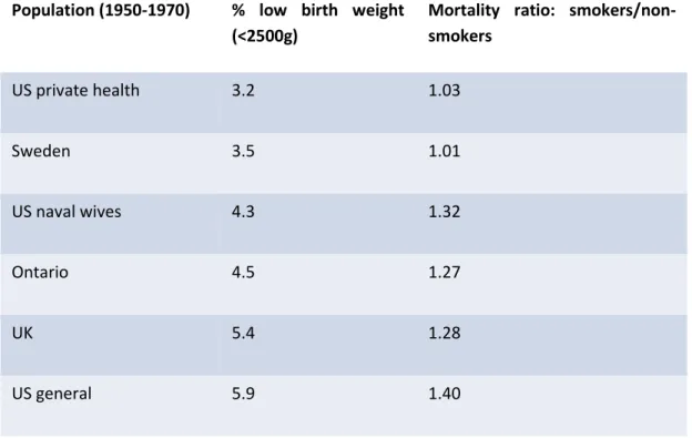
in a population with high average birth weight this relationship is known to be weak with a very large sample size needed to have reasonable power to detect it (see for example, Goldstein, 1977). Selecting a sample that does not represent a real population but has a high degree of heterogeneity in terms of birth weight, may provide much more power to investigate the hypotheses of interest. We can illustrate this particular point from an analysis of early studies that looked at the relationship between maternal smoking and neonatal or perinatal mortality. Goldstein (1977) showed that, for different studies representing different populations of pregnant women, the difference in (or ratio of) mortality rates between smokers and non-smokers increased steadily as the average birth weight in the population decreased. Table 1 shows this for six different studies. The simplest explanation for the relationship is that smoking acts on mortality through an average 160greduction in birth weight. The relationship between mortality and birth weight is nonlinear, with the relationship becoming steeper as birth weight decreases, and this implies that we will observe a greater difference for those populations with more low birth weight babies. In fact, for the two populations with the highest average birth weight, the difference is negligible.
Thus, if we had confined ourselves to the ‘marginal’ relationship between smoking and mortality, then our inferences would have differed according to the ‘real’ population studied. From a scientific perspective however, such inferences, especially in terms of a causal relationship, would be inadequate. It illustrates the point that, from a scientific perspective, the real population is of secondary importance: what we need is to understand those factors that could mediate the relationship of interest.
Table 1. Maternal smoking in pregnancy and neonatal/perinatal mortality
Population (1950-1970) % low birth weight (<2500g)
Mortality ratio: smokers/non-smokers
US private health 3.2 1.03
Sweden 3.5 1.01
US naval wives 4.3 1.32
Ontario 4.5 1.27
UK 5.4 1.28
US general 5.9 1.40
A case where both specific population estimates are required and there is sufficient power to explore scientifically interesting hypotheses, is the British birth cohort known as ‘Life Study’ (Dezateux et al., 2013). This has a design that studies all
451
together with a UK random sample over the same time period, of some 20,000 live births, treated as a random sample from the superpopulation defined over the whole country. Both components of the study are followed up during the first year of life (and potentially beyond) with considerable overlap in terms of the information collected. The pregnancy component aims to collect genetic and other biological data not collected in the birth component. The advantage of such a design is that for population estimates using variables collected in the birth component there is additional information available from the numerically larger pregnancy component to improve the accuracy of these, for example using suitable weights that can be computed from nationally available birth data. For many scientific hypotheses the data available from the pregnancy component alone will often suffice, but power can also be increased by using the data from the birth component, within a combined analysis. Furthermore, informative selection, notably as a result of non-response, can be addressed by the existence of comprehensive population birth registry data against which the characteristics of those responding can be checked. This is in effect a special case of purposive sampling. The ability to exploit such a design requires appropriate software tools that can ‘borrow strength’ across the two components. Providing such tools for routine data analysis is highly desirable, although it may be practicallychallenging. The point, however, is that it helps to understand the debate over whether a sample should be purposive or representative since in this case it can efficiently be both.
Conclusions
The idea that population studies, especially longitudinal ones, should strive to be representative of ‘real’ populations may not always be helpful. While, for certain purposes associated with enumeration and administrative policies, real population representativeness is required, from a scientific perspective this may well be unnecessary. Scientific inferences are concerned with uncovering relationships that can be tested across different contexts and that may eventually attain the status of causal explanations. To ensure validity researchers need to pay attention to selection factors that may lead to biased estimates, where ‘bias’ is defined in terms of a clearly defined
statistical (super)population, and much of applied
statistical methodology is devoted to this issue. To enhance the effectiveness of any analysis, heterogeneity is generally desirable, and this will often imply purposive sampling that is non-representative of any particular real population. In practice, as is the case with Life Study, an optimum design may well be one that combines such purposive sampling with population representativeness, so serving both enumeration and scientific aims.
Acknowledgements
My thanks for comments are extended to the following: Carol Dezateux, Francesco Sera and Rachel Knowles. The paper is based upon one delivered at the SLLS 2014 conference in Lausanne. This work was supported in part by the Economic and Social Research Council [Grant number ES/L002353/1]. Life Study is supported by the Economic and Social Research Council (ESRC), the Medical Research Council (MRC) and University College London (UCL) and is part of the Birth Cohort Facility Project, which receives funding from the UK Government's Large Facilities Capital Fund.
References
Dezateux, C., Brockelhurst, P., Burgess, S., Burton, P., Carey, A., Colson, D., Dibben, C., Elliot, P., Emond, A., Goldstein, H., Graham, H., Kelly, F., Knowles, R., Leon, D., Lyons, G., Reay, D., Vignoles, A., & Walton, S. (2013). Life Study: a UK-wide birth cohort study of environment, development, health, and wellbeing. The Lancet, 382, S31. http://dx.doi.org/10.1016/S0140-6736(13)62456-3
Ebrahim, S. & Davey-Smith, G. (2013). Commentary: should we always be deliberately non-representative?
International Journal of Epidemiology, 42, 1022-1026. http://dx.doi.org/10.1093/ije/dyt105
452
Goldstein H. (1977). Smoking in Pregnancy: some notes on the Statistical Controversy. British Journal of
Preventive & Social Medicine 31 13-17. http://dx.doi.org/10.1136/jech.31.1.13
Nohr, E.A., & Gleen, J. (2013). Commentary: Epidemiologists have debated representativeness for more than 40 years – has the time come to move on? International Journal of Epidemiology, 42, 1016-1017.
http://dx.doi.org/10.1093/ije/dyt102
Richiardi, L., Pizzi, C.F. & Pearce, N. (2013). Commentary: representativeness is usually not necessary and often should be avoided. International Journal of Epidemiology, 42, 1018-1022.
http://dx.doi.org/10.1093/ije/dyt103
Rothman, K.J., Gallacher, J.E.J., & Hatch, E.E. (2013a). Why representativeness should be avoided.
International Journal of Epidemiology, 42, 1012-1014. http://dx.doi.org/10.1093/ije/dys223
Rothman, K.J., Gallacher, J.E.J., & Hatch, E.E. (2013b). When it comes to scientific inference, sometimes a cigar is just a cigar. International Journal of Epidemiology, 42, 1026-1028.
453
Commentary by
Peter Lynn
University of EssexThe need for representative survey samples
Introduction
In any field of scientific endeavour it is healthy to challenge orthodoxy. Standard practice should not be assumed to be best practice without question. Representative sampling is the orthodoxy in many applied fields of survey research and it is pleasing that this special section
of Longitudinal and Life Course Studies is
questioning when and why this should be the case. Let us be clear what this debate is not about. It is not about how to select a representative sample. There is a long history of debate on that subject, going back at least as far as the foundation of modern survey sampling theory with Kiaer (1897) and Neyman (1934), given prominence following the 1948 United States Presidential Election polling disaster (Mosteller, Hyman, McCarthy, Marks & Truman, 1949), and periodically revisited in various forms ever since. My thoughts on the role of non-probability sampling are recorded in Lynn (2005). That debate is again topical currently, particularly due to the rise of relatively cheap and fast online access panels in the social and political sciences (Bosnjak, Das & Lynn, 2015). However, the topic here is not how to select a representative sample but rather when and why it should be our objective to do so.
What should a sample represent?
Survey samples are rarely if ever of inherent interest. Rather, a sample is used to make broader inferences. Therefore, survey samples should be representative of something broader. But what? Goldstein’s article touches upon this question by drawing distinctions between descriptive and analytical statistics and highlighting the role of confounding (or mediating) variables. I would suggest that if the analytical objective is to estimate the association between a particular set of variables, then the sample should be representative of that association. If the objective is to estimate a population distribution of some kind (be that
univariate or multivariate) then the sample should be representative of that distribution. And so on. If the sample is not representative of the set of parameters to be estimated, whether those are causal, associative or descriptive, then we risk biased estimation, in the statistical sense outlined by Goldstein. It could therefore be argued that the representativeness objectives for a survey sample should depend on the analytical objectives1.
454
ensure that the sample broadly covers the distribution of interest. However, this begs the question: which distribution? To be able to truly generalise our findings, we surely mean the distribution of values that could exist in any population to which we wish to claim that our results apply. Thus, we cannot completely get away from the notion of populations.These criteria for being able to rely on a non-representative sample are quite demanding. It is hard to envisage a realistic social science research example where we can be confident of knowing in advance all possible confounding variables (let alone being able to measure them all well). When the causal mechanism of interest is, say, biological or chemical, one may be able to get closer to meeting these criteria - and that is a possible reason for epidemiologists to have a different take on this debate to social scientists - but the fundamental issues are the same.
Most social surveys – even those tightly focused on a single topic – have multiple analysis objectives. Large numbers of estimates of different kinds are typically required, making it unlikely that all confounding mechanisms are known for all analyses. In this situation, as pointed out by Goldstein, a population representative sample will at least provide a means of identifying the form of unexplained variation, testing in an exploratory way the association of this variation with other variables, andthereby moving towards the advancement of knowledge about hitherto unidentified causal factors. The primary purpose of some surveys – and secondary purpose of many – is to provide a data resource for research by secondary analysts. It is impossible for such research to have been specified prior to the original design of the survey and therefore to have influenced the survey design. In this situation, having a population representative sample can be thought of as a safety mechanism that ensures that the population distribution of the phenomena of interest is covered and also permits estimation of the extent and nature of unexplained variation. Of course, it remains up to the researcher to decide whether the particular population covered is suitably similar to, or representative of, the kind of population to which inferences should be made. I return to this issue below.
Which Population?
The ultimate objective of most survey-based research is to inform policy or practice of some kind. With this in mind, my earlier statement about wanting a sample to be representative of the parameters of interest can be re-cast. The parameters of interest are those in the population(s) that will be affected by policy or practice. Let’s refer to this population as the
policy population2. So, broadly, we want our
survey sample to be representative of the policy population in terms of the parameters to be estimated. How can we be sure that this is the case? We can’t. Not least because the policy population is always, by definition, a future population and we can never perfectly predict the future. But there are two things we can do:
a) try to minimise the risk that our parameters of interest differ greatly between the study population and the policy population, by defining the study population appropriately;
b) try to predict or model relevant ways in which the policy population may differ from the study population and incorporate this into our estimation.
Step a) is typically achieved by studying the most recent available equivalent of the relevant future population. Thus, in 2015 we may be able to analyse data from a representative sample of the 2014 population of Great Britain, for example, in order to infer the likely effects of a policy that might be implemented in 2016. Our assumption is that the 2016 population will be broadly similar to the 2014 one in terms of the relevant (causal) parameters. However, we do not expect the population structure to be identical: based on recent trends, we may expect some net ageing and some net immigration, for example, in which case we can implement step b) by projecting our estimated parameters onto the predicted 2016 population structure.
455
impacts, so the true policy population perhaps consists of people resident in Britain at any time over the subsequent several years or decades. And often study and policy populations are even further disconnected. For example, if a good survey-based study has been carried out in one country, should researchers and policy-makers in another country assume that the findings will apply to their situation too? This is a common dilemma.Funders must decide whether it is worth investing considerable resources to replicate a study carried out in a different context. They should be guided by the principles set out above. It is only worth funding the replication study if there is a sufficiently strong probability that the key parameters of interest are substantially different. Interpreting concepts such as “sufficiently strong probability” and “substantially different” will of course be subjective, but can be guided by knowledge of pertinent differences between the two populations and, particularly, by study findings regarding important confounders and unexplained variance.
Relevant policy populations can be very different for different types of research. Medical researchers may often hope that their findings could be generalisable to almost all current and future human populations (barring changes in the underlying etiology), whereas public bodies concerned with administering healthcare, education, housing, social support and so on are generally responsible for populations that are clearly defined by geography, usually at a national, regional, or local level. In the latter case, researchers may use survey samples that are representative of a recent equivalent of the same geographically-defined population or may resort to similarity-of-parameters arguments in using data from a different population (for example, arguing that national findings should apply in each region of the country).
Longitudinal Surveys
The arguments that I have presented so far are rather general and should apply to any sample-based scientific endeavour. However, longitudinal studies in the social sciences have at least three additional distinct characteristics that should influence the answer to the question posed in the title of Goldstein’s paper:
a) Longitudinal estimates by definition refer to longitudinal populations;
b) The time interval between data collection and policy impact can be particularly great;
c) During the course of the study, new research agendas can emerge that were not envisaged when the study was initially designed.
I discuss here each of these three points in turn. Any human population (‘real’ population, in Goldstein’s terms) is dynamic; people will join or leave the population over time. Analysts of cross-sectional surveys tend to ignore this
456
not by just a couple of years, as in the example of the previous section, but by four decades or more. This makes it harder for the researcher to be confident that key population parameters will remain unchanged: in a rapidly-changing world, not only may feeding practices themselves have changed, but so might the many mediators of their impacts on early-adulthood outcomes. Research agendas certainly evolve over time, due to new knowledge, new technology, new social problems, and so on. When the sample design for the National Child Development Study (NCDS) was established, in the 1950s, it would have been impossible to envisage the myriad purposes for which researchers would be using the data half a century later. For this reason, the role of population representative sampling in ensuring the sample will contain as much heterogeneity as exists in the population is particularly important. The heterogeneity will be present for any research objective, not just those that were identified when the study was conceptualised.Conclusion
The omission of the word ‘population’ from the title of this piece is deliberate: survey samples certainly need to be representative, but not necessarily of a conventionally-defined population. To meet scientific objectives, samples
should represent the estimation parameters of interest. How this is best achieved will depend largely on how much is known about these parameters prior to the study. When little is known, and particularly when some research objectives cannot be well specified in advance, population representative sampling provides a mechanism for ensuring representation of extant variance. For multi-purpose surveys, population representative sampling is likely to represent an efficientcompromise between the diverse optimal sample distributions for different analytical purposes. The sample should represent a population that is as similar as possible to the future policy population(s) that may be affected by study findings. A good choice may be a recent equivalently-defined population, especially when this maximises overlap between the study population and the policy population.
Longitudinal studies are typically characterised by the features that point towards population representative sampling as an appropriate strategy (limited advance knowledge about estimation parameters, inability to specify all estimation requirements in advance, large time interval between data collection and policy implementation).
References
Bosnjak, M., Das, M. & Lynn, P. (2015). Methods for probability-based online and mixed-mode panels:
Selected recent trends and future perspectives. Social Science Computer Review. Published online 7 April 2015. http://dx.doi.org/10.1177/0894439315579246
Kiaer, A.N (1897). The Representative Method of Statistical Surveys. Translation 1976, Norwegian Central Bureau of Statistics, Oslo.
Kruskal, W. & Mosteller, F. (1979). Representative sampling III: the current statistical literature.
International Statistical Review 47(3), 245-265. http://dx.doi.org/10.2307/1402647
Lynn, P. (2005). Inferential potential of non-probability samples: discussion. Bulletin of the International
Statistical Institute, Proceedings of the 55th Session. Sydney: International Statistical Institute.
Lynn, P. (2011). Maintaining cross-sectional representativeness in a longitudinal general population survey. Understanding Society Working Paper 2011-04, Colchester: University of Essex. https://www.iser.essex.ac.uk/research/publications/working-papers/understanding- society/2011-04
Mosteller, F., Hyman, H., McCarthy, P.J., Marks, E.S. and Truman, D.B. (1949). The Pre-election Polls of 1948. New York: Social Science Research Council.
Neyman, J. (1934). On the two different aspects of the representative method: the method of stratified sampling and the method of purposive selection (with discussion). Journal of the Royal Statistical
457
Smith, P., Lynn, P. & Elliot, D. (2009). Sample design for longitudinal surveys. In Lynn, P. (Ed.),
Methodology of Longitudinal Surveys, 21-33. Chichester: Wiley.
http://dx.doi.org/10.1002/9780470743874.ch2
Endnotes
1
Kruskal and Mosteller (1979) distinguish estimation bias from selection bias. Goldstein notes that unbiased estimators can be constructed from biased samples, provided the biasing selection mechanism is known, as with the case of disproportionate stratified probability sampling. In this brief note I shall fudge this issue: my use of the term population representative sample includes – but is not necessarily limited to – any probability-based sample that covers the whole population.
2
458
Commentary by
Graciela Muniz-Terrera
University of Edinburgh, UKRebecca Hardy
University College London, UKSome thoughts about representativeness
The paper by Goldstein makes an important additional contribution to the ongoing debate about whether and when analytic samples need to be population representative in studies in epidemiology and social and medical research. The paper outlines the arguments presented by Rothman, Gallacher and Hatch (2013) and the stimulating accompanying commentaries that initiated the recent discussion on the topic. The need to distinguish between a “real” population and a population defined as a statistical concept that refers to any well-defined collection of units, but that may not reflect any actual population is also discussed. Additionally, Goldstein recalls the definition of bias as the difference between estimates obtained from any particular sample and the unknown true parameter of the population under study, emphasising that this population only has to be a statistically defined population and not a “real” population. In this paper, we comment on a number of points which have particular relevance for birth cohort and longitudinal studies.
The discussion of the temporal aspect of the concept of representativeness is, of course, important. Goldstein points out that representativeness is not a static concept that is preserved indefinitely over time, but rather, is a concept affected by the passing of time. Even when all efforts are made to select a representative sample of a given population at the outset of a study, the representativeness of this initial sample is unlikely to be preserved over time as the sample is followed up longitudinally. The real population of which the sample was initially representative will inevitably evolve, while at the same time loss to follow up will alter the characteristics of the study sample. Goldstein cites the example of the ‘Life Study’, the newest of the British birth cohort studies, where a complex sampling strategy and the use of weighting allows both the estimation of population parameters with adequate accuracy and the investigation of scientific hypotheses in a group
with more extensive biological data. Let us now consider the oldest of the British birth cohort studies, the MRC National Survey of Health and Development (NSHD) (Wadsworth, Kuh, Richards & Hardy, 2006). The NSHD followed up a sample of all single births to married women in England, Scotland and Wales which took place in one week in March 1946. This initial sample included all babies born to women with husbands in non-manual and agricultural employment and one in four births to women with husbands in manual employment. This sampling scheme was chosen to keep the national distribution and to achieve a similar proportion of children in each social group (Wadsworth, 1991). Weights have thus been used when calculating prevalence estimates in order to allow for this original sampling. In 2015, the cohort is now aged 69 and the 24th data collection on the whole sample is taking place. Of course, the NSHD sample are no longer representative of the population of individuals aged 69 years old now living in England, Scotland and Wales. Demographic changes have occurred, with both immigration and emigration taking place over the lifetime of the cohort. Hence, any prevalence estimates can only ever be representative of the British-born population of 69 year olds. Furthermore, the diverse origins of immigrants joining the British population will mean that they have been exposed to different early life conditions compared with the British born population. Such differences in early life experience are likely to impact on adult health and mortality patterns and could thus affect estimates of association between early life risk and adult outcomes.
459
Cohort, during childhood, as cohort members could be traced through schools, immigrants born in the reference week were added to the samples. This was no longer possible once cohort members became adults (Power & Elliott, 2006, Elliott & Shepherd, 2006). We appreciate the value of such attempts to retain representativeness, but also see challenges in this practice if the distribution of the subgroups that comprise the original population is also dynamic and vary significantly over time. The innovative design of the ‘Life study’ (Dezateux et al., 2013) means that the initial sample is both “purposive and representative” and it will be informative to see how appropriate software tools for routine and complex data analysis can be provided. It will also be interesting to see whether representativeness can be maintained as the sample is followed up longitudinally, as loss to follow up and continuous demographic changes to the population occur. Given the richness of the data available in cohort studies and their ability to address unique scientific hypotheses about long term associations, we need to consider whether attempting to retain representatives by sample supplementation or by statistical weighting for investigations of prevalence is the best use of such studies.In the original exchange between Rothman and others, Elwood (2013) elaborated the concept that any real population is a historical entity and that by the time inferences about the population are available, the initial population may have changed in important ways. We now reflect on how period effects can affect inferences made using historical data. As an example, let us consider the association of smoking and cognitive function in school pupils aged 15. Assume we have data for two samples of children that were representative of the school population aged 15 at the time of data collection, such that one sample comprised of students aged 15 years old in 1982 and the other of students aged 15 in 2013. Smoking prevalence in these two samples born 30 years apart will vary greatly. In 1982, 24 % of pupils aged 15 smoked, a percentage that has been decreasing steadily over time so that by 2013 only 8 % of pupils smoked (www.ash.org.uk) as a consequence of heightened awareness of its negative effects on health and various changes in laws, public health and commercial policies. A lack of power to detect an effect of smoking on cognitive function could
therefore result as the prevalence of the risk factor declines. So, even when both samples were chosen to be representative of the population of pupils aged 15, because of a period effect, different conclusions about the association of interest could be drawn. If the researcher is interested in the potential causal association between smoking and cognition, then selecting a population with a higher prevalence of smoking is more important than picking one which is representative. On the other hand a risk factor might become more prevalent over time and thus associations may not be picked up in historical cohorts. For example, the prevalence of childhood obesity was considerably lower in the NSHD compared with cohorts born in the 1990s and later (Johnson, Li, Kuh & Hardy, 2015). It is therefore unclear whether the generally null associations between body mass index (BMI) in early childhood and coronary heart disease (CHD) observed in historical cohorts (Owen et al., 2009) are due to a lack of power. Such historical differences need to be considered and discussed when, for example, synthesizing results in systematic reviews and when implementing evidence based public health policies.
460
reproducible research has, historically, been at the core of scientific discovery.From that perspective, the need to generate strong evidence about patterns of associations is at the core of the multi-study work fostered by the Integrative Analysis of longitudinal Studies of Ageing network, a network of longitudinal studies of ageing (www.ialsa.org). Researchers affiliated to the IALSA network independently analyse data from multiple studies employing a coordinated approach that involves the consistent use of the same analytical method (identical analytical model where possible and consistent coding of harmonized variables where possible). This coordinated analytical approach maximises the ability to fairly compare results and enables the examination of consistency of patterns and of associations across samples that may differ in a variety of ways, including differences by geographical location, sample composition and representativeness (Piccinin). The use of the same analytical approach reduces the potential sources of heterogeneity across studies that may emerge from the use of different statistical methodologies to answer similar questions. Consistent results generated from diverse samples are reassuring and provide stronger evidence in support of the hypothesis tested. On the other hand, inconsistent results require a thoughtful evaluation of potential reasons that may explain the divergence of results, including differences that may emerge from features of the data (including representativeness), and sample composition and sampling procedures. For example, in an investigation of the association of
the effect of education, age and sex on global cognitive function measured using the Mini Mental State Exam in six international longitudinal studies of ageing, Piccinin and colleagues (2012) found that education was positively associated with performance across all six studies, but was only associated with rate of decline in the cohort containing the oldest participants. In five of the six studies, estimates of rate of decline were also found to be similar, but in the cohort of oldest individuals, individuals were found to decline at a much faster rate than in the other samples. The authors report that an investigation of the sample composition and a better examination of the sampling procedure followed in this outlying study helped them understand that dementia cases had been handled differently in the study compared to the other studies. Indeed, in this study efforts had been made to keep individuals who developed dementia in the study, whereas in all the other studies individuals with dementia were not included in the follow up samples. When individuals with dementia were removed from the sample, the estimated rate of decline aligned to the rate of decline estimated in the other five studies.
The general discussion about representativeness and Goldstein’s contribution with particular
relevance to longitudinal studies and their historical context is very valuable. This discussion is helpful in raising awareness among researchers to think more about when representativeness is a problem, but also to appreciate when to value a lack of
representativeness.
References
Dezateux, C., Brockelhurst, P., Burgess, S., Burton, P., Carey, A., Colson, D., Dibben, C., Elliot, P., Emond, A., Goldstein, H., Graham, H., Kelly, F., Knowles, R., Leon, D., Lyons, G., Reay, D., Vignoles, A., & Walton, S. (2013). Life Study: a UK-wide birth cohort study of environment, development, health, and wellbeing. The Lancet, 382, S31. http://dx.doi.org/10.1016/S0140-6736(13)62456-3
Drummond, C. (2009). Replicability is not Reproducibility : Nor is it Good Science. Retrieved from: www.site.uottawa.ca/ICML09WS/papers/w2.pdf
Elliott, J. & Shepherd, P. (2006) Cohort profile: 1970 British Birth Cohort (BCS70). International Journal of
Epidemiology, 35(4), 836–843. http://dx.doi.org/10.1093/ije/dyl174
Elwood, J.M. (2013). Commentary: On representativeness. International Journal of Epidemiology, 42(4), 1014–1015. http://dx.doi.org/10.1093/ije/dyt101
Francis, G. (2012) Publication bias and the failure of replication in experimental psychology. Psychonomic
Bulletin and Review 19(6), 975-991. http://dx.doi.org/10.3758/s13423-012-0322-y
Ioannidis, J.P.A., Nosek, B. & Iorns, E. (2012). Reproducibility concerns. Nature Medicine18(12),1736–7.
461
Johnson, W., Li, L., Kuh, D. & Hardy, R. (2015). How Has the Age-Related Process of Overweight or Obesity Development Changed over Time? Co-ordinated Analyses of Individual Participant Data from Five United Kingdom Birth Cohorts. PLOS Medicine, 12(5), e1001828.
http://dx.doi.org/10.1371/journal.pmed.1001828
McNutt M. (2014). Reproducibility. Science. 343(6168),229. http://dx.doi.org/10.1126/science.1250475
Mulkay, M.& Gilbert, G.N. (1986) Replication and Mere Replication. Philosophy of the Social Sciences16(1), 21–37. http://dx.doi.org/10.1177/004839318601600102
Owen, C.G., Whincup, P.H., Orfei, L., Chou, Q.A., Rudnicka, A.R., Walthern, A.K. … Cook, D.G. (2009). Is body mass index before middle age related to coronary heart disease risk in later life? Evidence from observational studies. International Journal of Obesity, 33(8), 866–877.
http://dx.doi.org/10.1038/ijo.2009.102
Piccinin, A.M., Muniz-Terrera, G., Clouston, S., Reynolds, C.A., Thorvaldsson, V. Deary, I.J. …Hofer, S.M. (2012).Coordinated Analysis of Age, Sex, and Education Effects on Change in MMSE Scores. The
Journal of Gerontologly Series B: Psychological Sciences and Social Sciences, 68(3), 374-390.
http://dx.doi.org/10.1093/geronb/gbs077
Power, C. & Elliott, J. (2006). Cohort profile: 1958 British birth cohort (National Child Development Study).
International Journal of Epidemiology, 35, 34–41. http://dx.doi.org/10.1093/ije/dyi183
Rothman K.J., Gallacher, J.E.J. & Hatch, E.E. (2013). Why representativeness should be avoided. International
Journal of Epidemiology 42(4), 1012-1014. http://dx.doi.org/10.1093/ije/dys223
Wadsworth, M. Kuh, D., Richards, M. & Hardy, R. (2006). Cohort profile: The 1946 National Birth Cohort (MRC National Survey of Health and Development). International Journal of Epidemiology 35(1), 49-54. http://dx.doi.org/10.1093/ije/dyi201
462
Commentary by
Colm O’Muircheartaigh
University of Chicago, USWhy we need population representative samples
Goldstein questions the need for observational studies to achieve representativeness for well-defined populations, in particular for longitudinal studies. While he recognises the distinction between the notions of representativeness and proportionality, he fails to acknowledge the importance of distinguishing between samples of convenience and targeted samples from special subpopulations. In this note I emphasise the critical significance of probability sampling, in contrast to purposive sampling, and draw special attention to the artificial distinction between descriptive and analytical statistics. Goldstein (correctly) draws attention to the confusion between disproportional sampling and non-representative sampling but fails to recognise the inferential implications of choosing between probability samples and nonprobability samples. A probability sample is in essence a sample in which every element of the population has a (known) non-zero probability of selection; the definition of the population may be such that it does not correspond to a real population. The structure of a probability sample from a (general) population may exclude some domains from the target population and may be modified by design in order to produce appropriate numbers of cases for particular comparisons of subsamples of that target population. Probability samples have particular strength in making inferences, whether for scientific or for policy purposes.
Defining populations
All inference is, by definition, to a population beyond the sample on which the inference is based. Much of the argument in Goldstein, and in the papers he references, has to do with the definition of this inferential population. I concur that the population must be clearly defined; I accept also that it may not correspond to a “real” population at a point in time. However, unless it can be defined in such a way that a sample may be selected from it, there will be no scientific foundation for inferences to it without untestable assumptions about freedom from bias.
Consider first the case where the purpose is to represent a national population; as an example, consider the selection of a sample for the United States (US) National Children’s Study (NCS)(Michael & O’Muircheartaigh, 2008). In designing a nationally representative sample for this study, the purpose is not to address every subpopulation of interest in the US. The purpose is to insure that every element in the population has a non-zero probability of being selected into the sample. This is achieved by identifying a survey population that is defined to be as close to the target population as feasible, such that it reflects both measurable and unmeasurable characteristics of that population
Suppose that we are interested in the relationship between an environmental exposure X and a health outcome Y, which can be modeled (for simplicity) as the linear function Y=a+bX+e. If all people in the population have the same b, then the nature of the sample does not matter because as long as X is accurately measured we will have only random measurement error in Y. However, if there are confounding factors Z, which affect Y and are related to X, then our estimate of b may be biased unless the elements of Z are controlled. If Z is known, then model-based estimates of the relationship between X and Y can be obtained that control for Z and yield an unbiased estimate of b, again regardless of the sampling design. However, there may also be moderator variables W, which interact with X in influencing Y. Here, different individuals will have different values of b depending on the elements in W. If W is known, then we can include interactions in the model and the separate estimates of b will also be unbiased.
463
fully reflects the population of interest, a probability sample drawn from the population so that our estimate of b is an unbiased estimate of the average effect in the population or in a defined subgroup. The probability sample guarantees that we will (in expectation) cover the range of confounding variables proportionately.It is also possible that the interest is not in the average effect but in the effect on specific subgroups of this general population (as in the birth weight example below). Thus, in the NCS we might wish to focus on particular ethnic groups or on the comparison of these groups. In this case to maximize power for the comparison we would take equal numbers of cases from the groups of interest, rather than numbers proportional to their distribution in the general population. These subsamples would however be chosen to be representative of the groups of interest; their representativeness would be warranted by the fact that they were probability samples from their respective groups. Only the relative sizes of the subsamples would deviate from the parent population, not the intrinsic nature of the sampling process.
Goldstein’s example of the relationship between pregnancy smoking and neonatal mortality provides a further illustration of this principle. The six studies he cites (from an analysis by Goldstein (1977)) demonstrate a non-linear relationship between mortality and birth weight, with a negligible effect for the two populations with the highest average birth weight, and an increasingly steep relationship as the population average birth weight decreases. Goldstein argues that this example demonstrates the secondary importance of the population. To the contrary, the data demonstrate the opposite. Had the range of birth weights across the US been included in a single US study, the analysts might have been more likely to observe the non-linearity in the relationship; this indicates the importance of covering the full range of variation of X, W, and Z in a population rather than accepting the subpopulation that is most convenient. One might indeed argue that there was a failure of both the theoretical basis and the analysis of the studies in not examining the data for possible interactions with birth weig
ht in the model,
At no point in his disquisition does Goldstein suggest that the samples in any of the studies he
cites should be “non-representative”. The implicit understanding is that the sample in each is in fact representative of the population from which it is drawn. Were it not, neither the partial generalisation within the study would be justified, nor would its incorporation into Goldstein’s 1977 meta-analysis.
Two-phase sampling
The case of the British birth cohort known as the ‘Life Study’ is also subject to an alternative interpretation from that offered in Goldstein. A geographically clustered sample of 60,000 mothers is selected from a set of relatively small but geographically heterogeneous clusters; the 60,000 mothers are assumed to constitute a random sample from a set of geographic strata; there is a parallel (random) UK sample of 20,000 live births. The two samples can be used together to “borrow strength” from each other for different analyses. Comprehensive national (population) data from birth registries can be used to correct for differential nonresponse.
This combining of samples with different characteristics and different intensity of measurement is well recognised as a powerful design. The classic two-phase sampling design (Neyman, 1938) proposes just this combination of general representation and subsample focus; Neyman visualizes both samples as probability samples. Goldstein proposes this as a special case of purposive sampling, though it is not clear what his argument is. Presumably he does not argue that selecting the geographical areas purposively is superior to a design in which the areas were selected on a probability basis from a properly constructed frame of geographical areas. If indeed the selected areas were for some reason the only areas available, then suspicion must attach to them as being unrepresentative even of areas with ostensibly equivalent characteristics.
The extent to which the combined sample can be justifiably used to make inferences to the whole population depends critically on either (i) both samples being probability samples, or (ii) model-based assumptions that allow generalisation from the purposive component to the whole.
Additional benefits of representation
through probability sampling
464
Hypotheses about new exposures and gene-by-environment moderation will arise over the next 20 years, and a probability sample provides the best insurance that the study will provide useful numbers of children with variation in those environments and exposures of interest. The probability design also increases the prospects for serendipity by maximizing the spread of W and Z in the sample.Maximization of scientific acceptability of data
and of discoveries across disciplines
While many disciplines do not require probability samples for their inferences, no discipline considers a probability sample to be inferior to an alternative. Thus data based on a probability sample maximize the potential for cross-disciplinary collaboration and publication.
Public and political/policy acceptance
Resource allocation and acceptability of discoveries will be greater if the data are based on a
scientifically warranted representative sample of the population.
Full variation in risks and exposures
A probability sample will produce generalisable risk estimates and the capability to estimate policy/intervention benefits from associations discovered and reported from the study.
Conclusion
Investigations of all kinds can make a contribution to science, and samples that are not representative have a place in scientific research, especially at early stages of exploration. I contend however that the superficial message of Goldstein’s excellent article is wrong. Ceteris paribus, for both science and policy a probability sample is superior to a non-probability sample, representation trumps convenience, and the best way to obtain representation of the population of interest is through probability methods.
References
Michael, R. & O’Muircheartaigh C. (2008). Design Strategies and Disciplinary Perspectives: the Case of the US National Children’s Study. Journal of the Royal Statistical Society, Series A, 171(2) 465-480.
http://dx.doi.org/10.1111/j.1467-985X.2007.00526.x
Neyman, J. (1938). Contributions to the theory of sampling human populations, Journal of the American
465
Commentary by
Chris Skinner
London School of Economics, UKDiscussion of ‘When and why do we need population representative samples?’
There is much wisdom in this paper by Harvey Goldstein which builds on discussion in a set of papers in the International Journal of Epidemiology (IJE), and applies the ideas developed to a new British birth cohort study, the Life Study. I shall focus on his main theme, which rejects the need for representative samples, and on his concluding remarks relating to the Life Study. My comments come particularly from a survey statistics perspective.
I was reminded in looking at the papers in IJE of the observation by Kruskal and Mosteller (1979) (and in their three related articles) that the term ‘representative sample’ has multiple uses and “because of its ambiguities and imprecision”, they “recommend great caution” in the use of this term and “usually a more specific expression will add clarity” (p.13). I shall seek to make greater use of the expressions ‘population’, ‘sample’ and ‘bias’ in my discussion.
As I understand Goldstein’s main concern about representative sampling, it is that, for scientific purposes, making inference about ‘real’ populations is of secondary importance. This is a position which I should like to question. The survey statistics literature does make a distinction between descriptive/enumerative and analytic/scientific uses of surveys/studies. Estimation for a single study population is a common primary objective for the former. For the latter, the focus of Goldstein’s paper, I think the notion of population will invariably need further refinement, but I think it can still serve a useful purpose to specify collections of units underlying targets for inference. I do not feel the need to downplay the notion of ‘real’ population.
Perhaps the simplest definition of populations of interest for scientific purposes is where there are two subpopulations to compare. I conceive of these subpopulations as ‘real populations’ in Goldstein’s terminology. Suppose, for example, we wish to undertake a comparison of an outcome Y, according to values of X, given confounding factors Z (say infant mortality by maternal smoking given birth
weight in Goldstein’s example). For such conditional analysis, it would be natural to define specific subpopulations by X and Z, between which comparisons are to be made. Thus, in the example, one might choose to compare a low birth weight subpopulation and a normal birth weight subpopulation. Such comparisons have many vital roles in scientific research, as Goldstein notes. They may help to elicit and test causal hypotheses, perhaps through control of confounding factors. They may be valuable in assessing the replicability of findings across populations or to learn about interactions.
Given the specification of such subpopulations, it will often make sense to sample these subpopulations with different sampling fractions. For example, as discussed by Goldstein, the power to investigate the analytic objectives may be improved by sampling the low birth weight subpopulation with a higher relative sampling fraction. But I do not see this observation as any reason why the subpopulations (as real populations) are of ‘secondary importance’. Their definition seems fundamental. I also do not see any reason why an analysis embracing a comparison of such subpopulations need be weighted to the population of all births (Skinner, 2005, p.84), let alone any need for the analysis to be confined to the ‘marginal’ relationship between smoking and mortality.
466
arises with, for example, households with the structure of the unit changing over time. In such cases, the term ‘population’ may seem stretched, but I think it is still reasonable to think in terms of what Goldstein calls a ‘well-defined collection of units’. Causal questions cannot be assessed from data on a single case but rather require reference to a set of units. As Holland (1986, p. 947) writes, “the important point is that the statistical solution [to the fundamental problem of causal inference] replaces the impossible-to-observe causal effect of t on a specific unit with the possible-to-estimate average causal effect of t over a population of units”. In my view the relevant populations do define ‘real’ notions of primary not secondary importance, given the need to report scientific findings transparently in terms of the kinds of people or other units to which they apply.I now turn to the role of sample selection. I have already noted, in agreement with Goldstein’s discussion, that it may often be sensible to allocate the sample differentially according to variables of scientific interest (X and Z above) with a view to improving sampling efficiency (i.e. reducing variance). Consider next the question of bias, as arising from differences between the characteristics of sample units and those in the population (as conceived of in the previous three paragraphs). I have in mind bias arising from purposive and other forms of non-probability sampling, for example the volunteer effects described by Ebrahim and Davey-Smith (2013). Such bias is of major concern to survey methodologists today, with the relentless push to adopt non-probability samples, such as in internet panels, for cost and other non-scientific reasons.
In summary, I do think that in the analysis of longitudinal studies it is desirable to specify collections of units as populations, with a clear scientific rationale, and that the potential biasing effects of sample selection are of primary concern. My final comments will elaborate on these points in the context of the Life Study. Here the basic study populations from which samples are drawn (leaving aside timing aspects) are (a) k populations of pregnant mothers (and partners) associated with k maternity units and (b) the population of all live births in the UK. I am unclear about the value of k (perhaps it remains to be determined) but suppose that it is small (under 10?). Sampling in (a) is by census and in (b) by a standard probability scheme
and so, for the purpose of current discussion and leaving aside non-response considerations, I think we can disregard issues of representative sampling within these populations.
In the context of the earlier discussion, the key issue relates to the purposive selection of the maternity units. Following Goldstein’s discussion, it seems natural to ask what is the scientific rationale for the choice of maternity units? From Goldstein’s paper, the rationale seems to be geographic heterogeneity, perhaps associated with differences in distributions of what I have called X and Z variables relevant to the study. This raises the question of how differences in findings between different maternity units are to be interpreted? If, for example mortality ratios vary between units as in table 1 and there is also significant variation between units in a large number of other maternal health and socioeconomic factors, how will the finding be scientifically informative if k is small? Moreover, for some kinds of analyses, interpretation may even be complicated by confounding between the effect of the maternity unit and the nature of the maternal population. In any case, if the results of analyses of data from a given maternity unit are only to be reported as relating to that population then issues of external generalisability are avoided and I have no concerns about sample selection bias. There do not then seem to be any differences in questions of representativity/generalisability compared to other geographically specific studies, such as the Southampton Women’s Survey (Inskip et al., 2006). The fact that scientific studies have some spatial and temporal specificity seems inevitable.
The more difficult questions relate to how the data will be combined across populations. The statistical methodology for standard comparisons would seem straightforward. Thus, in a regression setting, one may construct a categorical covariate representing both the k maternity populations and the general ‘birth population’, the latter possibly broken down by region or in some other geographical way. I am still unclear how to interpret the coefficients of this covariate and associated interaction terms, but this is just the comparative question I have already asked above.