THE PROCYCLICAL EFFECTS OF BASEL II
Rafael Repullo and Javier Suarez
CEMFI Working Paper No. 0809
June 2008
CEMFI
Casado del Alisal 5; 28014 Madrid Tel. (34) 914 290 551 Fax (34) 914 291 056
Internet: www.cemfi.es
We would like to thank Sebastián Rondeau for his excellent research assistance and Matthias Bank, Jos van Bommel, Thomas Gehrig, Claudio Michelacci, Oren Sussman, Dimitri Tsmocos, Lucy White, Andrew Winton, and seminar audiences at the 2008 AFA Meetings, 2007 EFA Meetings, 2007 European, Far Eastern, and Latin American Meetings of the Econometric Society, Bank of Portugal Conference on “Bank competition”, ECB Conference on “The implications of changes in banking and financing on the monetary policy transmission mechanism”, ETH Zurich Conference on “Banking and the macroeconomy”, CEMFI, the Federal Reserve Board, the New York Fed, the Richmond Fed, the European University Institute, and the Universities of Berlin (Humboldt), Oxford, Tilburg, and Zurich for their comments. Financial
CEMFI Working Paper 0809 June 2008
THE PROCYCLICAL EFFECTS OF BASEL II
Abstract
We analyze the cyclical effects of moving from risk-insensitive (Basel I) to risk-sensitive (Basel II) capital requirements in the context of a dynamic equilibrium model of relationship lending in which banks are unable to access the equity markets every period. Banks anticipate that shocks to their earnings as well as the cyclical position of the economy can impair their capacity to lend in the future and, as a precaution, hold capital buffers. We find that the new regulation changes the behavior of these buffers from countercyclical to procyclical. Yet, the higher buffers maintained in expansions are insufficient to prevent a significant contraction in the supply of credit at the arrival of a recession. We show that cyclical adjustments in the confidence level behind Basel II can reduce its procyclical effects without compromising banks’ long-run solvency.
JEL Codes: G21, G28, E43.
Keywords: Banking regulation, Basel II, Business cycles, Capital requirements, Credit crunch, Loan defaults, Relationship banking.
Rafael Repullo CEMFI and CEPR [email protected]
Javier Suarez CEMFI and CEPR [email protected]
1
Introduction
A widespread concern about the new risk-sensitive bank capital regulation, known as Basel II, is that it might amplify business cyclefluctuations, forcing banks to restrict their lending when the economy goes into recession. Even in the old regime of essentially flat capital requirements of the 1988 Basel Accord (Basel I), bank capital regulation has the potential to be procyclical because bank profits may turn negative during recessions, impairing banks’ lending capacity. Additionally, the capital requirements prescribed by the Internal Ratings Based (IRB) approach of Basel II are an increasing function of banks’ estimates of the probability of default (PD) and loss given default (LGD) of each loan, and these inputs are likely to rise in downturns. So the concern about Basel II is that the increase in capital requirements during downturns might lead to a severe contraction in the supply of credit.
Two key conditions are necessary for these contractionary effects to occur. First, some banks must find it difficult to respond to the higher capital requirements by issuing new equity. Second, some of their borrowers must be unable to switch to other sources offinance.1
However, these conditions are not sufficient for the existence of significant procyclical effects, since banks anticipate that shocks to their earnings as well as the cyclical position of the economy can impair their capacity to lend in the future and, as a precaution, may hold capital in excess of the regulatory requirements. The critical question is whether capital buffers (that will endogenously respond to regulatory changes) will be sufficient to neutralize the procyclicality added by the new requirements.
This paper analyzes the cyclical effects of Basel II in the context of a tractable dynamic equilibrium model of relationship banking in which the business cycle is modeled as a two-state Markov switching process. At every date a continuum of entrepreneurs enters the market. They demand funds for two consecutive periods, giving rise to an overlapping generations structure. Consistent with the view that relationship banking makes banks privately informed about their borrowers, we assume that (i) borrowers become dependent
1These conditions have been noted by Blum and Hellwig (1995) and parallel the conditions in Kashyap, Stein, and Wilcox (1993) for the existence of a bank lending channel in the transmission of monetary policy.
on the banks with which theyfirst start a lending relationship, and (ii) banks with ongoing relationships have no access to the equity market. Thefirst assumption captures the lock-in effects caused by switching costs and the potential lemons problem faced by banks when a borrower is switching from another bank.2 The second assumption captures the implications of these informational asymmetries for the market for seasoned equity offerings, which can create prohibitive transaction and dilution costs for urgent recapitalizations. It is consistent with the view of the Basel Committee on Banking Supervision (2004, paragraph 757): “It may be costly for banks to raise additional capital, especially if this needs to be done quickly or at a time when market conditions are unfavorable.” It can also be seen as a convenient reduced-form for the observed delays in banks’ recapitalizations.3
The combination of relationship lending and the inability of banks with ongoing rela-tionships to access the equity market establishes a natural connection between the capital shortages of some banks at a given date and the credit rationing of some borrowers at that date. Yet, each cohort of new borrowers is assumed to be funded by banks that renew their lending relationships, have access to the equity market, and hence face no binding limits to their lending capacity.
In order to isolate the potential cyclicality coming from the supply side of the loan market, we abstract from demand-side cyclicality and aggregate feedback effects that might mitigate and exacerbate, respectively, the aggregate implications of the cyclicality in banks’ lending capacity. The model, however, could serve as a building block of a more comprehensive dynamic stochastic general equilibrium model in which, say, part of the production comes from entrepreneurial firms that require relationship bank finance.
We define equilibrium under the assumption of free entry into the banking sector, which implies that the banks’ net present value at the dates in which they can issue equity must be zero. We characterize the equilibrium loan rates and banks’ capital decisions in each
2See Boot (2000) for a survey of the relationship banking literature. Several papers explicitly analyze the costs of switching lenders under asymmetric information (e.g., Sharpe, 1990) as well as the trade-offs behind the possible use of multiple lenders as a remedy to the resulting lock-in effects (e.g., Detragiache et al., 2000). We are implicitly assuming that these alternative arrangements are prohibitively costly.
3Barakova and Carey (2001) study the time to recovery of US banks that became undercapitalized in the 1984-1999 period, showing that they needed an average of 1.6 years to restore their capital positions.
state of the economy, and derive a number of comparative statics results. Assuming that equity financing is more costly than deposit financing, we show that capital requirements increase equilibrium loan rates, but have an ambiguous effect on capital holdings. On the one hand, the higher prospects of ending up with insufficient capital call for the holding of larger buffers; on the other hand, higher capital requirements reduce the profitability of future lending, and thus the bank’s interest in preserving its future lending capacity. Our analytical expressions suggest that the shape of the distributions of loan losses in different states of the economy matter for determining which effect dominates. Since the impact of capital requirements on the supply of second period loans is, therefore, analytically ambiguous, we assess it numerically.
For the numerical analysis, we describe the distributions of loan losses according to the single risk factor model of Vasicek (2002), which provides the foundation for the IRB capital requirements of Basel II. Under this model, capital requirements have an exact value-at-risk interpretation: required capital is such that it can absorb the potential losses of a loan portfolio over a one-year horizon with a probability (or confidence level) of 99.9%.4
Wefind that when the value of the ongoing lending relationships is large enough and the cost of equity capital is not very large, banks optimally choose to keep capital buffers. Under realistic parameterizations, Basel II leads banks to hold buffers that range from about 2% of assets in recessions to about 5% in expansions. The procyclicality of these buffers reflects that banks are concerned about the upsurge in capital requirements that takes place when the economy goes into a recession. We find, however, that these equilibrium buffers are insufficient to neutralize the effects of the arrival of a recession, which may cause a very significant reduction in the supply of credit.5 Under the flat capital requirements of Basel
I, the same economies would exhibit slightly countercyclical buffers and essentially no credit
4As shown by Gordy (2003), the single risk factor model also has the feature that the contribution of a given loan to value-at-risk is additive, that is, it depends on the loan’s own characteristics and not of those of the portfolio in which it is included.
5Supervisors seem aware of this possibility. For instance, Greenspan (2002) claims that “The supervisory leg of Basel II is being structured to supplement market pressures in urging banks to build capital considerably over minimum levels in expansions as a buffer that can be drawn down in adversity and still maintain adequate capital.”
crunch effects.6 For the purposes of comparison, we also compute the equilibrium in a
laissez-faire environment without capital regulation, finding that banks’ capital buffers (in this world, pure “economic capital”) would be of around 5% and not very cyclical, and credit rationing would be more cyclical (and on average higher) than under Basel I, but less cyclical (and on average lower) than under Basel II.
Our results also show that the probabilities of bank failure under Basel II are likely to be substantially lower than under Basel I and, as one would expect, much lower (about 100 folds!) than in the laissez-faire benchmark. This suggests that the business cycle side-effects of Basel II may have a payoff in terms of the long-term solvency of the banking system. It also suggests the possibility of ameliorating the procyclical impact of Basel II by introducing some small adjustments in the IRB capital requirements. Specifically, we consider the possibility of modifying the cyclical profile of confidence levels in a way that keeps their long-term average at 99.9%, but lessens the target in those situations in which credit rationing turns out to be the highest under the Basel II regime. We find that these adjustments may achieve significant reductions in procyclicality without major costs in terms of banks’ long-term solvency.
The papers closest to ours are Estrella (2004), Peura and Keppo (2006), and Zhu (2008). Estrella (2004) considers the dynamic optimization problem of a bank when its dividend policy and equity raising processes are subject to quadratic adjustment costs, loan losses follow a second-order autoregressive process, and bank failure is costly. The paper focuses on the comparison between the optimal capital decisions of the bank in the absence of regulation and under a value-at-risk rule, concluding that they are very different. Peura and Keppo (2006) consider a bank with an asset portfolio of exogenous size in the context of a continuous-time model where raising equity takes time. A supervisor checks at random intervals of time whether the bank complies with a minimum capital requirement. The paper
finds that the bank may hold capital buffers in order to reduce the risk of being closed for
6Some papers, starting with Bernanke and Lown (1991), point out that the introduction of Basel I caused a credit crunch in the US during the months preceding the cyclical peak of 1990. But no credit crunch episode has been detected after banks adjusted their capital holdings to the higher requirements.
holding insufficient capital when audited. Finally, Zhu (2008) adapts the model of Cooley and Quadrini (2001) to the analysis of banks with decreasing returns to scale, minimum capital requirements, and linear equity-issuance costs. Assuming ex-ante heterogeneity in banks’ capital positions, the paper finds that for poorly-capitalized banks, risk-sensitive capital requirements increase safety without causing a major increase in procyclicality, whereas for well-capitalized banks, the converse is true. Relative to these three papers, we simplify the details of the banks’ dynamic optimization problem and embed such problem in the context of an equilibrium model of relationship banking with endogenous loan rates. Additionally, we adopt the realistic loan default model of the IRB approach of Basel II and focus on the implications for the dynamics of aggregate bank lending.
The rest of the paper is organized as follows. Section 2 presents the model. In Section 3 we analyze the capital decision of a representative bank. Section 4 defines the equilibrium and provides the comparative statics of equilibrium loan rates and banks’ capital holdings. In Section 5 we present the numerical results concerning the size and cyclical behavior of capital holdings, capital buffers, credit rationing, and probabilities of bank failure in a number of parameterizations of the model. In Section 6 we examine adjustments of the Basel II framework that reduce its procyclical effects. Section 7 discusses the robustness of our results to changes in some of the key assumptions of the model. Section 8 concludes. Appendix A contains the proofs of the analytical results, and Appendix B discusses the choice of parameter values for the numerical analysis.
2
The Model
Consider a discrete time economy in which time is indexed byt = 0,1,2, ... The economy is populated by three classes of risk-neutral agents: entrepreneurs, banks, and investors.
2.1
Entrepreneurs
Entrepreneurs belong to overlapping generations formed by a continuum of measure one of ex-ante identical and penniless individuals who remain active for up to two periods (three dates).
Entrepreneurs have the opportunity to undertake investment projects with the following characteristics. The first period project of an entrepreneur born at date t requires a unit investment at that date. At date t+ 1 the project yields 1 +a if it is successful, and1−λ
if it fails, with a >0 and0 < λ <1. The second period project of an entrepreneur born at date t requires μ units of investment at datet+ 1. The return at datet+ 2 of this project is independent of the return of the initial project, and equals(1 +a)μ if it is successful, and
(1−λ)μ if it fails, so parameterμ measures the scale of the second period project.
All projects operating from date t to date t+ 1 have an identical probability of failure
pt. The outcomes of contemporaneous projects exhibit positive but imperfect correlation,
so their aggregate failure rate xt is a continuous random variable with support [0,1] and
cumulative distribution function (cdf)Ft(xt)such that
pt=Et(xt) =
Z 1 0
xt dFt(xt).
For simplicity, we consider the case in which the history of the economy up to date t
only affects Ft(xt) (and, thus, pt) through an observable state variable st that can take two
values, h andl,and follows a Markov chain with
qh = Pr (st=h|st−1 =h) andql = Pr (st=h|st−1 =l).
Moreover, we assume that the cdfs corresponding to the two states, Fh(·) and Fl(·), are
ranked in the sense offirst-order stochastic dominance, so that the probabilities of business failure in each state satisfy
ph > pl.
Thus states h and l may be interpreted as recession (high business failure) and expansion (low business failure) states, respectively.
2.2
Banks
Banks are competitive intermediaries specialized in channeling funds from investors to en-trepreneurs. Following the literature on relationship banking, we assume that thefinancing of an entrepreneur in this economy relies on a sequence of one-period loans granted by the
single bank from which the entrepreneur obtains hisfirst loan. We also assume that setting up the relationship with the entrepreneur makes the bank incur some costc,to be subtracted fromfirst period revenue.7 Finally, for simplicity, we abstract from the possibility that part of the required second period investmentμis internally financed by the entrepreneur.8
Banks are funded with deposits and equity capital, both of which are raised from in-vestors. To simplify the analysis we assume that deposits are fully insured (at a zero pre-mium), and their supply is perfectly elastic at a risk-free rate that we normalize to zero.9
We also assume that investors require an excess returnδ≥0 on each unit of equity capital. The cost of capital δ is intended to capture in a reduced-form manner distortions (such as agency costs of equity or debt tax shields) that introduce a comparative disadvantage of equityfinancing relative to depositfinancing–in addition to deposit insurance.10
We introduce an important imperfection concerning banks’ equityfinancing: While banks entering the market or renewing their portfolio of lending relationships can raise new equity in an unrestricted manner, recapitalization is impossible for banks with ongoing lending relationships. This assumption is intended to capture in a simple way the long delays or prohibitive dilution costs that a bank with opaque assets in place might face when organizing an urgent equity injection.11
Banks are managed in the interest of their shareholders, who are protected by limited
7This cost might include personnel, equipment and other operating costs associated with the screening and monitoring functions emphasized in the literature on relationship banking.
8This simplification is standard in relationship-banking models; see, for example, Sharpe (1990, p. 1072) or von Thadden (2004, p. 14). Moreover, if entrepreneurs’ first-period profits are small relative to the required second-period investment (as in our numerical analysis below), the quantitative effects of relaxing this assumption would be negligible.
9In our numerical analysis the probability of bank failure is a small fraction of the 0.1% target of Basel II, so the fair deposit insurance premium would be negligible.
10Further to the reasons for the extra cost of equityfinancing offered by the corporatefinance literature, Holmström and Tirole (1997) and Diamond and Rajan (2000) provide agency-based explanations specifically related to banks’ monitoring role.
11These costs are most likely related to asymmetric information. Specifically, in a world in which banks learned about their borrowers after starting a lending relationship (like in Sharpe, 1990) and borrower quality were asymmetrically distributed across banks, the market for seasoned equity offerings might be affected by a lemons problem (like in Myers and Majluf, 1984). Thus, after a negative shock, banks with lending relationships of poorer quality would be more interested in issuing equity at any given price, which explains why the prices at which new equity could be raised may be unattractive to banks with higher-quality relationships and why, in sufficiently adverse circumstances, the market for those SEOs may collapse.
liability. Entry to the banking sector is free at all dates, but banks are subject to a capital
requirement that obliges them to hold a capital-to-loans ratio of at leastγson the loans made
when the state of the economy is s. This formulation encompasses both Basel I and Basel II type of regulation, as well as a laissez-faire environment with zero capital requirements. In Basel I the capital requirement is (for corporate loans) a constant ratio γl = γh = 8%.
Basel II aims at a better alignment of capital requirements with the underlying banking risks, and consequently requires higher capital for riskier loans. In our setup there is no cross-sectional heterogeneity among borrowers but the state of the economy affects the risk of the representative loan, so Basel II amounts to a capital requirement in the high default state,γh,higher than the capital requirement in the low default state, γl.12
To guarantee that the funding of investment projects is attractive to banks at all dates, we assume that
(1−ps)(1 +a) +ps(1−λ)−c >(1−γs) +γs(1 +δ), (1)
for s =h, l.Thus, in all states of the economy, the expected return per unit of investment, net of the setup cost c, is greater than the cost of funding it with 1−γs deposits and γs
capital.
3
Banks’ Capital Decision
Consistent with the assumption that banks with ongoing lending relationships may face capital constraints, we assume that entrepreneurs born at date t obtain their first period loans from unrestricted banks that can raise capital at this date. This allows us to analyze the banking industry as if it were made of overlapping generations of banks that operate for two periods, specialize in loans to contemporaneous entrepreneurs, and cannot issue equity
12The precise Basel II formula that relates the capital requirementγ
s to the loans’ probability of default
ps will be described in Section 5.1. Although Basel II stipulates that estimates of the probability of default “must be a long-run average of one-year default rates” (Basel Committee on Banking Supervision, 2004, paragraph 447), industry practices based on point-in-time rating systems, the dynamics of rating migrations, and composition effects make the effective capital charges on a representative loan portfolio very likely to be higher in recessions than in expansions. See, for example, Kashyap and Stein (2004), Catarineu-Rabell, Jackson, and Tsomocos (2005), Gordy and Howells (2006), and Saurina and Trucharte (2007).
at the interim date.13
In this economy, the supply of loans to the entrepreneurs who start up at date t might be affected by the recapitalization constraint faced by their banks at date t+ 1. In fact, banks will be aware of this and, in order to better accommodate the effect of negative shocks to their first period income or possibly higher capital requirements in the case of risk-sensitive capital regulation, they may hold a buffer of equity capital on top of the first period regulatory minimum.
To understand the financing problem faced by each generation of entrepreneurs in this economy, consider a representative bank that lends to the measure one continuum of entre-preneurs starting up at datet, possibly refinances them at date t+ 1,and gets liquidated at datet+ 2.14 Lets ands0 denote the states of the economy at datest andt+ 1,respectively.
At datet the representative bank raises1−ks deposits andks≥γs capital, and invests
these funds in a unit portfolio of first period loans. The equilibrium interest rate on these initial loans, denotedrs,will be determined endogenously, as explained below, but under our
perfect competition assumption the bank takes it as given. Since the supply of deposits is perfectly elastic at a zero interest rate,rsshould be interpreted as the spread between initial
loan rates and deposit rates.
At date t+ 1 the bank gets1 +rs from the fraction 1−xt of performing loans (that is,
those extended to entrepreneurs whose projects are successful) and 1−λ from the fraction
xt of defaulted loans, and incurs the setup cost c, so its assets are 1 +rs−xt(λ+rs)−c,
while its deposit liabilities are1−ks. Thus its capital at date t+ 1 is
k0s(xt) =ks+rs−xt(λ+rs)−c, (2)
where xt is a random variable whose cdf conditional on the state of the economy at date t
isFs(xt). If k0s(xt)<0 the bank fails, while ifks0(xt)≥0 it can operate for a second period.
Using the definition of k0
s(xt), it is immediate to show that bank failure occurs when the
13Notice that a bank that can raise capital at datet is essentially identical to a new bank established at that date.
14It will become obvious that banks that can issue equity face constant returns relative to the size of their loan portfolio.
default rate xt exceeds the critical value b xs= ks+rs−c λ+rs . (3)
The entrepreneurs that start up at date t demand an amount μ of second period loans at date t+ 1.15 At this stage entrepreneurs are dependent on the bank, so their demand is inelastic as long as the loan interest rate does not exceed the success return of the projects in the second investment period. Thus the second period loan rate will bea.
Since the bank cannot issue new equity at date t+ 1, its maximum lending capacity is given by the ratio between its available capitalk0
s(xt)and the capital requirementγs0, which
depends on the state of the economy s0 at date t+ 1. Thus, whenever k0
s(xt) ≥ 0 there are
two cases to consider: the case with excess lending capacity, k0
s(xt) ≥ γs0μ, and the case
with insufficient lending capacity, k0
s(xt) < γs0μ. Using the definition of k0s(xt) in (2), it is
immediate to show that the latter case arises when the default rate xt exceeds the critical
value e xss0 = ks+rs−c−γs0μ λ+rs , (4)
which is obviously smaller than xbs, defined in (3). Thus, whenever 0 < xess0 < bxs < 1, one
canfind three different situations at date t+ 1, depending on the realization of the default rate: forxt ∈[0,xess0], the representative bank has excess lending capacity; forxt∈(exss0,xbs],
the bank has insufficient lending capacity; and forxt ∈(xbs,1]the bank fails. We next derive
the expected continuation payoffs of the bank’s shareholders in each of the two cases where the bank does not fail.
When there is excess lending capacity at date t + 1 the bank finances μ loans using
(1−γs0)μ deposits and γs0μ capital. Since k0s(xt) ≥ γs0μ, the bank pays a dividend of
k0s(xt)−γs0μto its shareholders at date t+ 1.16 At date t+ 2 the bank gets 1 +a from the
fraction1−xt+1of performing loans and1−λfrom the fractionxt+1 of defaulted loans, so its
15Note that this includes entrepreneurs that defaulted on their initial loans. This is because under our assumptions such default does not reveal any information about the entrepreneurs’ second period projects.
16Since entrepreneurs born at datet+ 1borrow from banks that can raise equity at that date, the bank may use the excess capital to either pay a dividend to its shareholders or to reduce the deposits to be raised at this date. However, under deposit insurance andδ≥0,the second alternative is strictly suboptimal.
assets are[1 +a−xt+1(λ+a)]μ, while its deposit liabilities are(1−γs0)μ.Thus shareholders’
expected payoff, conditional on the state of the economy at date t+ 1, can be expressed as
μπs0, where
πs0 =
Z 1 0
max{γs0 +a−xt+1(λ+a), 0} dFs0(xt+1) (5)
is the expected gross equity return on a per-unit-of-loans basis. The value of shareholders’ stake in the bank at datet+ 1, inclusive of the dividend k0
s(xt)−γs0μ, can be written as
vss0(xt) = (βπs0 −γs0)μ+ks0(xt), (6)
where β = 1/(1 +δ) is the shareholders’ discount factor implied by the cost of capital δ. Thefirst term in (6) measures the net present value contribution of the capital that remains invested in the bank up to date t+ 2. Assumption (1) guarantees that βπs0 > γs0, so that
such contribution is positive.17
When there isinsufficient lending capacity at datet+1the bankfinancesk0
s(xt)/γs0 loans
with [k0
s(xt)/γs0]−ks0(xt) deposits and ks0(xt) capital. At date t+ 2 shareholders’ expected
payoff, conditional on the state of the economy at datet+1, can be expressed asπs0k0s(xt)/γs0,
whereπs0 is the expected gross equity return on a per-unit-of-loans basis given by (5). When
there is insufficient lending capacity at date t+ 1 the bank pays no dividends at that date and, hence, the value of shareholders’ stake in the bank is just
vss0(xt) = βπs 0
γs0
k0s(xt). (7)
As before, assumption (1) implies that βπs0 > γs0, and hence shareholders strictly benefit
from keepingk0
s(xt) invested in the bank.
Putting together the two cases, as well as the case in which the bank fails, we can express the market value of the bank at date t+ 1, inclusive of dividends, as
vss0(xt) = ⎧ ⎪ ⎪ ⎪ ⎨ ⎪ ⎪ ⎪ ⎩ (βπs0 −γs0)μ+k0s(xt), if xt ≤exss0, βπs0 γs0 k0 s(xt), if xess0 < xt ≤bxs, 0, if xt >xbs, (8)
17To see this, notice thatπ s0 >R1
0[γs0+a−xt+1(λ+a)]dFs0(xt+1) =γs0+a−pt+1(λ+a), but assumption
which is a continuous and piecewise linear function ofxt.18 Going backward one period, the
net present value of the representative bank that in states holds capital ks and charges an
interest raters on its unit of initial loans is
vs(ks, rs) =βEt[vss0(xt)]−ks, (9)
where the operatorEt(·)takes care of the fact that, at datet, vsis subject to the uncertainty
about both the state of the economy at datet+ 1 (which affects the second period capital requirement γs0 and gross equity return πs0) and the default rate xt of initial loans (which
determines the capitalk0
s(xt) available at that date).
Taking as given the initial loan rate rs, the representative bank that first lends to a
generation of entrepreneurs in state s will choose its capital ks so as to maximize vs(ks, rs)
subject to the constraintks∈[γs,1].Sincevs(ks, rs)is continuous inks,for any given interest
rate rs, the bank’s capital decision always has a solution. In Appendix A we show that the
functionvs(ks, rs)is neither concave nor convex inks, and that we may have interior solutions
or corner solutions withks =γs. When the solution is interior, there is a positive probability
that the bank has insufficient lending capacity in the high default states0 =h(and possibly
also in the low default state s0 = l), and there is a positive probability that the bank has
excess lending capacity in the low default states0 =l (and possibly also in the high default
state s0 =h). The intuition for this result is as follows. If in the two possible states at date
t+ 1the bank had a zero probability offinding itself with insufficient lending capacity, then it would have an incentive to reduce its capital at datet in order to reduce its funding costs at that date. On the other hand, if in the two possible states at date t+ 1 the bank had a zero probability offinding itself with excess lending capacity, then it would have an incentive either to increase its capital at datet and thereby relax the capital constraint at date t+ 1,
or to go to the cornerks =γs.19
18Note thatβπ
s0 > γs0 implies that if the bank does not fail at datet+ 1the market value of its equity vss0(xt)is strictly greater than the accounting value ks0(xt).
19The possible preference for the cornerk
s=γsis due to the fact that, in this case, the functionvs(ks, rs) is (locally) either decreasing or convex inks; see Appendix A for the details.
4
Equilibrium
In the previous section we have characterized banks’ capital and lending decisions at the dates in which they can raise capital, as well as at the dates in which they cannot. This analysis has taken as given the interest rate rs at the beginning of a lending relationship
in state s, with the continuation loan rate being the success return a of the second period investment projects. In order to define an equilibrium, it only remains to describe how the initial loan rate is determined.
Given our free entry assumption, in equilibrium the pricing of these loans must be such that the net present value of the bank is zero under the bank’s optimal capital decision. Were it negative, no bank would extend loans. Were it positive, incumbent banks would have an incentive to expand, and new banks would profit from entering the market. Hence in each state of the economys=h, l we must have
vs(k∗s, r∗s) = 0, (10)
for
ks∗ = arg max ks∈[γs,1]
vs(ks, r∗s). (11)
Therefore we may define an equilibrium as a sequence of pairs {(kt, rt)} describing the
capital-to-loan ratiokt of the banks that can issue equity at date t and the interest rate rt
charged on their initial loans, such that each pair(kt, rt) satisfies (10) and (11) for s = st,
wherest is the state of the economy at datet.
The existence of an equilibrium is easy to establish. Differentiating (10) we have
dvs drs = ∂vs ∂k∗ s dk∗ s ∂rs +∂vs ∂rs ,
where the first term is zero, by the envelope theorem, and the second is positive, because of the higher interest payments at date t+ 1 (see Appendix A for details). So vs(ks∗, rs) is
continuous and monotonically increasing in rs. Moreover, for sufficiently low interest rates
we have vs(ks∗, rs) < 0, while for rs = a assumption (1) implies vs(k∗s, rs) > 0. Hence we
conclude that there is a uniquer∗
s that satisfies vs(ks∗, r∗s) = 0.20
20However, since the functionv
4.1
Comparative statics
The structural parameters that describe the economy are the following: The success return
a (which determines the interest rate of continuation loans), the loss given default λ, the scale of the second period projectsμ, the cost of setting up a lending relationshipc, the cost of bank equity capital δ, the probabilities of transition from each state to the high default state qh and ql, and the capital requirements γh and γl. To complete the description of
the economy, one must also specify the state-contingent cdfs of the default rate,Fh(xt)and
Fl(xt).
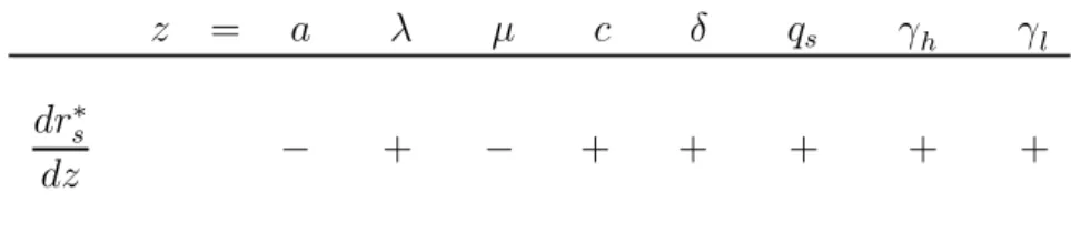
Table 1 summarizes the comparative statics of the equilibrium interest rates on initial loansr∗s, which are derived in Appendix A. The table shows the sign of the derivativedrs∗/dz
obtained by differentiating (10) with respect to each exogenous parameter z. The effects of the various parameters on r∗
s are inversely related to their impact on the profitability of
banks’ lending activity. Other things equal,a andμimpact positively on the profitability of continuation lending; λ affects negatively the profitability of both initial lending (directly) and continuation lending (directly and by reducing the availability of capital in the second period);c has a similar negative effect (with no direct effect on the profitability of continu-ation loans); δ increases the cost of equity funding in both periods; γh and γl increase the burden of capital regulation in the corresponding initial state, as well as in the corresponding continuation state (which will behorl with probabilitiesqs and1−qs,respectively);finally,
qs decreases the profitability of continuation lending because, in the high default state h,
loan losses are higher and the corresponding capital requirementγh may also be higher.
Table 1. Comparative statics of the initial loan rate r∗
s z = a λ μ c δ qs γh γl dr∗ s dz − + − + + + + + values ofkscorresponding to rs∗.
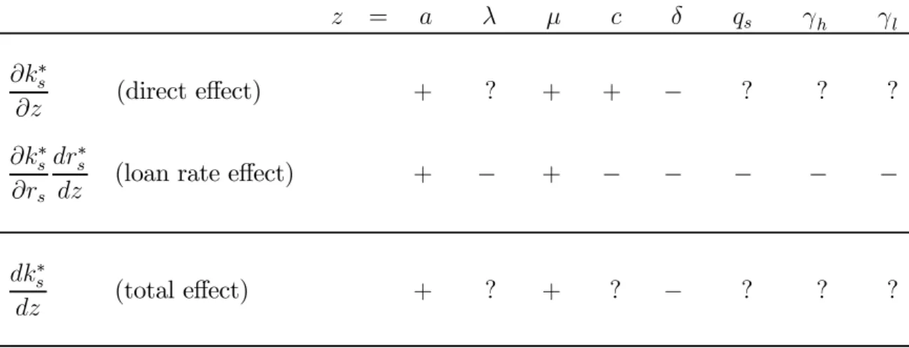
Table 2 summarizes the comparative statics of the equilibrium initial capital k∗
s chosen
by the representative bank in an interior solution–obviously, when the solution is at the corner k∗
s = γs, marginal changes in parameters other than the capital requirement γs do
not changek∗
s.As further explained in Appendix A, the recursive nature of the comparative
statics of the system given by (10) and (11) makes it convenient to decompose the effects of the change in any parameter z into adirect effect (for constantr∗
s) and aloan rate effect
(due to the change inr∗
s): dk∗ s dz = ∂k∗ s ∂z + ∂k∗ s ∂rs dr∗ s dz .
Loan rate effects can be easily determined. Differentiating the first-order condition that characterizes k∗
s in an interior solution gives
∂2v s ∂k2 s ∂k∗ s ∂rs + ∂ 2v s ∂ks∂rs = 0.
The coefficient of ∂k∗
s/∂rs is negative, by the second-order condition that characterizes k∗s
in an interior solution, and the second term is negative (see Appendix A). Hence∂k∗
s/∂rs is
negative, which implies that the signs of loan rate effects are the opposite to those in Table 1. Intuitively, the initial capital ks and the initial loan raters are substitutes in the role of
providing the bank with sufficient capital for its continuation lending (see the definition of
k0s(x) in (2)). In an interior solution, the marginal value of ks is decreasing in ks, and thus
Table 2. Comparative statics of the initial capital k∗
s
(in an interior equilibrium)
z = a λ μ c δ qs γh γl ∂k∗ s ∂z (direct effect) + ? + + − ? ? ? ∂k∗ s ∂rs dr∗ s
dz (loan rate effect) + − + − − − − −
dk∗
s
dz (total effect) + ? + ? − ? ? ?
For the parameters a, μ, and δ, the direct and the loan rate effects point in the same direction, so the total effect can be analytically signed. In essence, higher profitability of continuation lending (captured by a and μ) and lower costs of capital (captured by δ) encourage banks to hold larger capital buffers in order to better self-insure against the default shocks that threaten its continuation lending. For the setup costc, the direct and the loan rate effects have unambiguous but opposite signs, so the total effect is ambiguous. The positive direct effect comes from the fact that, by the definition of k0
s(x) in (2), csubtracts
to the bank’s continuation lending capacity exactly likeks adds to it, without affecting the
profitability of such lending and hence the marginal gains from self-insuring against default shocks. The direct effects on ks of the parameters λ, qs, γh, and γl have ambiguous signs.
Increasing any of these parameters simultaneously reduces the profitability of continuation lending and impairs the expected capital position of the bank when such lending has to be made. The value of holding excess capital in the initial lending period falls, but the prospects of ending up with insufficient capital increase. So the profitability of continuation lending and the need for self-insurance against default shocks move in opposite directions. The resulting ambiguity of the direct effects extends to the total effects.
The details of the analytical expressions suggest that the shape of the distributions of default rates matter for the determination of these effects, which eventually becomes a ques-tion to be elucidated either empirically or by numerically solving the model under realistic parameterizations. Since the goal of the paper is to assess the potential impact of the Basel II capital requirements, which are in the process of being implemented, we resort to the second alternative.
5
Numerical Results
To further explore the forces that affect banks’ initial capital buffers as well as to assess the implications for the dynamics of lending under different regulations, we numerically solve the model in a number of plausible scenarios. Importantly, in all scenarios we assume that the state-contingent probability distributions of the default rate, described by the cdfs Fh(xt)
andFl(xt), conform to the single risk factor model that underlies the capital requirements
associated with the IRB approach of Basel II.21 This means that we assess the implications
of the new capital requirements under the assumption that the supervisor’s model of refer-ence is correct.22 In line with the one-year ahead value-at-risk perspective of Basel II, the
parameterization assumes that each model period corresponds to one calendar year.
5.1
The single risk factor model
Suppose that the project undertaken by entrepreneuri at datet fails ifyit <0, where yit is
a latent random variable defined by
yit =αt+√ρt ut+
p
1−ρt εit,
whereαtis a parameter determined by the state of the economy at datet, utis a single factor
of systematic risk, εit is an idiosyncratic risk factor, and ρt ∈ (0,1) is a state-contingent
21The single factor model is due to Vasicek (2002) and its use as a foundation for the capital requirements of Basel II is due to Gordy (2003).
22Of course, the model could be similarly solved under alternative specifications of the relevant cdfs, but in that case the requirements set under the regulatory formula described below would not have the direct value-at-risk interpretation implied by our parameterization.
parameter that determines the correlation among project failures. It is assumed thatutand
εit areN(0,1) random variables, independently distributed from each other and over time,
as well as, in the case of εit, across projects. Let Φ(·) denote the cdf of a standard normal
random variable. Conditional on the information available at datet,the probability of failure of projectiispt= Pr (yit<0) =Φ(−αt),sinceyit∼N(αt,1),which impliesαt =−Φ−1(pt).
With a continuum of projects, the aggregate failure rate xt is only a function of the
realization of the single risk factorut.Specifically, by the law of large numbers,xt coincides
with the probability of failure of a (representative) projecti conditional on the information available att and the realization of ut:
xt=gt(ut) = Pr ³ −Φ−1(pt) +√ρt ut+ p 1−ρt εit<0|ut ´ =Φ µΦ−1(p t)−√ρt ut √ 1−ρt ¶ .
Using the fact thatut ∼N(0,1),the cumulative distribution function of the aggregate failure
rate can be expressed as
Ft(xt) = Pr (gt(ut)≤xt) = Pr ¡ ut≤g−t1(xt) ¢ =Φ µ√1 −ρt Φ−1(x t)−Φ−1(pt) √ρ t ¶ .
In Basel II the correlation parameter ρt is assumed to be a decreasing function of the state-contingent probability of defaultpt. Hence we postulate the following state-contingent
probability distributions of the default rate
Fs(x) =Φ µ√ 1−ρs Φ−1(x)−Φ−1(ps) √ρ s ¶ , (12)
where, as stipulated by Basel II for corporate loans, the correlation parameterρsis decreasing in the probability of defaultps according to the formula
ρs = 0.12 µ 2−1−e −50ps 1−e−50 ¶ . (13)
In the IRB approach of Basel II, capital must cover the one-year ahead losses due to loan defaults with a probability of 99.9%. Hence the capital requirement in state s is given by
γs=λF−1
s (0.999),where Fs−1(0.999) is the 99.9% quantile of the distribution of the default
rate. Using (12), the Basel II capital requirement becomes
γs=λΦ µΦ−1(p s) +√ρs Φ−1(0.999) √ 1−ρs ¶ , (14)
whereρsis given by (13). This is the formula for corporate exposures of a one-year maturity that appears in Basel Committee on Banking Supervision (2004, paragraph 272).23 It should be noted that Basel II establishes that the expected losses, λps, should be covered with
general loan-loss provisions, while the remaining charge,λ(γs−ps), should be covered with
capital. However, from the perspective of our analysis, provisions are just another form of equity capital, so the distinction between the expected and unexpected components of loan losses is immaterial.
5.2
Benchmark scenarios
Table 3 shows the set of parameter values that define the three benchmark scenarios consid-ered in our numerical analysis. The scenarios differ in the volatility of the state-contingent probabilities of default pl andph. We briefly comment on them here, relegating further
dis-cussion in the light of available data on the US banking sector to Appendix B. Note that because of our normalization of the risk-free rate to zero, all interest rates and rates of return in the parameterization should be interpreted as spreads over the risk-free rate.
Panel A of Table 3 contains the parameters that are common to the three scenarios. The value of the success return a = 0.04 implies that the interest rate of continuation loans is 4%.24 The loss given default (LGD) parameter λ = 0.45 is taken from the Basel II
“foun-dation IRB” formula for unsecured corporate exposures.25 The scale of the second period
projects μ = 1 provides a neutral starting point–fine-tuning this parameter would require some empirical estimation of the growth rate of loan exposures along a typical corporate lending relationship or, alternatively, of the asset growth rate in a representative business
financed by banks. The cost of setting up a lending relationship c = 0.03 is chosen so as yield realistic initial loan rates. The cost of bank capital δ = 0.04 is intended to capture the tax disadvantages of equityfinancing relative to deposit financing. The probabilities of
23The Basel II formula incorporates an adjustment factor that is increasing in the maturity of the exposure, and equals one for a maturity of one year.
24The success return could be higher, as long as the part that can be pledged to the bank without destroying the entrepreneur’s incentives is set at 4%. See Holmström and Tirole (1997) for a discussion of the concept of pledgeable return.
transition to the high default state, ql = 0.20 andqh = 0.64, imply expected durations of 5
years for the low default state and 2.8 years for the high default state, which we calibrate according to the observed behavior of the charge-offratio of FDIC-insured commercial banks in the US during the period 1970-2004.26
Table 3. Parameter values in the benchmark scenarios
A. Common parameters
a μ λ c δ qh ql
0.04 1.00 0.45 0.03 0.04 0.64 0.20
B. Probability of default (PD) scenarios
Benchmark PDs Basel II requirements
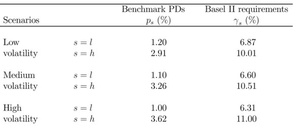
Scenarios ps (%) γs (%) Low s =l 1.20 6.87 volatility s =h 2.91 10.01 Medium s =l 1.10 6.60 volatility s =h 3.26 10.51 High s =l 1.00 6.31 volatility s =h 3.62 11.00
The three PD scenarios are defined so as to keep the expected capital charge under Basel II equal to 8%, which is the capital requirement under Basel I. Appendix B discusses the choice of parameter values in the light of available data on US banks.
Panel B of Table 3 shows our choices for the probabilities of default (PDs) in each state,
pl and ph, and the corresponding Basel II capital requirements, γl and γh, implied by (14).
In each scenario we have chosen the PDs such that the long-run average capital requirement
26Expected durations are computed as q
l+ 2(1−ql)ql+ 3(1−ql)2ql+... = 1/ql = 5 for state l, and (1−qh) + 2qh(1−qh) + 3q2h(1−qh) +...= 1/(1−qh)' 2.8 for stateh. It should be noted that, in line with the empirical findings of Bruche and González-Aguado (2006), in our parameterization credit cycle downturns last longer than typical business cycle downturns.
under Basel II (given the underlying unconditional probabilities of visiting each state) is 8%, as under the risk-insensitive Basel I regulation.27 The idea is to allow for a comparison of the cyclical effects of Basel I and Basel II that is not affected by a change in the long-run average level of the capital requirements. The three scenarios only differ in the magnitude of the cross-state variation in the PDs–and all of them are within a range that can be considered empirically plausible.
It is important to note that we are assuming that the LGD parameterλdoes no depend on the states. Altman et al. (2005), using data on bond defaults,find that LGDs are positively correlated with default rates. In the context of our model, however, cyclical variation in LGDs has a similar effect on banks’ profits and Basel II capital requirements as an increase in the cyclical variation in PDs. Hence, the effects of our conservative assumption could be offset by placing more weight on the results corresponding to the scenarios with more volatile PDs.
5.3
Capital bu
ff
ers and procyclicality
Table 4 shows initial loan rates r∗
s, initial capital ks∗, and the implied capital buffers ∆∗s =
k∗
s−γs,fors=h, l,in each of the scenarios described in Table 3 and under the two regulatory
frameworks that we want to compare: Basel I, with a flat capital requirements of 8%, and Basel II, with the requirements given by (14). As a reference, we also include the results in a laissez-faire environment without capital requirements (γh =γl = 0).
The results show that initial loan rates are always higher in the high default state, reflecting the need to compensate banks for both a higher PD and a lower prospective profitability of continuation lending (since the high default state h is more likely to occur after state h than after state l). These rates are very similar in the two Basel frameworks, confirming previous results from static models predicting that the loan pricing implications of Basel II will be small.28 Basel II slightly increases loan rates in the high default state, and
27The unconditional probabilities of the low and the high default state, denotedφ
landφh,can be obtained by solving the system of equationsqlφl+qhφh=φhandφl+φh= 1,which givesφl= (1−qh)/(1−qh+ql)' 0.64andφh=ql/(1−qh+ql)'0.36.
induces no significant change in loan rates in the low default state. These effects may be explained by the fact that Basel II significantly increases banks’ capital in the high default state, but has a smaller impact on capital in the low default state.
Table 4. Initial loan rates, capital, and capital buffers
(all variables in %)
Basel I Basel II Laissez-faire Scenarios rs∗ k∗s ∆∗s r∗s ks∗ ∆∗s rs∗ k∗s ∆∗s Low s =l 1.2 11.0 3.0 1.2 11.9 5.0 0.7 5.2 5.2 volatility s =h 2.4 11.2 3.2 2.5 12.2 2.2 1.8 5.4 5.4 Medium s =l 1.2 11.0 3.0 1.2 11.7 5.1 0.6 5.1 5.1 volatility s =h 2.7 11.2 3.2 2.8 12.5 1.9 2.1 5.3 5.3 High s =l 1.1 10.9 2.9 1.1 10.7 4.3 0.5 5.0 5.0 volatility s =h 3.0 11.1 3.1 3.1 12.6 1.6 2.3 5.2 5.2
The parameters that define each of the three scenarios and the associated Basel II capital requirements are described in Table 3. The Basel I capital requirement is always 8%.
The results also show that, in order to preserve their future lending capacity, banks hold sizeable capital buffers. Under Basel I, the cyclical variation in PDs has a rather small impact on capital decisions, although excess capital tends to be larger in the high default state (where loan losses can be expected to cause a larger reduction in future lending capacity) than in the low default state.29 Under Basel II the cross-state variability in PDs visibly translates into greater variability of both total capital and capital buffers. Interestingly, the cyclical pattern of the buffers gets reversed, from slightly countercyclical in Basel II to strongly procyclical in Basel II. The main reason for this reversal is that, under Basel II, banks in the low default state l anticipate that if the economy switches to the high default state h the capital requirement will increase from γl to γh. This jump in capital requirements implies
29This is consistent with the existing evidence about the behavior of capital buffers under Basel I– including Ayuso et al. (2004) with Spanish data, Lindquist (2004) with Norwegian data, and Bikker and Metzemakers (2004) with data from 29 OECD countries–and raises doubts about the interpretation that such evidence reflects banks’ myopia.
a reduction in their lending capacity so, to preserve continuation lending, they have an incentive to hold larger precautionary capital buffers than under Basel I, where the capital requirement stays at 8%. Symmetrically, under Basel II, banks in the high default state h
anticipate that if the economy switches to the low default state l the capital requirement will decrease from γh to γl, so they have an incentive to hold smaller capital buffers than
under Basel I. The numerical results for the three scenarios show that thefirst effect (higher buffers in state l) turns out to be more important than the second effect (lower buffers in state h), which implies that the move from Basel I to Basel II will increase the long-run average level of the capital buffers (computed with the unconditional probabilities of visiting each state).30
As for the laissez-faire environment, the results in Table 4 confirm that, under our pa-rameterization, the “economic capital” chosen by banks starting lending relationships is well-below the regulatory capital of any of the two Basel frameworks, but significantly dif-ferent from zero (and very similar across states), which reflects banks’ interest in preserving their valuable lending during the second period.31 The lower initial interest rates in both
states (relative to the Basel frameworks) reflect the savings on the costs of equityfinancing due to the use of less capital in the two lending periods.
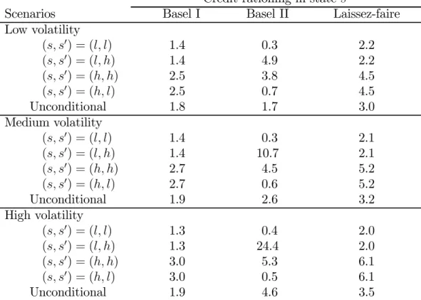
Table 5 compares the cyclical behavior of credit rationing under Basel I and Basel II, as well as in the laissez-faire environment. Lending in any given period is made up of initial loans, whose quantity is always one, and continuation loans, whose quantity varies with the lending capacity of the banks that are unable to issue equity in that period. We denote bycredit rationing the expected percentage of continuation projects that cannot be undertaken because of banks’ insufficient lending capacity. Table 5 shows credit rationing in states0 =l, hwhen it is reached from state s=l, h according to any of the four possible
sequences (s, s0). In our simple model, investment and hence expected gross output (the
returns from the funded investment projects) are linearly related to total credit, given the
30The increase in the medium volatility scenario is of 0.88 percentage points.
31Elizalde and Repullo (2007) discuss the concept of economic capital (and its relationship with the regulatory capital of Basel II) in a model where banks are concerned about the loss of charter values when they become insolvent.
state of the economy, so we can use credit rationing as a summary statistic of aggregate economic activity.
Table 5. Credit rationing
(all variables in %)
Credit rationing in state s0
Scenarios Basel I Basel II Laissez-faire Low volatility (s, s0) = (l, l) 1.4 0.3 2.2 (s, s0) = (l, h) 1.4 4.9 2.2 (s, s0) = (h, h) 2.5 3.8 4.5 (s, s0) = (h, l) 2.5 0.7 4.5 Unconditional 1.8 1.7 3.0 Medium volatility (s, s0) = (l, l) 1.4 0.3 2.1 (s, s0) = (l, h) 1.4 10.7 2.1 (s, s0) = (h, h) 2.7 4.5 5.2 (s, s0) = (h, l) 2.7 0.6 5.2 Unconditional 1.9 2.6 3.2 High volatility (s, s0) = (l, l) 1.3 0.4 2.0 (s, s0) = (l, h) 1.3 24.4 2.0 (s, s0) = (h, h) 3.0 5.3 6.1 (s, s0) = (h, l) 3.0 0.5 6.1 Unconditional 1.9 4.6 3.5
The parameters that define each of the scenarios and the associated Basel II capital requirements are described in Table 3. The Basel I capital requirement is 8%. Credit rationing is the expected percentage of continuation projects that cannot be undertaken because of banks’ insufficient lending capacity. The rows show credit rationing in state s’ when it is reached from state s according to the sequence (s,s’) in thefirst column. Rows labeled ‘unconditional’ show weighted averages based on the unconditional probabilities of each state.
In Basel I (as well as in the laissez-faire environment) credit rationing does not depend on whether the arrival state s0 is a high or a low default state, since the capital requirement is
the previous period, which determine the capital available for continuation lending. The distribution of this random variable depends on the states of the economy in the previous period. This explains why thefigures for Basel I (and the laissez-faire environment) in Table 5 only vary withs in each scenario, and are smaller for s=l than for s=h.
Under Basel II, the impact of bank profits is also present, but the overall effects on credit rationing are dominated by the cross-state variation of the capital requirements, and its endogenous effects on capital buffers. Thus the sequences with (s, s0) = (l, h), and then
those with (s, s0) = (h, h), systematically exhibit the largest credit rationing. Intuitively, in
the low default statel the transition to the high default stateh is less likely than continuing inh after being inh;additionally, in statel the required capital is lower than in stateh. For both reasons, banks hold less capital ins =l than in s = h (see Table 4). But then if the economy ends up ins0 =h, the combination of a lower capitalization in the previous period
and a higher current requirement explains the very sizable contractions in lending capacity shown in Table 5.32 In particular, for the medium volatility scenario, when the economy
goes from the low to the high default state (and despite of the fact that banks hold a capital buffer of 5.1% in the low default state) an average of 10.7% of the continuation projects are rationed, afigure that goes up to 24.4% in the high volatility scenario.
Thus Basel II implies significantly larger cyclical variation in credit rationing (and con-sequently in investment and output) than Basel I. Its incidence on the average level of credit rationing, shown in the rows labeled ‘unconditional’ in Table 5, depends on the volatility of PDs along the cycle. For the medium volatility scenario, the extra cost of Basel II in terms of long-run average credit rationing amounts to about 0.7% of the potential continuation investment.
The behavior of credit rationing in the laissez-faire environment is very much an amplified version of what is observed under Basel I, with levels of rationing that are between 50% and 100% larger. In relation with Basel II, however, the comparison depends on the volatility
32Interestingly, for the sequences withs0 =l (which entail the lowest credit rationing under Basel II), the
effect of bank profits becomes visible again, producing lower rationing in the(l, l)sequence than in the(h, l) sequence.
of PDs along the cycle: except in the low volatility scenario, the laissez-faire exhibits lower cyclicality and, in the high volatility scenario, it even exhibits lower unconditional expected credit rationing.
5.4
Banks’ solvency
We next compare the various regulatory regimes in terms of banks’ solvency. Table 6 reports the probability of failure of the representative bank for each of the scenarios described in Table 3 and each of the possible states of the economy. These probabilities are different for banks making initial loans (that in state s start with capital ks, earn interest rs on
performing loans, and pay the cost c of starting up their lending relationships) and banks making continuation loans (that in statesstart with capitalγs,earn interestaon performing
loans, and do not pay c). Unlike in the results on credit rationing, these probabilities are purely forward-looking (i.e., they do not depend on the state of the economy in the previous period) and hence we only report their conditional-on-s and unconditional values.
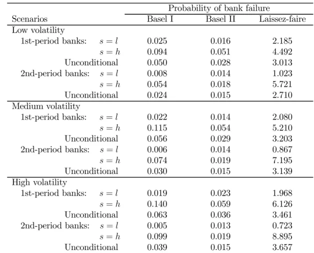
Table 6 shows that the probabilities of bank failure are much more uniform across states under the risk-sensitive capital requirements of Basel II than under the constant 8% capital requirement of Basel I. Conditional on the state of the economy, the link between the level of the requirements and the level of solvency of second period banks is direct (since these banks hold no capital buffers and the net interest income earned on performing loans is the same in both states), so not surprisingly Basel II implies a significant improvement in solvency in the high default state h and a reduction in solvency in the low default state l, with the unconditional effect being clearly positive. For first period banks there are additional effects coming from the endogenous capital buffers and loan interest rates. Our results in Table 4 show that the latter effects are very small, so solvency is inversely related to the total holdings of capital. Hence Basel II increases the solvency of first period banks in state h,
and (in the low and medium volatility scenario) it also increases their solvency in state l, despite imposing lower requirements than the 8% of Basel I. The unconditional effect of Basel II on the solvency offirst period banks is positive in the three scenarios. All in all, Basel II roughly halves the probabilities of bank failure associated with Basel I, and makes the risk
of failure more evenly distributed over time. This suggests that the risk-sensitive capital requirements of Basel II have a payoff in terms of the long-term solvency of the banking system.
Table 6. Banks’ solvency
(all variables in %)
Probability of bank failure
Scenarios Basel I Basel II Laissez-faire Low volatility 1st-period banks: s=l 0.025 0.016 2.185 s=h 0.094 0.051 4.492 Unconditional 0.050 0.028 3.013 2nd-period banks: s=l 0.008 0.014 1.023 s=h 0.054 0.018 5.721 Unconditional 0.024 0.015 2.710 Medium volatility 1st-period banks: s=l 0.022 0.014 2.080 s=h 0.115 0.054 5.210 Unconditional 0.056 0.029 3.203 2nd-period banks: s=l 0.006 0.014 0.867 s=h 0.074 0.019 7.195 Unconditional 0.030 0.015 3.139 High volatility 1st-period banks: s=l 0.019 0.023 1.968 s=h 0.140 0.059 6.126 Unconditional 0.063 0.036 3.461 2nd-period banks: s=l 0.005 0.013 0.723 s=h 0.099 0.019 8.895 Unconditional 0.039 0.015 3.657
The parameters that define each of the scenarios and the associated Basel II capital requirements are described in Table 3. The Basel I capital requirement is 8%. Rows labeled ‘unconditional’ show weighted averages based on the unconditional probabilities of each state.
It is worth noting that the probabilities of bank failure are very small under both regulations–unconditionally, they range between 0.024% and 0.063% under Basel I, and
between 0.015% and 0.036% under Basel II. Interestingly, the combination of capital buffers and net interest income earned on performing loans makes the latter much lower than the 0.1% implied by the 99.9% confidence level of Basel II. This combination also explains the fact that the probabilities of bank failure under the laissez-faire environment are not very high–unconditionally, they range between 2.710% and 3.657%.
6
Policy analysis
Our previous results show that the move from Basel I to Basel II is very likely to imply an increase in the cyclicality of the supply of bank credit. Specifically, we predict a particularly strong reduction in banks’ lending capacity (and a rise in credit rationing) when the economy goes into a recession. The results also suggest that banks’ solvency will be enhanced by the introduction of Basel II.
Consequently, the comparison of Basel I and Basel II in welfare terms is not trivial and will crucially depend on the (structural or reduced-form) imputation of a social cost to bank failures.33 Although the model could be extended to perform such a welfare analysis, the
discussion in this section will be based on the (simpler) argument that it is possible to ameliorate the procyclical impact of Basel II by introducing some small adjustments in the confidence levels set by the regulator. In particular, we consider the possibility of modifying the cyclical profile of confidence levels in such a way that keeps their long-term average at 99.9%–the current level–but lessens the target in those states (or sequences of states) where credit rationing turns out to be the highest under Basel II regulation.
Table 7 shows the results of two specific policy experiments of this kind. Both are performed under the parameterization of the medium volatility scenario described in Table 3. Policy 1 reduces the confidence level in the high default state h to 99.8% and increases the confidence level in the low default state l to η > 99.9% so as to maintain the long-run
33Repullo and Suarez (2004) perform this type of welfare analysis in a static setup where procyclicality is not a concern, but capital requirements imply a deadweigh loss due to the extra cost of equityfinancing.
average at 99.9%. Thusη solves:
η×φl+ 0.998×φh = 0.999,
where φl and φh are, respectively, the unconditional probabilities of the low and the high default state.34 Such a small adjustment causes a relevant change in capital requirements
(from 6.6% to 7.9% forγl and from 10.5% to 9.3% for γh), modifying banks’ optimal buffers (which become less procyclical), and smoothing the cyclicality of credit rationing. As shown in Panel A of Table 7, credit rationing in the sequences(l, h)and(h, h)falls from 10.7% and 4.5%, respectively, to less than 4% in both sequences. Unconditionally, it falls from 2.6% to 1.9%, which is its unconditional value under Basel I. Interestingly, although the probabilities of bank failure in the high default stateh obviously increase, they remain lower than 0.08% in all cells, and their unconditional average only increases from 0.029% to 0.040% for first period banks, and from 0.015% to 0.017% for second period banks.
In Policy 2 we confine the reduced 99.8% confidence level to periods where statehoccurs after state l. The objective is to reduce the credit rationing detected in the second period of sequences with (s, s0) = (l, h). The capital requirement when h occurs after h is left
unchanged, while the confidence level applied to the second period of the sequences (l, l)
and (h, l) is increased so as to to keep the long-run average confidence level at 99.9%. By construction, Policy 2 makes smaller adjustments in the Basel II capital requirements, so it will be less effective than Policy 1 in terms of smoothing credit rationing, but it will also be less significant in terms of its implications for banks’ solvency. The results in Table 7 show that credit rationing in the second period of the(l, h) sequence gets substantially reduced, but not as much as with Policy 1, while the unconditional probabilities of bank failure are almost unchanged relative to those of Basel II.
All in all, our policy experiments show the feasibility of achieving significant gains in terms of credit rationing without major costs in terms of banks’ long-term solvency. This can be achieved with cyclical adjustments that preserve the value-at-risk foundation of the Basel II requirements. The choice between Policy 1 and Policy 2 (or the fine tuning of
34See Footnote 27 for the expressions ofφ
their details) should eventually depend on the trade-off between the gains in terms of a smoother and lower credit rationing, and the losses in terms of less smooth and slightly higher probabilities of bank failure.
Table 7. Procyclicality correction
(all variables in %) A. Credit rationing
Credit rationing in states0
(s, s0) = (l, l) (l, h) (h, h) (h, l) Unconditional Basel I 1.4 1.4 2.7 2.7 1.9 Basel II 0.3 10.7 4.5 0.6 2.6 Policy 1 0.8 3.7 3.6 1.6 1.9 Policy 2 0.5 4.4 4.4 0.6 1.9 B. Banks’ solvency
Probability of failure of 1st-period banks in state s0
(s, s0) = (l, l) (l, h) (h, h) (h, l) Unconditional
Basel I 0.022 0.115 0.115 0.022 0.056
Basel II 0.014 0.054 0.054 0.014 0.029 Policy 1 0.017 0.079 0.079 0.017 0.040 Policy 2 0.019 0.054 0.054 0.019 0.031
Probability of failure of 2nd-period banks in state s0
(s, s0) = (l, l) (l, h) (h, h) (h, l) Unconditional
Basel I 0.006 0.074 0.074 0.006 0.030
Basel II 0.014 0.019 0.019 0.014 0.015 Policy 1 0.007 0.035 0.035 0.007 0.017 Policy 2 0.011 0.035 0.019 0.014 0.016
The parameters and associated Basel II capital requirements are those of the medium volatility scenario described in Table 3. The Basel I capital requirement is 8%. Policy 1 reduces the confidence level of the Basel II formula to 99.8% in stateh and increases it in statel so as to keep the unconditional average at 99.9%. Policy 2 sets the confidence level at 99.8% only when statehoccurs after state l, compensating it when statel occurs so as to keep the unconditional average at 99.9%. Columns labeled ‘unconditional’ show weighted averages based on the unconditional probabilities of each state.