13
Mathematical and Software Engineering, Vol. 3, No. 1 (2017), 13-25 Varεpsilon Ltd, varepsilon.com
Differential Fade Depth with Path Length
Adjustment (DFD-PLA) Method for Computing
the Optimal Path Length of Terrestrial Fixed
Point Line of Sight Microwave Link
Eke Godwin Kelechi, Constance Kalu
*, Akinloye Bolanle Eunice
*Corresponding Author: [email protected]
Department of Electrical/Electronic and Computer Engineering, University of Uyo, Akwa Ibom, Nigeria
Abstract
In this paper, development of Differential Fade Depth with Path Length Adjustment (DFD-PLA) algorithm for calculating the optimal path length for fixed point terrestrial line of sight microwave communication link is presented. The optimal path length for such link is defined as the path length at which the maximum fade depth is equal to the available fade margin the communication system can accommodate at the given set of link parameters. The DFD-PLA algorithm involved iterative adjustment of the path length based on the difference between the effective maximum fade depth and the available fade margin the system can accommodate. Sample 12GHz microwave link is analyzed and the results show that after 28 cycle the algorithm converged when path length, free space path loss and maximum fade depth in the link dropped from their initial to optimal values of 19.9903 km to 5.8726 Km, 140.40 dB to 129.40 dB and 104.04 dB to 30.56 dB respectively.
Keywords: Optimal Path Length; Microwave Link; Fade Margin; Fade Depth; Rain
Fading; Multipath Fading; Differential Fade Depth
1
Introduction
In terrestrial Line of Site (LOS) microwave communication link design, the maximum path length depends, among other things, depends on the Free Space Path (FSP) loss and the maximum fade depth determine from the link, atmospheric and terrain parameters. In practice, mostly rain and multipath fadings are considered and they are taken to be mutually exclusive when determining the maximum fade depth for terrestrial LOS microwave communication links [1, 2]. As such, the maximum fade depth is taken to be rain fading or multipath fading; whichever one is larger.
14
depth. The maximum fade depth determined at the Effective Maximum Path Length is called the Optimal Fade Margin (fmop). At the optimal fade margin, the received signal strength is equal to the receiver sensitivity and the maximum fade depth is equal to the effective fade margin. In essence, the optimal maximum path length is the path length at which the maximum path length determined from the FSP loss (dmfspl) and the maximum path length determined from the computed fade margin (dmcfm) are equal and the received signal strength is equal to the receiver sensitivity.
Accordingly, in this paper, an algorithm is developed for calculating the optimal path length for fixed point terrestrial line of sight microwave communication link. The method involve iterative adjustment of the path length based on the differential fade depth; that is, the difference between the effective maximum fade depth that can be experienced in the link at the specified link percentage availability and the available fade margin the system can accommodate for the given set of link parameters. The iteration ends when the differential fade depth is zero. At this point, effective maximum fade depth and the available fade margin the system can accommodate are equal. The path length at this point is the optimal path length.
2
Methodology
2.1 Determination of The Maximum Transmission Range
Based on Free Space Path Loss and Received Signal
Power
Let be the receiver sensitivity in dBm ; be the received signal power in dBm ; be the specified fade margin in dBm ; be the computed Fade Margin in dBm based on available link equipment and terrain parameters and let dmfspl be the maximum transmission range based on free space path loss. Then
= − (1)
hence = + (2)
Free Space Path Loss Calculation: Based on Friis formula, the expression for computing free space path loss is given as:
LFSP = 32.4 + 20 log(f*1000) + 20 log(d) (3) where LFSP is the free space path loss in dB ; f is the frequency of the emitted signal in GHz and d is the length of the link in km.
Link Budget Calculation: The goal of link budget calculation is to determine the received signal power. Generally, a very simplified version of link budget equation is given as follows:
Received Power = Transmitted Power + Sum of Gains – Sum of Losses (4) PR = PT + (GT + GR ) – (LFSP + LT + LM + LR) (5) where PR is the Received Signal Power (dBm) ; PT is the Transmitter Power Output (dBm); GT is the Transmitter Antenna Gain (dBi) ; GR is the Receiver Antenna Gain (dBi) ; LFSP is the Free Space Path Loss (dB) ; LT is the Losses from Transmitter (cable, connectors etc.) (dB) ; LR is the Losses from Receiver such as cable, connectors etc. losses (dB) and LM is the miscellaneous losses such as polarization misalignment loss, etc. (dB).
15
PR = PT + (GT + GR ) – LFSP (6) Hence,
LFSP = PT + GT + GR - PR (7) Therefore, from Eq. (3), dmfspl (the maximum transmission range based on free space path loss), can be obtained as follows:
d = 10 . !(#∗% ) ' (8 Substituting LFSP from Eq. (7) into Eq.(8) and PR from Eq. (2) into Eq. (8) gives
d = 10() * + ,* + ,- ./0 12 3 . !(#∗% ) 4 (9) With respect to d , the LFSP can be re-calculated as follows;
LFSP = 32.4 + 20 log(f*1000) + 20 log(d ) (10)
Similarly, (effective or computed fade margin the system can accommodate) can be calculated from Eq. (1) and Eq. (6) as follows;
= − = P6 + (G6 + G ) – LFSP − (11)
2.2 Determination of The Maximum Path Length With
Respect to Multipath Fading and Rain Fading
2.2.1 Mathematics of Rain Fade Model
In ITU-R PN.838 recommendations, for frequencies under 40 GHz and path lengths shorter than 60 km, the specific attenuation originating from rainfall is defined as
γ=> in dB/km and modelled using the power-law relationship as follows [5,6,7,8,9]; ? @A = B)CDE3F (12) where CDE is the rainfall rate in mm/h exceeded for GH% of an average year (or stated another way, CDE is the rainfall rate in mm/h for a particular link percentage outage, po). k and α are frequency dependent. Actually, in ITU-R PN.838 recommendation, specific attenuation originating from rainfall is defined separately for horizontal and vertical polarization [10,11,12,13,14]. For the horizontal polarization;
〈? @A〉K = LK)CDE3MN in dB/km (13) For the vertical polarization;
〈? @A〉O = LO)C E3
MP
in dB/km (14)
where:
Kh, αh are frequency dependent coefficients for horizontal polarization rain attenuation . They are given in [15].
Kv, α,v are frequency dependent coefficients for vertical polarization. They are given in [15]
〈? @A〉Kis the rain attenuation per kilometer for horizontal polarization 〈? @A〉Ois the rain attenuation per kilometer for horizontal polarization
GH is the Percentage outage time (or Percentage unavailability time) of the link.
16
GH = (100% − GQ) (15) Rain fade depth, S (dB) is the product of specific rain attenuation, ? @A in dB/km
and the propagation path length, d (km) between the transmitter and the receiver.
S = ? @A' Z (dB) (16) In respect of ITU-R PN.838 [15] recommendation, the following terms can be defined;
S (K)is the rain fade depth (attenuation) for horizontal polarization
S (O)is the rain fade depth (attenuation) for vertical polarization
S [\])is the effective rain fade depth (attenuation) considering both horizontal and vertical polarization.
d is the propagation path length or distance (in km) between the transmitter and the receiver (in this case, d = d )
Hence,
S (K) = 〈γ=> 〉^' d = )K^)R a3
Mb 3 ∗ d
(17)
S (O) = 〈γ=> 〉c' d = )Kc)R a3
Md3 ∗ d
(18)
S [\] = maximum)S (K), S (O)3 (19)
2.2.2 Mathematics of Multipath Fading Model
For quick planning applications, the percentage of time GH that fade depth A j kl mk^ (dB) is exceeded in the average worst month is given as follows [16,17,18].
GH = Kd3.1(1+|εP|)-1.29 ( n.o) 10pqn.nnnor(Ks)q
t/uvwx@ywN'
z{ | % (20)
where:
d is the propagation path length or distance (in km) between the transmitter and the receiver
f is frequency (GHz)
hL is altitude of lower antenna (m)
Amultipath is multipath fade depth (dB)
K is geoklimatic factor and can be obtained from:
K = 10)q}.~qn.nn•€(•‚ƒ)3 (21)
where dN1is the point refractivity gradient
εP is the path inclination, (in mrad). εP is calculated using the following expression [19,20,21]:
…†‡… = (|KwqK‰|)
Š (22)
where:
d is the propagation path length or distance (in km) between the transmitter and the receiver
ℎŒ is the transmitter antenna height
17
Now, multipath Fade Depth, tŽ••Œ\D[ŒK (in dB) is obtain from the expression for GH as follows;
tŽ••Œ\D[ŒK = 10)−0.00089(ℎ“)3 − (10)log p—˜(• .%))ƒ™…šDE@…3 %. ›(œ .•)ž| (23)
The maximum path length due to multipath fading is obtain from the expression for GH as follows:
Let ŠŽ••Œ\D[ŒK be the maximum path length due to multipath fading for any given path
inclination, εP.. Note, ŠŽ••Œ\D[ŒK is the same as d in Eq. (20) and Eq. (22). Then
ŠŽ••Œ\D[ŒK =
Ÿ ¡
¢ £ £ £ £ £ ¤
DE
¢ £ £ £ ¤
¢ £ £ ¤
ƒn
¥ . •›)Ns3' ¦t/uvwx@ywN'z{ §¨
© ª ª «
˜)ƒ™…š@…3 %. ›'(œ .•)
© ª ª ª «
© ª ª ª ª ª « (¬.z)
(24)
2.2.3 The Optimal Path Length and the Differential Fade
Depth Adjustment (DFDA)
In terrestrial LOS microwave link design, rain and multipath fadings are usually considered for determining the maximum fade depth. Fortunately, the mutual relation existing between rain fading and multipath fading rules out the possibility that the link could be affected by both types of attenuation at the same time. As such, the larger of the two types of attenuation determines the value of maximum fade depth in the link. Given that ZŽ is defined as the link maximum fade depth in dB, hence;
ZŽ = Q-® ¯ )tŽ••Œ\D[ŒK, S [\]3 (25)
ZŽ = Q-® ¯ )tŽ••Œ\D[ŒK, S (K), S (O)3 (26) Let Z (K)be the maximum path length due to the rain fade depth (attenuation) for
vertical polarization.
Let Z (O)be the maximum path length due to the rain fade depth (attenuation) for vertical polarization.
Let Z [\]be the maximum path length due to rain fading considering both vertical and horizontal polarization.
Let d a be the Optimal Path Length in km
Let ED be the optimal fade margin in dB Let FSPLa be the optimal free space path loss in dB
Let ZŽ œ• be the maximum path length determined from the computed maximum fade depth (considering both the multipath fading and the rain fading). Then, for any given maximum fade depth ( ZŽ ) in Eq 25 (or Eq 26),
ŠŽ••Œ\D[ŒK , Z (K), Z (O), Š [\] and ZŽ œ•can be computed as follows:
Z (K)° .±/
²b)-> 3³b'
18
Z (O)° .±/
²d)-> 3³d'
(28)
Z [\] = ®´® ¯ )Z (K) , Z (O)3 = ®´® ¯ p µ œ•/
b)=> 3³b' ,
ϥ/
µd)=> 3³d'| (29)
ŠŽ••Œ\D[ŒK =
Ÿ ¡
¢ £ £ £ £ £ ¤
DE
¢ £ £ £ ¤
¢ £ £ ¤
ƒn
¥ ) . •›Ns3 ¦t/uvwx@ywN'z{ §¨
© ª ª «
∗ ˜∗)ƒ™…š@…3 %. ›'(œ .•)
© ª ª ª «
© ª ª ª ª ª « (¬.z)
(30)
ŠŽ œ• = ®´® ¯ )ŠŽ••Œ\D[ŒK , Z (K) , Z (O) 3 (31) The optimal path length (d a ) is obtain when the following conditions are fulfilled;
ŠŽ œ• = d
and ZŽ =
¶ (32)
Hence,
d a = ŠŽ œ• for ŠŽ œ• = d and ZŽ = (33) In this paper, in other to arrive at the optimal path length in Eq 33, the value of the path length, d is adjusted by an adjustment value (dm·¸) and the values of the fade depth ZŽ Q´Z are recomputed. The process is repeated until the optimal path length conditions in Eq 33 are satisfied. The adjustment value dm·¸ can be obtained in several ways among which are;
(i) by using the difference between the fade depth , ZŽand the computed fade margin, . This approach is called the Differential Fade Depth with Path Length Adjustment (DFD-PLA) Method.
(ii) by using the difference between the maximum path length determined from the maximum fade depth, ZŽ œ• and the maximum path length determined from the computed free space path loss, d . This approach is called the Differential Path Length With Path Length Adjustment (DPL-PLA) Method.
However, due to space only the DFD-PLA method is considered in this paper. In the DFD-PLA method, the path length adjustment value for the ith iteration is
defined as dm·¸(l) and can be obtained as follows;
Z[•¹(\)= ( )»¼½¾(l) ™ œ•(œŽº(\) q œ•//(x)(\))34 (34)
19
ED= ZŽ for ZŽ œ• = d and ZŽ = (36) The Optimal Free Space Path Loss (FSPLa ) is given as follows;
FSPLa = 32.4 + 20 log(f*1000) + 20 log(d a ) (37)
2.3 The Differential Fade Depth with Path Length
Adjustment (DFD-PLA) Algorithm
Step 1.1: Input the following link parameters:
f in GHz, PÃ in dBm , GÃ in dBi , G= in dBi , P½ in dBm , in dBm
Step 1.2: Compute the initial maximum transmission range, d (n), which is based on free space path loss in km and the other specified link parameters in Step 1.1 where from Eq. (9):
d (n) = 10(
) * + ,* + ,- ./0 12 3 . !(#∗% ) 4
Step 2: Initialise the iteration counter i, where i = 0
Step 3: Compute the current value of the Free Space Path Loss (in dB),
LFSP(i) from Eq. (10):
LFSP(i) = 32.4 + 20 log(f*1000) + 20 log(d (l))
Step 4: Compute the current value of the Received Power (in dBm) , PR(i) from Eq 6;
PR(i) = PT + (GT + GR ) – LFSP(i)
Step 5: Determine the current value of the effective Fade Margin in dB, (\)
from Eq. (11):
(\) = (\)− = 6 + (Ä6 + Ä ) – LFSP(i) −
Step 6: Compute the current value of the maximum fade depths using the value of
maximum transmission range d = d (l) as follows:
Step 6.1: d = d (l)
Step 6.2: S (K)(\)is current value of the rain fade depth (attenuation) for horizontal polarization from Eq 17;
S (K)(\) = )K^)R a3Mb 3)d (l)3
Step 6.3: S (O)(\)is current value of the rain fade depth (attenuation) for vertical polarization from Eq. (18):
S (O)(\) = )Kc)R a3Md3)d (l)3
Step 6.4: S [\])(\) is the current value of the effective rain fade depth (attenuation) considering both horizontal and vertical polarization,from Eq. (19):
S [\](\)
= maximum )K^)R a3Mb 3)d (l)3, )Kc)R a3Md3)d (l)3'
Step 6.5: K is geoklimatic factor and can be obtained from Eq. (21):
K = 10)q}.~qn.nn•€(•‚ƒ)3
20
…†‡… = (|ℎŒ− ℎŠ •|)
Step 6.7: Amultipath(i) is the current value of the multipath fade depth (in dB), from Eq 23:
tŽ••Œ\D[ŒK(\) = 10(−0.00089ℎ“) − (10)log p—˜ )· DE
Å#Æ> (Ç)3 .%')ƒ™…š@…3 %. ›(œ .•)ž|
Step 7: Compute ZŽ(\), the current value of the link maximum fade depth in dB, which is given in Eq. (26) as:
ZŽ(\) = Q-® ¯ )tŽ••Œ\D[ŒK(\), S (K)(\), S (O)(\)3
Step 8: Compute the excess fade margin ( ÈÉ(\)), where ÈÉ(\) = (\) −
ZŽ(\)
Step 9.1.: If … (\) − ZŽ(\)… > 0.01 then
Step 9.1.1: Compute the path length adjustment from Eq 34:
Z[•¹(\)= p )LFSP(i) + Z( (®) − ZŽ(®))
Ž(\)3|
Step 9.1.2: From Eq. (35):
d (l) = d (l))1 + Z[•¹(\)3
Step 9.1.3: i = i + 1
Step 9.1.4: GOTO Step 3
Step 9.2.1: Else
Step 9.2.2 : Optimal Path Length , d a from Eq. (33):
d a = d (l)
Step 9.2.3: Optimal Fade Margin , fma from Eq. (36):
fma = ZŽ(\)
Step 9.2.4: Optimal Free Space Path Loss , FSPLa from Eq. (37):
FSPLa = FSPL(\)
Step 10: Stop.
3
Results and Discussions
The Differential Fade Depth With Path Length Adjustment (DFD-PLA) algorithm is used to determine the optimal path length for a sample fixed point terrestrial LOS microwave link with the following link parameters: Frequency (f) = 12 GHz; Transmit power (PÃ) = 10dBm; Transmitter Antenna Gain (GÃ) = 35 dBi; Receiver Antenna Gain (G=) = 35 dBi; Fade Margin ( ) =20dB; Receiver Sensitivity (P½) = -80dBm; Rain Zone = N; Point Refractivity Gradient (dN1) = -400; Link Percentage Outage (GH) = 0.01% ; Rain Fade Constants ; BK = 0.01217 , αK = 1.2571 , BO = 0.01129 , αO, = 1.2156; CDE = 95mm/h; ℎŒ = 295 ; and ℎ• = 320m. For each simulation run, the convergence cycle (n) at which the optimal path length is obtained is noted along with other relevant performance parameters.
21
and the rain zone is N, with percentage availability of 99.99% or link percentage Outage (GH) of 0.01% .
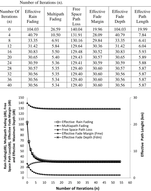
Table 1 Rain Fading, Multipath Fading , Free Space Path Loss , Effective Fade Margin , Effective Maximum Depth and Effective Path Length vs Number of Iterations (n).
Number Of Iterations (n) Effective Rain Fading Multipath Fading Free Space Path Loss Effective Fade Margin Effective Fade Depth Effective Path Length
0 104.03 26.59 140.04 19.96 104.03 19.99
4 40.79 10.50 131.91 28.09 40.79 7.84
8 33.35 6.91 130.16 29.84 33.35 6.41
12 31.42 5.84 129.64 30.36 31.42 6.04
16 30.83 5.50 129.48 30.52 30.83 5.93
20 30.65 5.40 129.43 30.57 30.65 5.89
24 30.59 5.36 129.41 30.59 30.59 5.88
28 30.57 5.35 129.40 30.60 30.57 5.87
32 30.56 5.35 129.40 30.60 30.56 5.87
36 30.56 5.34 129.40 30.60 30.56 5.87
40 30.56 5.34 129.40 30.60 30.56 5.87
Figure 1. Rain Fading(dB), Multipath Fading (dB), Free Space Path Loss(dB) , Effective Fade Margin (dB) , Effective Maximum Depth (dB) and Effective Path Length vs n.
The convergence cycle is 28. That means, as shown in Table 1, Table 2, and Table 3, (as well as, Figure 1, Figure 2, and Figure 3), the DFD-PLA algorithm is iterated for 28 times before the optimal path length is attained.
0 10 20 30 0 10 20 30 40 50 60 70 80 90 100 110 120 130 140 150
0 5 10 15 20 25 30 35 40 45 50 55 60
R ai n F ad in g (d B ), M u lt ip at h F ad in g ( d B ), F re e S p ac e P at h L o ss (d B ), E ff e ct iv e F ad e M ar g in ( d B ) an d E ff e ct iv e M ax im u m D e p th ( d B )
Number of Iterations (n) Effective Rain Fading Multiapath Fading Free Space Path Loss Effective Fade Margin (Fme) Effective Fade Depth (Fdm)
22
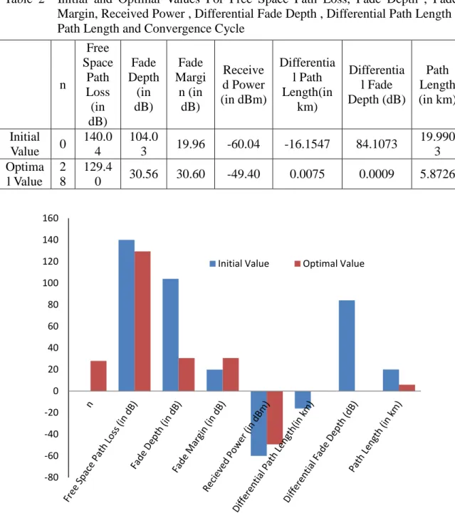
Table 2 Initial and Optimal Values For Free Space Path Loss, Fade Depth , Fade Margin, Received Power , Differential Fade Depth , Differential Path Length , Path Length and Convergence Cycle
n
Free Space
Path Loss (in dB)
Fade Depth
(in dB)
Fade Margi n (in dB)
Receive d Power (in dBm)
Differentia l Path Length(in
km)
Differentia l Fade Depth (dB)
Path Length (in km)
Initial Value 0
140.0 4
104.0
3 19.96 -60.04 -16.1547 84.1073
19.990 3 Optima
l Value 2 8
129.4
0 30.56 30.60 -49.40 0.0075 0.0009 5.8726
Figure 2. Initial and Optimal Values For Free Space Path Loss, Fade Depth , Fade Margin, Received Power , Differential Path Length , Differential Fade Depth, Path Length and Convergence Cycle.
Also, the optimal path length is 5.87 km, the optimal free space path loss is 129.40 dB, the optimal fade margin the system can accommodate is 30.60 dB while the optimal fade depth is 30.56 dB. In essence, at the optimal path length, a maximum fade depth of 30.60 dB can be accommodated by the link. However, the maximum fade depth the rain and multipath fading can present at the optimal path length of 5.87 km is 30.56 dB which is 0. 04 dB short of the optimal fade margin.
It can be recalled from Table 2 and Figure 2 that the initial fade margin specified for the system is 19.60 dB, (actually, 20 dB). At this initial point, in Table 2 and Figure 2, the initial maximum path length is 19.9903 km, the initial free space path loss is 140.40 dB, the initial fade depth is 104.04 dB while the received signal power is -60.04
-80 -60 -40 -20 0 20 40 60 80 100 120 140 160
23
dB. At the optimal point, the free space path loss has reduced by 10.64 dB to a value of 129.40 dB while the received signal power has increased by the same value of 10.64 dB from a value of -60.04 dB to a value of -49.40 dB. From table 1 and Figure 1 , it will be notices that the rain fading is equal to the effective fade depth. Basically, for the given frequency, rain zone and percentage availability, rain fading is greater than the multipath fading and hence, determines the effective fade depth that will be experienced in the link.
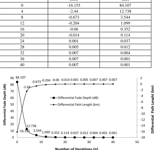
Table 3 Differential Fade Depth and Differential Fade Depth vs Number of Iterations (n)
Number Of Iterations (n) Differential Path Length (km)
Differential Fade Depth (dB)
0 -16.155 84.107
4 -2.44 12.738
8 -0.673 3.544
12 -0.204 1.099
16 -0.06 0.352
20 -0.014 0.114
24 0.001 0.037
28 0.005 0.012
32 0.007 0.004
36 0.007 0.001
40 0.007 0.001
Figure 3. Differential Path Length (DPL) and Differential Fade Depth vs Number of Iterations (n).
4
Conclusion and Recommendations
4.1 Conclusion
In this paper, Differential Fade Depth with Path Length Adjustment (DFD-PLA) algorithm is developed and then used to determine the optimal path length for a sample
84.107
12.738 3.544
1.099 0.352 0.114 0.037 0.012 0.004 0.001 0.001 -16.155
-2.44
-0.673 -0.204 -0.06 -0.014 0.001 0.005 0.007 0.007 0.007
-18 -16 -14 -12 -10 -8 -6 -4 -2 0 2 0 10 20 30 40 50 60 70 80 90
0 10 20 30 40 50
D if fe re n ti al F ad e D e p th ( d B )
Number of Iterations (n) Differential Fade Depth (dB)
Differential Path Length (km)
24
fixed point terrestrial LOS microwave link. The algorithm requires link transmit power and various link equipment and geo-climatic parameters as input. It generates the optimal path length; the optimal free space pathloss; and the optimal fade depth for the microwave link. The DFD-PLA algorithm adjusts the maximum path length based on the fade depth differential, which in this paper is defined as the difference between the maximum fade depth (rain fading or multipath fading, whichever is greater) and the maximum fade margin the system can accommodate. The adjusted maximum path length is used to recalculate the free space path loss, the maximum fade depth and the maximum fade margin the system can accommodate. The procedure is repeated until the maximum path length is found at which the maximum fade depth is equal to the maximum fade margin the system can accommodate.
4.2 Recommendations
In this paper only the Differential Fade Depth with Path Length Adjustment (DFD-PLA) algorithm is considered in which the adjustment to the path length is based on the differential fade depth. It is possible to use the differential path length to determine the optimal path length. As such, further work is required to develop and evaluate the differential path length–based algorithm. Also, it took about 37 iterations before the optimal path length is obtained. More efficient algorithm or adjustment parameter can be used to reduce the number of iterations used to obtain the optimal path length. Accordingly, further work is required to realised the expected improvements.
Furthermore, there is need to evaluate the effect of frequency, link percentage availability and other link parameters on the convergence cycle of the algorithm.
References
[1] Thorvaldsen, P., & Henne, I. (2014) Propagation measurements on a line‐of‐sight over‐water radio link in Norway. Radio Science, 49(7), 531-548.
[2] Angueira, P., & Romo, J. (2012) Microwave Line of Sight Link Engineering. John Wiley & Sons.
[3] Freeman, R. L. (2006) Radio system design for telecommunication (Vol. 98). John Wiley & Sons.
[4] Haykin, S. S., Moher, M., & Koilpillai, D. (2011) Modern wireless
communications. Pearson Education India.
[5] Badron, K., Ismail, A. F., Islam, M. R., Abdullah, K., Din, J., & Tharek, A. R. (2015) A modified rain attenuation prediction model for tropical V‐band satellite
earth link. International Journal of Satellite Communications and
Networking,33(1), 57-67.
[6] Badron, K., Ismail, A. F., Nordin, M. A. W., Isa, F. N. M., & Asnawi, A. (2015) Fade Margin Estimation Technique Using Radar Data for Satellite Link. In Theory
and Applications of Applied Electromagnetics, Springer International Publishing.
(pp. 247-253).
[7] Fenicia, F., Pfister, L., Kavetski, D., Matgen, P., Iffly, J. F., Hoffmann, L., & Uijlenhoet, R. (2012) Microwave links for rainfall estimation in an urban environment: Insights from an experimental setup in Luxembourg-City. Journal of
Hydrology, 464, 69-78.
25
[9] Olsen, R. L., Rogers, D. V., & Hodge, D. B. (1978). The aRb relation in the calculation of rain attenuation. Antennas and Propagation, IEEE Transactions
on, 26(2), 318-329.
[10] Nuroddin, A. C. M., Ismail, A. F., Abdullah, K., Badron, K., Ismail, M., & Hashim, W. (2013). Rain Fade Estimations for the X-Band Satellite Communication Link in
the Tropics. International Journal of Computer and Communication
Engineering, 2(4), 408-412.
[11] Al-Samhi, S. H. A., & Rajput, N. S. (2012) Interference environment between high altitude platform station and fixed wireless access stations. system, 4, 5.
[12] da Silva Mello, L. A. R., Pontes, M. S., De Souza, R. M., & Garcia, N. P. (2007) Prediction of rain attenuation in terrestrial links using full rainfall rate distribution. Electronics Letters, 43(25), 1442-1443.
[13] Ojo, J. S., & Joseph-Ojo, C. I. (2008) An estimate of interference effect on horizontally polarized signal transmission in the tropical locations: a comparison of rain-cell models. Progress In Electromagnetics Research C, 3, 67-79.
[14] Uslu, S., & Tekin, L. (2003) Path loss due to rain fading and precipitation in 26 GHz LMDS systems: consideration of implementation in Turkey. In Microwave
and Telecommunication Technology, 2003. CriMiCo 2003. 13th International Crimean Conference (pp. 68-72). IEEE.
[15] ITU-R838 ITU-R Recommendation p.838-2. Specific Attenuation Model for Rain for Use in Prediction Methods. Interna-tional Telecommunication Union, Geneva (2005).
[16] Asiyo, M. O., & Afullo, T. J. O. (2013) Statistical Estimation of Fade Depth and Outage Probability Due to Multipath Propagation in Southern Africa.Progress In
Electromagnetics Research B, 46, 251-274.
[17] Ghasemi, A., Abedi, A., & Ghasemi, F. (2011) Propagation Engineering in
Wireless Communications. Springer Science & Business Media.
[18] Mohajer, M., Khosravi, R., & Khabiri, M. (2006) Flat Fading Modeling in Fixed Microwave Radio Links Based on ITU-R P. 530-11. In Microwaves, Radar &
Wireless Communications, 2006. MIKON 2006. International Conference on(pp.
423-426). IEEE.
[19] Göktas, P. (2015) Analysis And Implementation Of Prediction Models For The
Design Of Fixed Terrestrial Point-To-Point Systems (Doctoral dissertation, bilkent
university).
[20] Odedina, K. P., & Afullo, T. J. O. (2007) Use of spatial interpolation technique for determination of geoclimatic factor and fade depth calculation in Southern Africa. In AFRICON 2007 (pp. 1-7). IEEE.
[21] Odedina, P. K., & Afullo, T. J. (2008) Estimation of Secondary Radioclimatic Variables and Its Application to Terrestrial LOS Link Design in South Africa, In AFRICON 2008 (pp. 1-6). IEEE.