E
SSAYS ONB
ANKINGC
OMPETITION AND THER
EALE
CONOMYPanit Wattanakoon
A dissertation submitted to the faculty of the University of North Carolina at Chapel Hill in par-tial fulfillment of the requirements for the degree of Doctor of Philosophy in the Department of
Economics.
Chapel Hill 2020
Approved by:
Toan Phan
Gary Biglaiser
Peter Norman
Can Tian
ABSTRACT
PANIT WATTANAKOON: Essays on Banking Competition and the Real Economy. (Under the direction of Toan Phan and Gary Biglaiser)
As big banks grow larger and larger in the past decades, the banking industry become more
and more concentrated. This poses questions on how bank market power affects the real economy.
In this dissertation, I address such economic incidence and try to understand the effects of bank
mark-up on the business cycle and economic growth.
In the first chapter, I simplify Kiyotaki and Moore (1997) into a two-period model, adds bank
market power and study the amplification effects. When borrowers are forced to fire sell their
assets, the asset movement from more to less productive sectors generates adverse feedback toward
the economy. The existence of an imperfect banking market forges the interest spread and raises the
cost of borrowing, making the fireselling agents more constrained and intensifying the recession.
In the second chapter, I study how bank size affects economic growth. The growth model with
a finite number Cournot banks from Cetorelli and Peretto (2012) is simplified into that with two
big and small banks. Big bank with larger equity tends to borrow less, lend more standard loan,
and provide less relationship service than the small one. Nonetheless, I find that the size difference
holding the total credit constant does not deteriorate the growth prospect but rather encourages big
bank to lend and contribute more to economic growth due to its efficiency in providing relationship
ACKNOWLEDGMENTS
I wish to say THANK YOU to many people I met during my Ph.D. study. First and foremost,
I am deeply grateful for my advisor Toan Phan. We spent countless hours on Skype, which he
patiently advised and inspired me. Without his continuous and unfailing support, this dissertation
will not be completed. I want to thank Gary Biglaiser for his encouragement and helpful
sug-gestions. I am thankful to Peter Norman for his questions on various points of my papers. His
contribution helps shape many aspects of the model. I am in debt to Pietro Peretto who provides
invaluable support and piques my interest in this research field. My gratitude is also extended to
Can Tian for her constructive comments and many hours she spends on my papers.
I would like to acknowledge Thammasat University for financial support throughout my five
years in graduate studies. I appreciate administrative arrangements from all staff and directors of
the graduate program in economics. Assistance from all OEADC officers is also recognized.
I thank all the friends I make along this journey. They helped me feel welcome and warm in
my very first and later years here in Chapel Hill. I want to extend my deepest gratitude to my mom
for her understanding and unconditional support, my dad for his inspiration, and my brother for
his devotion to our family. Lastly, I thank my love for her mental support in each and every second
TABLE OF CONTENTS
LIST OF FIGURES . . . vii
1 Banking Competition and the Amplification Mechanism . . . 1
1.1 Introduction . . . 1
1.2 The Model . . . 3
1.2.1 Main model features . . . 4
1.2.2 Equilibrium . . . 8
1.3 The Amplification with Competitive Banks . . . 8
1.3.1 Equilibrium in land market . . . 9
1.3.2 The mechanism . . . 10
1.4 Bank Market Power . . . 13
1.4.1 Equilibrium in land market with the mark up . . . 13
1.4.2 The mechanism with the mark up . . . 14
1.5 Conclusion . . . 17
2 Bank Size and Economic Growth . . . 18
2.1 Introduction . . . 18
2.2 The model . . . 19
2.2.1 Household . . . 21
2.2.2 Firm . . . 21
2.2.3 Capital and Credit . . . 22
2.3 The banking sector’s equilibrium . . . 28
2.4 The equilibrium in capital and output . . . 31
2.5 Conclusion . . . 33
A Appendix . . . 35
A.1 Proof of Proposition 1.3.1 . . . 35
A.2 Proof of Proposition 1.4.1 . . . 37
A.3 Proof of Proposition 1.4.2 . . . 37
A.4 Proof of Proposition 2.3 . . . 38
LIST OF FIGURES
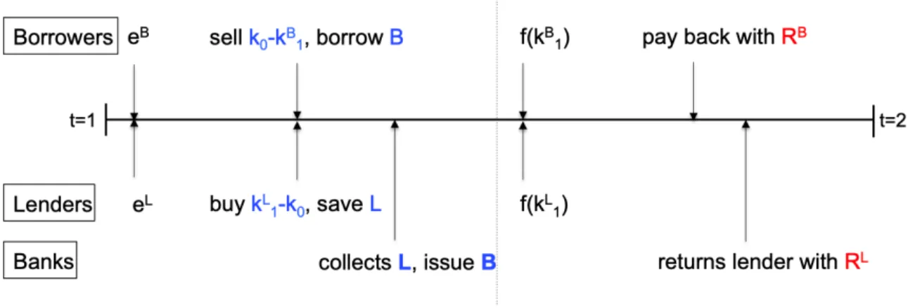
1.1 Timeline . . . 4
1.2 Equilibrium in Land Market . . . 11
1.3 Amplification Mechanism . . . 12
1.4 Monetary Policy and Marginal Cost of Banking . . . 13
1.5 Land Market with Competitive, Oligopolistic, and Monopolistic Banks . . . 15
1.6 Output loss . . . 16
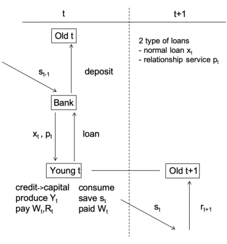
2.1 Timeline . . . 20
2.2 Banks’ optimal choices . . . 29
2.3 Bank’s optimal choices after changes inθandβ . . . 30
2.4 Bank’s optimal choices after a change inδ . . . 31
2.5 Equilibrium inK andm . . . 32
CHAPTER 1
BANKING COMPETITION AND THE AMPLIFICATION MECHANISM
1.1 Introduction
The study on how financial activities affect the real economy is extensively conducted since the
Great Recession1. The deep and persistent slump observed in the real-world business cycle after
the financial crisis attracts more researchers to study the macro-financial linkages. The applications
of micro-founded financing restriction such as costly state verification (Townsend 1979), quantity
rationing (Stiglitz and Weiss 1981), and incomplete contract (Hart and Moore 1994) are prevalent
in the macroeconomic model.
After the onset of the 2008 financial crisis, some banks were out of the business, while some
were merged together. The number of banks in the US fell by 12 percent during 2006-2010 due to
both mergers and bank failures (Wheelock 2011), together with the fact that the higher
concentra-tion ratio of banks in the developed economies has been observed even before the crisis (Mundial
2012). This poses a question on how much bank market power intensifies the economic slump.
This paper simplifies Kiyotaki and Moore (1997) into two-period model, add Monti-Klein
oligopolistic financial intermediaries developed in Klein (1971) and Monti (1972), and compare
the amplification effects. For a competitive banking case, borrowers with a certain degree of
rein-vestment requirement will be forced to sell their input at a price lower than its marginal product.
The relocation from more to less productive producers contracts the economy. For a oligopolistic
case, bank market power contributes to a larger spread between the interest rates. A higher
borrow-ing rate makes constrained agents more in short of resources. It distorts the agents’ behavior and
makes the economy more sensitive to a negative shock. Promoting banking competition alleviates
1See Brunnermeier, Eisenbach, and Sannikov (2013) on a comprehensive review on financial frictions, and
the amplification effect.
The contribution of this paper is to study the collateral constraint in financial friction and market
imperfection in industrial organizations to investigate the oligopolistic banking behavior, examine
the role of market power in the macro-economy, and compare the equilibrium results in different
banking market structure.
Section 1.2 outlines the model on how lenders, borrowers, and financial intermediaries interact.
Section 1.3 is devoted to explaining the amplification mechanism from the lower asset demand
due to consumption and collateral constraints in the economy with perfectly competitive banking
market, while section 1.4 talks about the bank market power as an additional channel to intensified
the recession. Section 1.5 concludes.
Related literature. This paper relates to a few strands of literature. First is the pecuniary exter-nalities from financial friction. Krishnamurthy (2003) studies the amplification mechanism from
collateral constraint due to incomplete contract2 by stripping down the model in Kiyotaki and
Moore (1997) into a finite horizon model. The main characteristics of the paper that distinguish
it apart from other literature such as Bernanke, Gertler, and Gilchrist (1999) is that the aggregate
capital is fixed. The amplification emerges from a lower asset demand of the constrained agent that
dumps down its price and produces the adverse feedback to the economy. Nevertheless, financial
intermediaries were not discussed in this work.
Many later literatures on financial friction include financial intermediaries in their analyses
such as Iacoviello (2015), Sanjani (2014) and Bocola and Lorenzoni (2017) and study their
inter-action with the pecuniary externalities. But little attention is paid on the market power of banks on
the amplification mechanism3.
There is another strand of literature on bank market structure debating on a trade-off between
2When the contract is incomplete (payment in some states of the world is not clearly written), both parties will
renegotiate for their own benefit. Realizing this possibility, the lender will take into account this situation when issuing the initial contract. Ex-ante funding is hardly secured. To rule this out, the collateralized contract is implemented. The repayment is then fully specified in all states of the world.
3For recent work on monopolistic banking, see Andr´es, Arce, and Thomas (2013), and Fujiwara and Teranishi
competition and financial fragility. On the one hand, the competition-instability hypothesis (Allen
and Gale 2004) argues that if all banks are price takers, in order to survive in such an environment,
banks will take excessive risks and the higher probability of default is expected. Diallo (2015)
used data from 145 countries to scrutinize this relationship and found that competition is not good
for a sound banking system. On the other hand, the competition-stability hypothesis argues that
when banks have more market power, a higher interest rate is charged to borrowing companies
(Boyd and De Nicolo 2005). It induces such companies to take more risks to pay all the loans
back. Then a higher possibility that firms will fall and raise the non-performing loans. Anginer,
Demirguc-Kunt, and Zhu (2012) supports this view by empirically discovering that concentration
are prone to greater systemic fragility.
This paper is also related to D´avila and Korinek (2018) which they try to decompose the
pe-cuniary externalities arising from financial friction. In their work, there are distributional and
collateral externalities when agents do not take into account how their actions affect asset prices.
A social planner could internalize those spillovers and achieve constrained efficiency. This paper
talks about these pecuniary externalities and how they are affected by banking market power.
1.2 The Model
Considers a discrete-time economy with a finite horizon for t=1,2. There are 3 agents: a
unit mass of lenders and borrowers, and n number of banks. Borrower and lenders have linear utility function with discount factorsβB and βL both in(0,1), while banks only consume in the
second period. Lenders own half portion of the land: k0 = ¯K/2 and then make decisions on
consumption, one-period deposit, and land purchase. Borrowers also own half of the land, then
decide to consume, borrow, and purchases land for production given the collateral constraint. Both
produce with the same concave production technology f(k1i) = ki1(A −k1i) and are endowed with eL and eB at date 1. The borrower’s endowment can be negative, which implies there is a reinvestment requirement. Figure 2.1 discuss the timeline.
All financial activities regarding borrowing and lending are only facilitated by financial
in-termediaries because we assume that banks are able to collect collateral directly from defaulted
Figure 1.1: Timeline
1.2.1 Main model features
Lenders’ Problem The representative lender optimizes the consumption bundles he wants, the number of lands he purchases, and the amount of deposit he saves. On date 1, lender spends their
expenditure on consumptioncL
1, loan to banksL, and land for the next-date productionq1(kL1−k0).
For the revenue, he obtains his initial endowmenteL. On date 2, he consumes cL2 from his output
f(kL1), and principle plus interestRLL.
max cL
1,cL2,kL1,L
cL1 +βLcL2
subject to
c1L+L+q1(k1L−k0)≤eL (1.2.1)
cL2 ≤f(kL1) +RLL (1.2.2)
cL1 ≥0 (1.2.3)
cL2 ≥0 (1.2.4)
whereRL is the rates of return he gets back after depositing into the banks. q1 is a land price at
date 1. We can find the first-order necessary conditions:
q1 =βLf0(kL1) (1.2.6)
βLRL = 1 (1.2.7)
From equation 1.2.6, the price of land in the first period is determined by its marginal product.
Equation 1.2.7 indicates that the marginal benefit from saving is equal to the marginal cost of this
period consumption forgone.
Borrowers’ Problem The representative borrower faces similar inter-temporal problem to lender but the collateral constraint. On date 1, his revenue comes from his endowment eB, borrowing
made to the bankB limited to the collateral constraint and a portion of capital gain from selling landq1(k0−kB1), while his expenditure is for consumptioncB1. Date 2 budget constraint is similar
to lenders except that borrowers need to repay their debtRBB.
max cB
1,cB2,k1B,B
cB1 +βBcB2
subject to
cB1 ≤eB+q1(k0−k1B) +B (1.2.8)
cB2 +RBB ≤f(k1B) (1.2.9)
RBB ≤θf(kB1) (1.2.10)
cB1 ≥0 (1.2.11)
cB2 ≥0 (1.2.12)
k1B≥0 (1.2.13)
In contrast with the lender’s optimization problem, the borrower’s decision to borrow is restrained
whenθ → 0means no transactions in credit market via bank, whileθ → 1reflects perfect credit market. His debt payment cannot exceed the output he can produce. This is because when the debt
is due, the output is used for repayment instead.
The solution can be derived from setting up Kuhn-Tucker conditions and solving for an optimal
quantity of land demanded as well as borrowing. Given thatf0(0)≥RBq
1 or the marginal product
of land at kB
1 = 0being higher than its land price discounted withRB, the borrower will always
obtain fund from the banks and sacrifice their date-1 consumption since the productivity is higher
than what they need to pay back.
Banks’ Problem We follow the simplified version of banking firm introduced by Klein (1971) and Monti (1972)4. When banks are engaged in deposit and loan, the optimization problem for
a financial intermediary is similar to that of a firm. The profit is derived from the revenue net
cost. Assume that lending and borrowing are only conducted via financial intermediaries due to
their ability to obtain collateral from borrowers. In this section, we consider two different types of
banking structures which are perfectly competitive and oligopolistic markets.
Perfectly competitive banks face the following maximization problem:
max B,L π =R
BB−RLL−C(B)
subject to
B = (1−α)L
Banks obtain funds from lendersL and issue them out to borrower B. The compulsory reserve
α ∈ [0,1], which is controlled by the policymaker, requires banks not to lend all of their deposit. Assume that bank has a linear cost of loan provision: C(B) = γ · B. First-order necessary
conditions are:
RB = R L
1−α +C
0
(B) (1.2.14)
Equation 1.2.14 shows that the marginal benefit from lending to borrower is equal to the marginal
cost of paying interest rate back to depositor and its management cost. For one unit of loan to the
borrower, banks need to find 1−1α unit of deposit to lend out. In the following part, we consider the
oligopolistic financial intermediaries’ problem.
Monti-Klein oligopolistic banks: Suppose that n financial intermediaries with the same cost structure have access to the interbank market. With the market power to set interest rate, each
financial intermediary i faces the following problem:
max Bi,Li
πi =RB(B)Bi−RLLi −C(Bi)
subject to
B = n
X
j=1
Bj =Bi+
X
i6=j Bj
Bi = (1−α)Li
For simplicity, assume that each individual oligopolistic financial intermediary has market power
over the loan market and not on deposit. An individual financial intermediary can control only its
own supply of credit, and choose the optimum amount of loan issued to customers by taking into
account other bankers’ strategies, which affects the borrowing rate of the whole market. Given the
same cost structure, we assume a symmetric equilibrium, in which each setsBi = Bn,Li = Ln. We
can find first-order necessary conditions:
RB+Bi ∂RB
∂B ∂B ∂Bi
∂Bi ∂Li
= R L
1−α +C
0
For equation 1.2.15, the first term of the left-hand side is the marginal benefit of an additional loan
provided, and the second term is the revenue generated from bank market power that it can extract
from credit demand. The right-hand side is similar to a perfect competitive case. We can rearrange
the first-order necessary condition with respect to loan as a price net cost divided by a price (the
Lerner’s index), which is equal to the inverse interest elasticity in equation 1.2.16. Note that the
interest elasticity of borrowing follows: = ∂R∂BB ·
RB
B and when the number of banks approaches
infinity, we have the same first-order necessary conditions:RB = RL
1−α+C
0(B
i)as that in perfectly
competitive case.
RB−RL
1−α +C
0(B
i)
RB =−
1
n (1.2.16)
1.2.2 Equilibrium
Since we have two different banking market structures, we define two different equilibria:
A competitive equilibrium with perfectly competitive banks: is the allocation of quantities and prices as following: {cB
1, cB2, cL1, cL2, π, k1L, kB1, B, L, RB, RL, q1}that satisfy lenders’ optimal
conditions, borrowers’ optimal conditions, collateral constraint, financial intermediaries’ optimal
conditions, market clearing conditionK¯ =k1B+kL1.
A symmetric equilibrium with oligopolistic banks: in which all banks set the same borrow-ing rate RB, and maintain the same quantity of loans and deposits (B
i = Bn and DL1,i = L n for
i= 1,2, . . . , n) is an allocation{cB
1, cB2, cL1, cL2, πi, kL1, kB1}and prices{RL, q1}that solves lenders’,
borrowers’, and financial intermediaries’ maximization problems, and all market clearing
condi-tionK¯ =k1B+kL1.
1.3 The Amplification with Competitive Banks
In this section, we discuss the equilibrium for land market by putting together demand and
supply for land at date 1 and explore the amplification mechanism. The demand and supply are
determined by the borrower’s and lender’s optimal conditions. We will start our analysis on the
1.3.1 Equilibrium in land market
From borrower’s perspective, lenders are land supplier. Optimization condition of lenders
yields the upward sloping supply of land in price at date 1, which takes the form:
Ks(q1) = ¯K−f0−1(
q1
βL) = ¯K+ 1 2
q1
βL −A
(1.3.1)
for βL(A −2 ¯K) < q1 < βLA; otherwise, the solution is at the corner where either lender or
borrower owns all the land. If the land price is too high βL(A −2 ¯K) or twice of its marginal product atkL
1 = ¯K, lenders do not want to buy it and if it is too low βLAor its marginal product
atkL
1 = 0, they will purchase all of it.
For land demand, consider the date-1 optimization problem for borrowers. If date-1
consump-tion and collateral constraints (equaconsump-tion 1.2.11 and 1.2.9) are not binding, we obtain equaconsump-tion 1.3.2
as an unconstrained borrower’s demand for land, which is downward sloping given the concave
production function.
k1Bu=f0−1
q1 βB = 1 2
A− q1 βB
(1.3.2)
When the marginal product of land is higher than its discounted price: f0(0) ≥ RBq1, date-1
consumption constraint binds. The borrower had better sacrifice date-1 consumption to buy more
land for date-2 production and consumption. The constrained borrower’s demand for land can be
expressed as equation 1.3.3.
k1Bc=k0+
eB+B q1
(1.3.3)
If the land price in the first period is high enough and makes date-1 consumption constraint not
binding, the borrower will have more ability to purchase both this period consumption and land
for next-period production. Therefore, the borrower’s demand for land is given by the minimum
of the constrained and unconstrained demands, expressed in equation 1.3.4.
Kd(q1, RB) = min{kBu1 , k
Bc
1 }= min (
1 2
A− q1 βB
, k0+
eB+B q1
)
Consider the effect of price on the constrained demand for land. If the borrowers are forced
to sell their initial land, the higher the land price is, the less land they need to sell (thus demand
more land), the positive relationship between land demand and price is formed, formalized in
proposition 1.3.1, then the constrained borrower’s demand for land is increasing5 inq1, when the
price of land is lower than a thresholdqˆ1 and greater thanq¯1. We will focus on the firesold case.
Proposition 1.3.1 1. If eB ≤ e∗, borrower’s date-1 consumption and collateral constraints are binding.
2. Ifeˆ1 ≤ eB ≤ ˆe2, then we have upward sloping borrower’s demand for land and borrowers
fire sells their land
ProofSee appendix A.1.
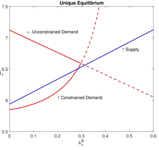
When we combine borrower’s demand and lender’s supply for land to derive the equilibrium
price of landq1. Figure 1.2 shows the numerical result of the unconstrained and constrained
de-mands and supply for land in t=1, given perfectly competitive banking market. When borrowers
are not constrained, the demand for land is downward sloping. Nevertheless, when the borrower
is constrained, the demand for land is instead upward sloping. We then have a kink borrower’s
demand for land. The constrained equilibrium quantity of borrower’s demand for land is lower
than the unconstrained case due to the amplification effect.
1.3.2 The mechanism
The upward-sloping demand for land in equation 1.3.4 is the source of amplification
mecha-nism if borrowers are required to sell their land from proposition 1.3.1. There are two channels
from net worth and collateral constraints. The first one is: When the borrower is required to
rein-vest, his net worth falls and needs fire sell the land to cover that up. The firesold land will be
traded at a lower price than its marginal product; otherwise lender will not purchase it. That will
drive down the land priceq1 and reduce the borrower’s demand for landKd. The second channel is
through the collateral constraint. The falls in net worth and borrower’s demand for land will also
5Dusansky and Koc¸ (2007) provides empirical evidence on upward sloping housing demand to its price since
Figure 1.2: Equilibrium in Land Market
0 0.1 0.2 0.3 0.4 0.5 0.6
kB1 5.5
6 6.5 7 7.5
q1
Unique Equilibrium
Unconstrained Demand
Constrained Demand
Supply
Note: Parameters used for numerical computation are: βL = 0.99, βB = 0.89,K¯ = 1, k0 =
cause a fall in collateral value. Borrowers will be able to borrow less and lower his demand for
land. This amplifies the output contraction further. Figure 1.3 summarizes the idea.
Figure 1.3: Amplification Mechanism
Note: Modified from Kiyotaki and Moore (1997)
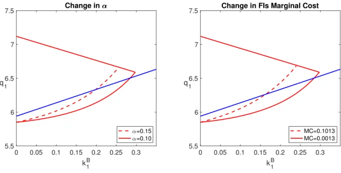
We conduct the comparative statics for the perfectly competitive case to find a tool policymaker
can employ to stimulate the economy. The left panel of figure 1.4 shows that when central bank
lowers the compulsory reserve (α) of the financial intermediaries from 0.15 to 0.1 resulting in a right shift in the borrowers’ land demand, banks will lend more as they have no need to keep
a larger portion of their portfolio in their vault. More credit is provided to borrowers, and the
economy is stimulated.
Better technology in banking can help. This includes a policy tool to reduce costs of screening
and monitoring. Figure 1.4 (right panel) suggests that when financial intermediaries can lower
marginal cost for loan provision, the spread falls and borrowers are able to obtain more credit. The
dashed line of borrower’s land demand shifts to the right. Thus, the economy will not go into that
Figure 1.4: Monetary Policy and Marginal Cost of Banking
0 0.05 0.1 0.15 0.2 0.25 0.3
kB1
5.5 6 6.5 7 7.5
q1
Change in
=0.15 =0.10
0 0.05 0.1 0.15 0.2 0.25 0.3
kB1
5.5 6 6.5 7 7.5
q1
Change in FIs Marginal Cost
MC=0.1013 MC=0.0013
1.4 Bank Market Power
We analyze the amplification in an oligopolistic case. The different market structure for
fi-nancial intermediaries delivers different borrowing rates, which results in a different allocation of
loan.
1.4.1 Equilibrium in land market with the mark up
Supply for land is derived from lenders’ problem which is not directly affected by the change in
the interest rate on borrowers, only indirectly through the change in land demand from borrowers.
Both constrained and unconstrained borrower’s demand for land still follows equation 1.3.4. We
will now focus on how the interest rate on borrowing is related to borrower’s demand for land.
Proposition 1.4.1 If borrower’s net worth and collateral constraints are binding, then Kd is
de-creasing inRB, andRB,P C < RB,O. ProofSee appendix A.2.
From proposition 1.4.1, we find that the borrower’s demand for land is decreasing in the loan
A smaller amount of borrowing means that the borrower cannot afford to buy more land to
pro-duce. As a consequence, borrowers demand less land. Another result we can derive from
propo-sition 1.4.1 is that the equilibrium borrowing rates in the oligopolistic case are larger then that in
the perfectly competitive one. The oligopolistic bank has market power to manipulate the amount
of loan issued to a borrower. In order to maximize profit, the oligopolistic firms can extract some
of the borrowers’ surplus in the credit market by forging higher spread than perfectly competitive
financial intermediaries. They will lend less for higher loan rate and lower borrower’s demand for
land as a result.
Consider the date-1 equilibrium in land market. A higher borrowing interest rate charged by
oligopolistic banks leads to lower equilibrium borrower’s demand for land. Figure 1.5 illustrates
the equilibrium in land market when the credit market is operated by a few banks. The increasing
part of borrower’s demand for land shifts to the left, compared to the perfectly competitive case.
The fall in output is larger when the banking market structure is not perfect. More banks make
equilibrium borrower’s demand for land for both cases higher, and the demand curve approaches
that of perfect competition.
For a monopolistic case, the bank can completely manipulate the total supply of borrowing
and influence the borrower’s demand for land and its price. Since the monopoly lends less and
charges higher a borrowing rate, borrowers have less incentive to borrow to purchase land. When
comparing the equilibrium borrower’s demand for land in perfectly competitive, oligopolistic, and
monopolistic banking markets, the monopolistic-equilibrium borrower’s demand for land is the
smallest than that in other market structures.
1.4.2 The mechanism with the mark up
A higher borrowing rate in the oligopolistic market and its negative relationship with
bor-rower’s demand for land contribute to a lower level of borbor-rower’s demand for landkB,O1 , compared withkB,P C1 . We can conclude that the economy with oligopolistic financial intermediaries is more sensitive to a negative shock than the economy with perfectly competitive financial
intermedi-aries.This is becausekB
1 is decreasing inRB, then given the same shock, largerRB from market
power makes kB
Figure 1.5: Land Market with Competitive, Oligopolistic, and Monopolistic Banks
0 0.05 0.1 0.15 0.2 0.25 0.3 0.35 kB
1
5.5 6 6.5 7 7.5
q
1
PC n=4 n=2 n=1
land, he is more productive than the lender because of the concave production function. The
out-put slump is magnified by an asset movement from more to less productive sectors due to the
constrained borrower and the imperfect credit market. Proposition 1.4.2 formalizes the idea.
Proposition 1.4.2 Given k1B,P C > k1B,O, equilibrium output in perfectly competitive banking market is larger than that in oligopolistic case:yP C
1 > y1O
ProofSee appendix A.3.
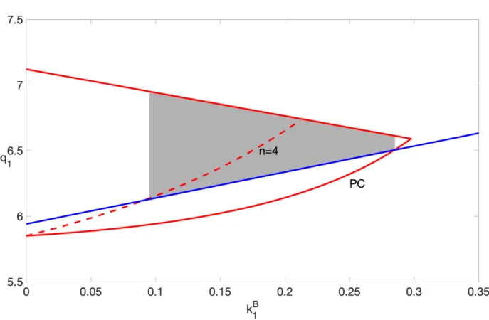
Figure 1.6: Output loss
Note: Parameters used for numerical computation are the same as in figure 1.2.
Figure 1.6 helps visualize proposition 1.4.2. Since the demand curves are derived from the
marginal product of land, the area under the curve, which is the integral of marginal product of
input and input, indicates the amount of output produced by borrowers and lenders. The area
difference between the perfect competition and the oligopoly is shaded and tells us about the output
To avoid a severe contraction in borrower’s demand for land and output when banks have
market power, the central bank can employ a traditional monetary policy to help reduce the cost of
funding and loosen the constrained borrowers’ budget to demand more land as a result.
1.5 Conclusion
The amplification mechanism stems from the lower asset demand that drives down its price and
generates adverse feedback toward the economy. Without financial intermediaries, the
amplifica-tion mechanism is smaller in magnitude. Given the managerial cost of financial intermediaries, the
interest gap is materialized as a result.
With oligopolistic banks, the amplification effect is larger since the borrowing rate is marked
up by the market power. The economy with oligopolistic banks is then more sensitive to a shock
than that with perfectly competitive ones because banks with market power capture the surplus
from other agents. Banking competition should then be encouraged so that the amplification effect
CHAPTER 2
BANK SIZE AND ECONOMIC GROWTH
2.1 Introduction
The banking industry has become more and more concentrated. Federal Deposit Insurance
Corporation (FDIC) reports that there were over 10,000 commercial banks in 1984, but fell to under
5,000 in 2016. After the 2008 economic crisis, McCord and Prescott (2014) found that the biggest
slump of the number of banks is due to the smallest size class, which is those with less than $100
million in assets and that two-thirds of such drop are attributed to the lack of entry. Incidentally, the
US economy expands at a lower rate compared with pre-crisis trend. Many inquiries are conducted
to investigate the relationship between banking market structure and economic growth.
The relationship between banking competition and economic growth is theoretically and
empir-ically ambiguous. Many studies support the view that the more perfectly competitive the banking
market is, the better the credit market functions since the loan rate will be kept at a competitive
rate and support growth (Black and Strahan 2002, Smith 1998, Guzman 2000). On the other hand,
many literature argues that banks with market power have more incentive to screen and monitor
their clients, and issue more loans, fostering economic growth (Petersen and Rajan 1995, Cetorelli
and Gambera 2001, Zarutskie 2006). Nonetheless, some researches suggest that such a
relation-ship is not straightforward and depends on the characteristics of the economy (Deidda and Fattouh
2005, Cetorelli and Peretto 2012).
Given how concentrated the banking market has become, bank size is another prospect we
could model banking competition. Berger and Dick (2007) found that there is an early-mover
advantage in the service industry of banking, using data between 1972 to 2002. Banks that
en-ter markets early enjoy larger market shares. Large banks often secure innovation before fringe
Sanders, and Strahan 2004), and internet banking (Furst, Lang, and Nolle 2002). With better
technology, empirical evidence suggests that bigger banks have lower average cost. Corbae and
D’Erasmo (2014) also modeled dominant and fringe banks’ interaction and investigates how a
change in capital requirement contributes to a change in the banking market structure.
The strategic advantage or disadvantage between large and small banks is not new in the
bank-ing industry. Davila and Walther (2017) discussed how bank size affects bailout policy. In their
model, large banks influence how much taxpayer’s fund is spent since the government will concern
about its size due to a too-big-too-fail story that might create systemic risks.
In Cetorelli and Peretto (2012), Cournot banks provide two types of loans for entrepreneurs:
re-lationship and standard loans. The rere-lationship services guarantee that the credits are successfully
transformed into capital for production, while the standard loans are lent to investment projects
with some degree of failure. They found that when the economy has intrinsic market uncertainty,
less competition leads to more capital accumulation because banks with market power will have
more incentive to provide relationship loans and facilitate entrepreneurs’ investment projects.
Nonetheless, there are different sizes of banks out there in the real economy. The size
dif-ferences might have some implication on economic growth. Thus, Cetorelli and Peretto’s model
could be extended to incorporate banks’ type. This paper aims to study how the banking market
structure with big and small banks affects capital accumulation. We find that the differences in
size foster growth. When the efficient banks becomes larger, they can afford to lend more of both
standard and relationship loans and contribute to higher level of total output.
The paper organizes as following. The next section outlines the model, how households,
en-trepreneurs, and banks behave, and how credit is transformed into capital. Section 3 characterizes
the equilibrium, while section 4 talks about aggregate capital accumulation. Section 5 concludes.
2.2 The model
We study the economy with an infinite horizon. Overlapping generation household and firm’s
setups follows Cetorelli and Peretto (2012), but two banks of banks: big and small. Young
house-hold works, consumes and savesstfor their consumption when old, while firms pay young
Banks are born with an endowmentei: eb =e0+δfor big bank andes =e0−δfor small bank
wheree0 > δ. Banks obtain depositsStfrom young households and lend firmsXt+ 2e0amount of
credit. Apart from a standard credit issuance, they lend a portion of creditpi as relationship loan.
We can think of such a loan as a liquidity insurance against any mishap which can happen in an
investment project. By extending relationship loans, banks incur a costβ, and the provision of this particular type of loan can raise the likelihood of success of the project. A special characteristic
of this loan is that it can be free ridden and will be discussed more in the later subsection. Both
households and firms have no preference for any particular type of bank.
Figure 2.1: Timeline
Timing. Figure 2.1 sums up the timeline of the model. At date t, the young work in firms, save
wages in banks and consumes. Firms receive creditXtfrom banks. If they succeed in transforming
Banks return the deposit plus interest to savers at date t+1.
2.2.1 Household
Consider a unit mass of household who lives for two periods and has no population growth.
The young have no capital endowed, but only one unit of labor, while the old use only the saving
left after work in the period before. Assume that young household supplies labor inelastically
Lt= 1. Household optimizes:
max ct,ct+1,st
U(ct, ct+1) =cαt +c α
t+1, whereα <1 (2.2.1)
subject to
ct=Wt−st ct+1 =strt+1
Let ct and ct+1 be consumption in young and old, respectively. Household decides to save st at
datetand obtain wageWtfrom work. They receive saving plus interest back when old at a rate, rt+1. Solving the above problem yields equation 2.2.2, which is the upward-sloping supply for
saving for banks.
rt+1(St;Wt) =
St
Wt−St
1−αα
(2.2.2)
2.2.2 Firm
There exists a representative firm producing homogenous final goods for the economy. Suppose
its technology satisfies a standard neoclassical production function and Inada conditions.
Yt=F(Kt, Lt) =AKtγL
1−γ
Producer optimizes according to the following demand for capital and labor equations:
Rt=f0(Kt) = γAKγ
−1
t (2.2.4)
Wt=f(Kt) +Ktf0(Kt) = (1−γ)AKtγ (2.2.5)
Prices of both capital and labor depend on their respective marginal products. Firms will hire
young labor with wageWtand obtain credit with loan rate Rtbefore transforming it into capital.
We talk about such technology in the next section.
2.2.3 Capital and Credit
Capital. Entrepreneurs have no endowment and need to borrow from banks in order to invest
it into capital. That is, a unit mass of entrepreneuri∈[0,1]borrows credit from bank and converts it into capital with linear transformation technology:
Kit =ϑiXit (2.2.6)
where ϑi is a random variable, i.i.d. across time and across entrepreneurs, which takes value
one with probabilityθ and zero with probability1−θ andXit is the total credit obtained by an
individual entrepreneur i at time t. Each entrepreneur succeeds with probability less than one, and
if he fails, the expected liquidation value is zero. Assume thatϑi is size invariant for simplicity. Credit. Banks can engage with all borrowers at any optimal scale since they can collect more
savings from the working young if they are short of credit to lend. There are two types of services
banks can provide. The first one is the standard loan that a firm will face uncertainty around their
investment project. The second type of loan is relationship services that is assumed to facilitate
entrepreneurs to succeed in their investment activities.
The relationship loan can be thought of as a contingent liquidity line for entrepreneurs to
bor-row in case of an emergency. A mismatch of inflows and outflows of firms’ financial obligation
with a relationship loan from a bank will successfully invest credit into capital with probability
one. There are some literatures discussing about bank liquidity services and better firms’
perfor-mances (James 1987, James and Wier 1987, Lummer and McConnell 1989, Hoshi, Kashyap, and
Scharfstein 1991, Gatev and Strahan 2006, Shockley and Thakor 1997, and more recently Li and
Ongena 2015)
Free riding feature. An essential feature of the model is the spillover of relationship service
that might incentivize other banks to free ride. If at least one bank offers a relationship loan, all
uncertainty for that entrepreneurs disappears. Other banks will want to issue standard loan to that
particular entrepreneur without incurring relationship costs. There are literature in favor of this
setup. Ongena, Ros¸covan, Song, and Werker (2014) found that bank loan announcement affects
bond spread issued by that particular firm, which is an evidence to support our claim that credit
commitment provides less risky investment perceived by others.
One might argue that banks will want to offer an exclusive relationship contract and hinder a
firm from other banks. But there is no incentive for entrepreneurs to stick with the contract since
there is also another bank out there to borrow, and they can keep borrowing up to their expected
profit without relationship loan. Although banks can threaten firm to withdraw a relationship
contract, firms will find it hard to believe because relationship loans raise the likelihood of success
and the expected profit. Walking away from the contract only hurts banks’ revenue. Evidences in
Detragiache, Garella, and Guiso (2000), Ongena and Smith (2000), Gopalan, Udell, and Yerramilli
(2011), and Presbitero and Zazzaro (2011) suggest that firms borrow from more than one banks to
diversify their sources of fund and/or reduce liquidity risks.
In our model, a bank decides how much they lend to firms either with or without additional
services to accommodate the success of an investment project, taking into account that the other
financial intermediary acts simultaneously on the same population of borrowers. We study how
the interaction between big and small banks about their loan and relationship services affects the
2.2.4 Bank
Suppose that there are two banks: big and small ones. Both banks collect deposits from the
young and issue standard and relationship loans to entrepreneurs. Big and small bank will obtain
endowmenteb =e
0+δandes =e0−δ, respectively1. They both have market power and compete
in Cournot type of setting.
Big Bank Ignoring the time subscript without loss of generality, for Big bank, its expected profit from issuing to an entrepreneuria loan of sizexbi +ebi is2
πib =pbR(xib+ebi)−β
| {z }
issues relationship
+ (1−pb)(1−ps)θR(xbi +ebi)
| {z }
not issue relationship and neither does other
+ (1−pb)(ps)R(xbi +ebi)
| {z }
not issue but the other issues rel
−rxs i
Definepb andpsas the probability that big and small banks offer relationship loans, respectively, since they move simultaneously and employ mixed strategy. βis the cost of a relationship loan.R
is the loan rate from producer optimization problem, whereasris the deposit rate from households’ optimization problem.
The above equation indicates the profit of a small bank from both issuing or not issuing
rela-tionship loan to entrepreneuri. The first term tells the net profit from providing the relationship services. The second term gives the expected profit if none of the relationship loans are given by
any other banks, which is why there is a probability θ attached. The third term is the free-riding profit if at least one bank relates to entrepreneuri. The fourth is the interest paid back to the old.
We can then aggregate over the mass of applicantsi∈[0,1]. Definexb i =
R1 0 x
b
idi,eb =
R1 0 e
b idi.
1We havee
0to make sure that a change inδaffects only the size differenceδnot the total capital of the economy.
2Assume that banks need to issue credits to all entrepreneurs. We rule out a possible profitable deviation in which
Rearrange the equation:
πb =
Z 1
0
pbR(xbi +ebi)−βdi+
Z 1
0
(1−pb)(1−ps)θR(xbi +ebi)di
+
Z 1
0
(1−pb)(ps)R(xbi +ebi)di−
Z 1
0
rxbidi
=n1−(1−θ)(1−pb)(1−ps)oR(xb+eb)−rxb−pbβ
Given how banks give standard and relationship loans to entrepreneurs, we can derive the total
capital from the summation of relationship credit and the expected amount of standard credit.
K =xb,rel+θxb,nor+xs,rel+θxs,nor
We can sum successfully transformed credit by both big and small banks and the expected value
of standard credits by both banks as:
K =n1−(1−θ)(1−pb)(1−ps)oxb+n1−(1−θ)(1−pb)(1−ps)oxs =h1−(1−θ)(1−pb)(1−ps)iX
=mX
where
m= 1−(1−θ)(1−pb)(1−ps) (2.2.7)
Denote X and m as total credit and credit efficiency. This credit efficiency demonstrates how successfully the economy can transform credit to capital. If either type of banks decides to lend
out more relationship loan, the credit efficiency of the whole economy will increase and so does
the total amount of capital. We can rewrite big bank’s optimization problem as in equation 2.2.8.
They choose the amount of credit and relationship services to maximize their profit.
max xb,pb π
Small Bank Apart from being endowed with a smaller amount of endowment, the small bank has a similar objective function. Its expected profit is
max xs,ps π
s =hm·R(mX)−r(X)ixs−psβ (2.2.9)
The equation 2.2.9 gives us the optimization problem of small banks where the first term gives
the net profit of return from both relationship and standard loans. The second is the cost for
relationship services. We will next discuss their decisions on credit issued and relationship services
provided.
Banks’ optimal choices To find an optimal choice of banks in credit issuing, we differentiate equation 2.2.8 with respect to xb, we obtain equation 2.2.10, which implies that the marginal benefit from borrowing including how much it can influence the demand for loans is equal to the
marginal cost from paying back its source of fund.
mR+ (xb+e0+δ)m
∂R
∂xb =r+x b ∂r
∂xb (2.2.10)
The equation 2.2.10 can be rewritten as 2.2.11 and indicates that the spread between loan and
deposit rate depends on the inverse of credit efficiency m. As the economy becomes more and
more efficient in transforming credit into capital, firms will have more productive capital at hand,
and their marginal product in capital will fall, leading to a decrease in loan rate. The second term
in equation 2.2.11 tells us about the market power of big bank: the nominator is for deposits, while
the denominator is for loans.
R r =
1 m
"
1 + xb X
1
r
1 + xb+e0+δ
X+2e0
1
R
#
where the interest elasticities of deposit and loan are expressed as following r = ∂X ∂r r X = α 1−α
W −X W R =
∂X+ 2e0
∂R
R X+ 2e0
=− 1 1−γ
For relationship services, consider big bank’s optimal decision. We differentiate equation 2.2.8
with respect topb yields equation 2.2.12
pb =
0 ifxbhR+m∂R ∂KX
i
∂m ∂pb < β
(0,1) ifxbhR+m∂R ∂KX
i
∂m ∂pb =β
1 ifxbhR+m∂R ∂KX
i
∂m ∂pb > β
(2.2.12)
Forpb ∈(0,1),
β = (xb +eo+δ)
| {z }
credit issued · R |{z} interest rate on relationship loan
· (1 + 1 R
)
| {z }
contribution to capital via contribution to credit efficiency
h
(1−θ)(1−ps)i
| {z }
contribution to aggregate probability
of relationship loan
(2.2.13)
Equation 2.2.12 narrates the big bank’s decision on relationship loan. If the marginal cost of
relationshipβis higher than its marginal benefit, there is no incentive for big bank to engage in re-lationship services, and vice versa. Banks are indifferent and will choose any portion of credits for
relationship loans when the marginal cost and benefit are equal, following equation 2.2.13. More
relationship services will increase the aggregate probability of success in credit transformation and
raise the amount of total capital. Those capital returns will come back to big bank as an interest
For small bank’s optimal choice, we have the following: R r = 1 m "
1 + xXs1
r
1 + xs+eo−δ
X+2eo
1
R
#
(2.2.14)
β = (xs+eo−δ)·R·(1 + 1 R
)h(1−θ)(1−pb)i (2.2.15)
2.3 The banking sector’s equilibrium
Big and small banks obtain a different amount of endowment. We can think of the big bank
as having larger equity than the small one. This difference in size will have an impact on how
they choose their optimal actions against the counterparty. We have the following equations to
characterize the equilibrium for capital and credit efficiency.
1−(1−θ)(1−pb)(1−ps) =
(X1−γ W W−X
1−αα
1 + α(1(W−α−)WX)xXb Aγ(1−(1−γ)xb+eo+δ
X+2eo )
)γ1
(2.3.1)
1−(1−θ)(1−pb)(1−ps) =
(X1−γ W W−X
1−αα
1 + α(1(W−α−)WX)xXs Aγ(1−(1−γ)xs+eo−δ
X+2eo )
)1γ
(2.3.2)
xb+e o+δ (X+ 2eo)1−γ =
β γ2A
n
1−(1−θ)(1−pb)(1−ps)
o1−γ
(1−θ)(1−ps) (2.3.3)
xs+e o−δ (X+ 2eo)1−γ =
β γ2A
n
1−(1−θ)(1−pb)(1−ps)
o1−γ
(1−θ)(1−pb) (2.3.4)
Equations 2.3.1 and 2.3.2 are derived from big and small banks’ optimization problem with
respect to credit called lending curves, while equations 2.3.3 and 2.3.4 are rearranged from big and
small banks’ decisions on relationship services, called relationship curves. The first two equations
indicate the optimal credit each bank will provide given the level of relationship services, while the
other two point out the optimal relationship loan each bank will serve given the amount of credit
issued. Proposition 2.3 dicusses how big and small banks interact each other.
2. big bank lends more than small bank: xb∗+e0+δ > xs
∗
+e0−δ
3. big bank lends less relationship loan than small bank:pb∗ < ps∗ ProofSee appendix A.4.
Proposition 2.3 gives us three results. First, the big bank with larger endowment borrows less
than the small one because it can use an endowment without incurring cost of paying deposit back
to households3. Second, the big bank still lends more than the small one even if they borrow less
since it uses the advantages of its size from endowment to lend more. The third implication is that
the big bank with larger equity can afford in more risk-taking behavior by reducing the number of
relationship services and paying fewer costs.
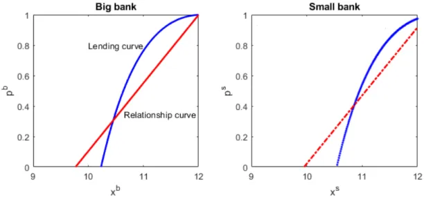
Figure 2.2: Banks’ optimal choices
Note: The figure shows the optimal choice of each bank fixing the other bank’s choice. Parameters used for numerical computation are: e0 = 0.5, δ = 0.1, w = 10, A = 20, β = 3.7, θ = 0.5, γ =
0.5, α = 0.5. LHS fixesxs = 4.8, ps = 0.5, while RHS fixesxb = 5.2, pb = 0.5.
Figure 2.2 illustrates how big and small banks decide their optimal choices in credit and
rela-tionship service. The big bank’s lending curve comes from equation 2.3.1. Its positive relarela-tionship
implies the higher the relationship service, the more borrowing big bank should engage in lending
3During 2015-2019, even if Bank of America has lower level of total equity capital than JP Morgan Chase, the
more and enjoying more profit. The relationship curve from equation 2.3.3 indicates that the more
borrowing, the more relationship service provided to make sure that their lending are successful.
Big bank ends up with a lower level of depositxbcompared with the smaller one.
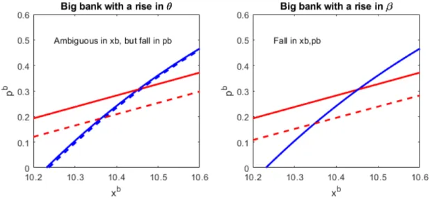
This paper conducts comparative statics of each bank’s optimal choices. Figure 2.3 shows how
a bank responds to the change in the probability of success of the investment project (θ) and the cost of relationship service. A higherθincentivizes bank to lend more as its tendency to obtain the fund back is higher, shifting the lending curve to the right. Still, its marginal benefit of relationship
service is lower so its share of this type of loan falls, shifting the relationship curve to the right.
The right-hand side of figure 2.3 has a rise inβ. A bank decides to lower its relationship service due to its higher cost.
Figure 2.3: Bank’s optimal choices after changes inθandβ
Note: Same set of parameters used in figure 2.2, andθ0 = 0.505,β0 = 3.75
Figure 2.4 illustrates how big and small banks react when there is a change in their size
dif-ference δ. The small bank will borrow more to compensate for a loss in endowment and lend less relationship loan because its stake in investment project or its marginal benefit of relationship
loan is lower. Nonetheless, the small bank choices on xs and ps are ambiguous, depending on
which curve dominates. It borrows less since it has more endowment but lend more relationship
similar to the small bank is drawn.
Figure 2.4: Bank’s optimal choices after a change inδ
Note: Same set of parameters used in figure 2.2, andδ0 = 0.2
2.4 The equilibrium in capital and output
In this section, we study the general equilibrium of aggregate capital (K) and credit efficiency
(m), and conduct comparative statics on how a change in size difference (δ) affects the total output. As we observe in the real world, big banks become larger and larger. Observing how higherδleads to a change in output helps us understand what happens in the economy.
Figure 2.5 shows the equilibrium in capital and credit efficiency. The efficiency curve is solved
numerically from the lending equations 2.3.1 and 2.3.2, pinning down the optimal level of credit
efficiency given capital. A higher level of capital leads to higher credit efficiency. As the economy
has more capital, the marginal product of capital will be lower and thus the interest rate on loan will
fall. To compensate such loss in revenue, banks need to raise relationship loans to make investment
project more successful.
The accumulation curve, on the other hand, is obtained from the relationship equations 2.3.3
and 2.3.4, expressing the optimal capital given credit efficiency. Capital and credit efficiency are
also positively related. As credit efficiency is higher, banks find themselves profitable by lending
minimum value of credit efficiency when both banks decide to lend none of relationship services.
We can study the effect of a change inδ to the equilibrium capital, credit efficiency, and total output. First, consider how a change in δ affects the efficiency curve. Since the efficiency curve reveals the optimalm given capital K, a change in δ does not affect the amount of accumulated capital. In our setup, a rise in endowment of big bank means a fall in endowment of small bank.
The total capital is transformed without depending on the change in the size difference: K = m(xb+xs+ 2e
0). Therefore, there is no change in the efficiency curve after a change inδ.
Figure 2.5: Equilibrium inKandm
Note: Parameters used for numerical computation are: e0 = 5, δ = 0, w = 15, A = 13, β =
10, θ= 0.2, γ = 0.5, α= 0.5.
For the accumulation curve, it gives us an optimal value of capital given credit efficiency. A
rise inδaffects the marginal benefit of relationship service (from equations 2.2.13 and 2.2.15). The big bank will then lend more of relationship loan. Higher relationship services mean the project
has a higher tendency to succeed. Lending more of standard loans will guarantee a better return.
Small bank will react the opposite because its marginal benefit in relationship service falls. The
We then compute how a change inδ affects the total output. Figure 2.6 plots the change in δ
on the horizontal axis and the total output on the vertical axis. Output ends up increasing after an
increase in bank size because big bank dominates by lending more in both standard and relationship
credits. The fixed cost in providing relationship loans plays a major role4. With such cost, a bigger
bank can afford to provide more relationship loans to entrepreneurs without incurring additional
cost per unit of credit. Therefore, a bank with efficient technology can give out more credit line
and liquidity insurance to entrepreneurs and thus help foster economic growth.
Figure 2.6: Output after changes inδ
Note: Same set of parameters used in figure 2.5
2.5 Conclusion
Banks are heterogeneous in their size. This paper studies how big and small banks interact and
how their size differences affects economic growth. We find that big bank with larger equity
bor-rows less from households, lends more loan, and provide less relationship service to entrepreneurs
4However, consider another scenario when the cost of relationship services is linear for example. Its cost is higher
than the small one.
When a big bank gets larger and a small bank gets smaller, the former lends more in both
standard and relationship loans while the latter lends less. Fixed cost in relationship services is the
main reason why big bank engages in more financial activities. Bigger bank lend more credit using
endowment and its marginal benefit of relationship loan is higher, encouraging itself to provide
more relationship services. The credit efficiency is improved and generates more capital, which
implies higher economic growth. If banks are efficient enough, it is willing to lend more and
APPENDIX A
APPENDIX
A.1 Proof of Proposition 1.3.1
1. When the marginal product of land is greater than its cost of buying additional unit of land,
borrower is then willing to purchase land to produce and consume at date 2 instead of date 1. RB
acted as a discount factor between two dates. f0(0)≥RBq
1. We can find the threshold ofeBsuch
thatf0(0) ≥ RBq1 by solvingq1(eB)from demands for land from borrowers and lenders. Plug it
into the above condition and obtaine∗:
e∗ = K¯2+A
21+βL(2−4RB)+βL2RB(−2+3RB)
4βL2RB2 +
AK¯+βL( ¯K−k
0−2 ¯KRB)
βLRB
2. Consider the relationship between land demand and price:
∂kB
1
∂q1
= (k0−k B
1 )/q1
1− θ RBq
1f 0(kB
1)
(A.1.1)
We can either have both nominator and denominator positive:k0−kB1 >0and1−RBθq 1f
0(kB
1 )>
0or negative: k0−k1B <0and1−
θ RBq
1f 0(kB
1)<0, then we have an upward sloping demand for
land ∂kB1
∂q1 >0. First considerk0−k
B
1 :
k0 −kB1 =
−eB−B q1
−eB−B >0⇒k0−k1B >0
eB <−B =−θf(k B
1 )
RB = ˆe2
forced to sell land. Next consider1− θ RBq
1f 0(kB
1 )>0:
1− θ RBq
1
f0(kB1)>0
q1(eB)>
θf0(kB1) RB ⇔eB >eˆ1
Borrower must not sell land too much to drive down its price q1 below the marginal benefit of
borrowing θf0(kB1)
RB . Otherwise, borrowers had better keep land to produce rather than sell it. We
can again solve for a thresholdˆe1andˆe2.
Even though there is a possibility that we can have positive demand for land when both
nomi-nator and denominomi-nator are negative but there will be no feasible range ofeBthat satisfy conditions
of negative nominator and denominator because we would needeB<eˆ
1 andeB >eˆ2.
The relationship between e∗, eˆ1 and ˆe2. We derive e∗ from f0(0) ≥ RBq1(e∗) and ˆe1 from
1− θ RBq
1f 0(kB
1 )>0⇔f0(k0B) < R
B
θ q1(ˆe1)andeˆ2 frome
B <−θf(kB 1)
RB . We can solve and obtain
ˆ
e1 andeˆ2:
ˆ
e1 = 4(βL1RB)2 A2
βL2RB(3RB−4θ)−2βL(RB−2θ)θ−θ2−4AβL(2k
0+ ¯K)θ2
+βLRB(2 ¯KRB+ 2k0θ−3 ¯Kθ)
+ 4βLK¯2k0θ2+βLRB( ¯KRB+ 2k0θ−2 ¯Kθ)
!
ˆ
e2 = 2(RB+2β1LRB−θ)2
"
βLθ −3A2RB+ 3A2βLRB+ 4Ak0RB−4AβLk0RB+ 4βLk02RB
+2AKR¯ B−8AβLKR¯ B−4k
0KR¯ B+ 4βLK¯2RB+ 3A2θ−4Ak0θ−2AKθ¯ + 4k0Kθ¯
−3A4βLk
0(A−2 ¯K)RB(RB+ 2βLRB−θ) + (A((βL−1)RB+θ)−2βL(k0+ ¯K)RB)2 1/2
+2k0
4βLk0(A−2 ¯K)RB(RB+ 2βLRB−θ) + (A((βL−1)RB+θ)−2βL(k0+ ¯K)RB)2 1/2
+2 ¯K4βLk
0(A−2 ¯K)RB(RB+ 2βLRB−θ) + (A((βL−1)RB+θ)−2βL(k0+ ¯K)RB)2
A.2 Proof of Proposition 1.4.1
For the first result, equation 1.3.4 suggests that when loan rate increases, it affects borrower’s
demand for land via binding collateral constraint because borrower will be able to get less loan
and demand less land. The change in loan rate also causes the change in land price because of the
change in land demand. We can think of that change of land price from loan rate as a movement
along the curve when the demand curve shifts.
For the second result, consider bank’s first-order necessary condition in t=1 as following:
RB,P C =C0(B) +RP, and
RB,O −RP +C0(B)
RB,O =−
1 n ⇒ R
B,O−RB,P C RB,O =−
1 n =−
1 n∂R∂BB
RB
B
Apply implicit function theorem on collateral constraint in t=1.
B+ ∂B ∂RBR
B =θf0
(kB1)∂k B
1
RB
1
∂B ∂RB =
θf0(kB
1 )
∂kB 1
∂RB −B
RB
SincekB
1 is decreasing inRB, we have
∂kB 1
∂RB <0and then
∂B
∂RB <0. Therefore,RB,O > RB,P C.
A.3 Proof of Proposition 1.4.2
The overall output produced in t=2 is:
y2 =f(k1B) +f(k
L
1)
=Ak1B−(k1B)2+A( ¯K −kB1)−( ¯K−k1B)2 = ¯KA−K¯ + 2k1B
As long ask1B,P C > kB,O1 , we have a larger output fall in oligopolistic caseyO
A.4 Proof of Proposition 2.3
1. From equations 2.2.10, we have
mR+ (xb+e0+δ)m
∂R
∂xb =r+x b ∂r
∂xb mR−r=
xb
x
r
r −x
b+e
0+δ
X+ 2e0
mR
R
Same for small bank:mR−r =xxsr
r −
xs+e 0−δ
X+2e0
mR
R . We subtract between two equations and
obtain:
xb−xs x ·
r r
= x
b−xs+ 2δ X+ 2e0
mR R ⇔xb−xs = 2δ
X+ 2e0
mR R
1 r Xr −
mR
(X+2e0)R
!
<0
The RHS is negative because the interest elasticity of loanR. Therefore,xb−xs <0. That is, big
bank borrows less than small bank.
2. We can write big and small bank’s FONCs as following:
1−(1−θ)(1−pb)(1−ps) =
(
X1−γWW−X
1−α α
Aγ
1 + 1−ααWW−XxXb (1−(1−γ)xb+eo+δ
X+2eo )
)γ1
1−(1−θ)(1−pb)(1−ps) =
(X1−γ W W−X
1−αα
Aγ
1 + 1−α α
W W−X
xs X
(1−(1−γ)xs+eo−δ
X+2eo )
Use this property BA = DC = BA++CD = BA−−CD ⇒.
2 + 1−ααWW−X 1 +γ =
xb−xs
X
1−α α
W W−X −Aγ(1−γ)(xbX−+2xs+2e δ)
0
2 + 1−ααWW−X 1 +γ
| {z }
+
=
−
z }| {
xb −xs
X
+
z }| {
1−α
α
W W −X
−(1−γ)Aγ
X+ 2e0
| {z }
−
(xb−xs+ 2δ)
| {z }
must be+
We know from proposition 2.3 thatxb −xs < 0. Then,xb −xs+ 2δ must be positive so that the
LHS is positive. Therefore,(xb+e
0+δ)−(xs+e0−δ)is positive. Big bank lends more credit.
3. From equation 2.2.13 and 2.2.15, we can write
xb+e o+δ (X+ 2eo)1−γ
= β γ2A
n
1−(1−θ)(1−pb)(1−ps)o1−γ (1−θ)(1−ps)
xs+e o−δ (X+ 2eo)1−γ
= β γ2A
n
1−(1−θ)(1−pb)(1−ps)o1−γ (1−θ)(1−pb)
⇒ps−pb = (1−pb)(1−ps)(1−θ)γ
2A
βm1−γ
| {z }
+
"
xb−xs+ 2δ (X+ 2e0)1−γ
#
We know from 2.3 thatxb −xs+ 2δ > 0and total creditX+ 2e
0 > 0. Therefore,ps−pb > 0.
REFERENCES
Akhavein, J., W. S. Frame, and L. J. White (2005). The diffusion of financial innovations: An examination of the adoption of small business credit scoring by large banking organizations. The Journal of Business 78(2), 577–596.
Allen, F. and D. Gale (2004). Competition and financial stability. Journal of Money, Credit and Banking, 453–480.
Andr´es, J., O. Arce, and C. Thomas (2013). Banking competition, collateral constraints, and optimal monetary policy. Journal of Money, Credit and Banking 45(s2), 87–125.
Anginer, D., A. Demirguc-Kunt, and M. Zhu (2012). How does bank competition affect systemic stability? the world bank. Development Research Group, Finance and Private Sector Develop-ment Team. Policy Research Working Paper 5981.
Berger, A. N. and A. A. Dick (2007, Jun). Entry into banking markets and the early-mover advan-tage. Journal of Money, Credit and Banking 39(4), 775–807.
Bernanke, B. S., M. Gertler, and S. Gilchrist (1999). The financial accelerator in a quantitative business cycle framework. Handbook of macroeconomics 1, 1341–1393.
Black, S. and P. E. Strahan (2002). Entrepreneurship and bank credit availability. Journal of Finance 57(6), 2807–2833.
Bocola, L. and G. Lorenzoni (2017). Financial crises and lending of last resort in open economies. Technical report, National Bureau of Economic Research.
Boyd, J. H. and G. De Nicolo (2005). The theory of bank risk taking and competition revisited. The Journal of finance 60(3), 1329–1343.
Brunnermeier, M. K., T. M. Eisenbach, and Y. Sannikov (2013). Macroeconomics with financial frictions: A survey. In Advances in Economics and Econometrics: Volume 2, Applied Eco-nomics: Tenth World Congress, Volume 50, pp. 3. Cambridge University Press.
Cetorelli, N. and M. Gambera (2001, Apr). Banking market structure, financial dependence and growth: International evidence from industry data. The Journal of Finance 56(2), 617–648.
Cetorelli, N. and P. F. Peretto (2012). Credit quantity and credit quality: Bank competition and capital accumulation. Journal of Economic Theory 147(3), 967 – 998.
Claessens, S. and M. A. Kose (2017). Macroeconomic implications of financial imperfections: a survey. The World Bank.
Corbae, D. and P. D’Erasmo (2014). Capital requirements in a quantitative model of banking industry dynamics.